
Abstract
The array of periodic scatterers is known as sonic crystal at present and sonic crystal is the most cost-effective solution for a “noise barrier” because of its acoustic attenuation due to size, geometry, and periodic arrangement of scatterers. The simulation methods to estimate acoustic attenuation and the Bragg band of the periodic scatterers have been demonstrated in this paper. First, the periodic cylindrical and C-shaped scatterers have been studied along with the effect of thermo-viscous losses to establish the simulation method. Next, in the laboratory environment, the measurements have been carried out for periodic cylindrical and C-shaped scatterers and the experimental results are in good agreement with simulation results.
Introduction
Periodic scatterers can attenuate sound at certain frequency ranges due to Bragg diffraction and those frequency band are known as Bragg band. The acoustic performance of periodic scatterers is measured by the Insertion Loss (IL) and expressed in decibels (dB).1,2 The said parameters have been evaluated by researchers, majorly in three ways. The first one is an analytical technique, second one is a numerical simulation, and the third one is experimental measurements. Numerical simulation is having advantages over other methods to evaluate when the design of the scatterers is geometrically complex.
At first, the array of cylinders have been presented as a sound sculpture. 3 The sound attenuation via periodic rigid cylindrical scatterers has received significant attention from various researchers due to its simple geometry. However, extremely large size of cylindrical scatterers is required to attenuate noise at a low-frequency regime. Therefore, substantial research has been conducted to enhance the potential of periodic scatterers in controlling the sound in the low-frequency regime.4–6
In general, low-frequency attenuation needs extremely large size scatterers. So, researchers explored the resonant and multi resonant scatterers to attain so. Apart from the Bragg band, a narrow attenuation in a lower frequency regime can be achieved due to the resonance of the scatterers.7,8 Substantial research has been conducted to enhance the potential of periodic scatterers in controlling low-frequency noise. The locally resonant scatterers have received significant attention in the last decade as they have the potential to attenuate sound in a low-frequency regime. Later, multi-resonant periodic scatterers have evolved to attain multiple band gaps in the lower-frequency regime.9–11 Peiró-Torres et al. 12 numerically calculated and experimentally measured the acoustic performance of sonic crystal made of periodic resonant scatterers. They reported two bands of sound attenuation called as resonance bandgap and the Bragg bandgap, where, the resonance band is observed in the lower frequency range before the Bragg band. Redondo et al. 13 increased the performance of sound attenuation of sonic crystal noise barrier using different configurations and orientations of periodic scatterers made of Helmholtz resonators.
In recent years, periodic scatterers based noise barriers are getting a lot of attention over conventional noise barriers in many practical applications. Recent developments in periodic scatterers for attenuating road traffic noise were discussed by Fredianelli et al. 14 A detailed review of periodic scatterers and their applications such as noise barrier, acoustic filter, acoustic imaging, sound cloaking and maze, and waveguiding were discussed by researchers.15–21 Iannace et al. 21 investigated the effect of various geometries and configurations on sound attenuation of meta-material noise barrier and the acoustic barrier was made of periodic cylindrical scatterers.
Romero-Garcet al. 22 designed absorbent resonating scatterers, which can be used as a wideband acoustic filter. The scatterers were made of cylindrical rigid walls having resonant cavities and shielded with absorbent materials. The proposed structure produced high attenuation and exhibits additional esthetic and constructive characteristics compared to conventional noise barriers. Koussa et al. 23 proposed a low-height noise barrier based on resonance and absorption. The insertion and reflection coefficients were studied and compared with the conventional barrier, where, a significant enhancement has been achieved.
As the present research as a whole aims to design new scatterers, the simulation has been found suitable, followed by experimental measurements to authenticate the observations made from the simulation.
Following the present section of introduction, the underlying theory and design of the scatterers have been discussed in sections 2 and 3, respectively. The simulation technique and the results obtained from simulations have been discussed in sections 4 and 5, respectively. In section 6, the effect of thermo-viscous losses in calculated IL has been presented. The detailed sample preparation, experimentation, and measured IL have been presented in section 7, followed by conclusions.
Underlying theory
The frequency domain simulations have been conducted to calculate the IL of periodic scatterers. The simulations have been carried out in COMSOL© pressure acoustic module, by solving lossless wave equation with desired boundary conditions, which can be stated as 24 :

where, ∇ is the Laplacian operator and k is the wavenumber and

The f is frequency in Hz, and c0 is the speed of sound at ambient temperature. The p is the total sound pressure, which can be written as summation of incident sound pressure (pin) and scattered sound pressure (ps), that is,

The acoustically rigid scatterers are modeled using Dirichlet boundary condition and can be stated as:

Here, the ‘
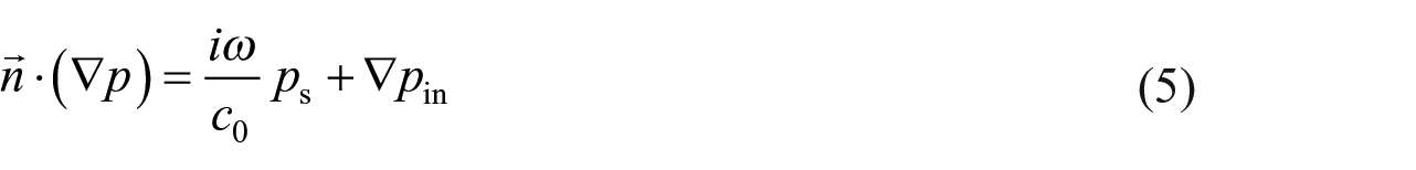
The outlet boundary needs to be acoustically non-reflective. The characteristic acoustic impedance (z0 = ρc0) is to simulate a non-reflective boundary applicable to the plane wave only. So, the perfectly matching layer (PML) is opted. The width of PML is an important parameter in simulation and in present research it is taken as λ/4 of the lowest frequency of interest. The PML is an additional acoustic domain and is connected with the simulation domain.
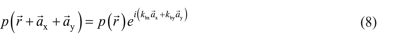
In the present research, the scatterers are infinitely periodic in the direction perpendicular with respect to the propagation of the sound wave. So, the Floquet periodic boundary condition has been applied on the walls of the simulation domain to mimic the infinitely periodic arrangement of scatterers in the normal direction to the corresponding surface and can be stated as:

where, the p
dst
or p
src
is the sound pressure and the subscripts “dst” and “src” are referring to two walls which are bounded to imitate the periodic domain. The
Periodic scatterers
To establish the simulation, the periodic scatterers have been taken from the literature for study. 25 The scatterers are made of periodic cylindrical and C-shaped scatterers. At first, cylindrical scatterers have been simulated. The outer diameter of the scatterer is denoted as d and the distance between two consecutive scatterers in both X and Y directions have been taken the same and denoted as d1. In the given simulation, the d is 400 mm and d1 is 200 mm. The scatterers are organized in a square lattice structure and the lattice constant is denoted as a, which is 600 mm.
Next, periodic C-shaped scatterers have been examined. The C-shaped scatterer is a cylindrical shell having a vertical slit. 25 The diameter (d) of the shell is 400 mm, the distance between two consecutive scatterers (d1) in both X and Y directions is 200 mm, the shell thickness (t) is 10 mm, and the opening of the slit width (w) is taken as 100 mm. The scatterers are organized in a square lattice structure and the lattice constant (a) is taken as 600 mm.
Simulation
Calculation of band structure
The simulation domains with the Cartesian coordinate system have been shown in Figure 1. The 2D unit cell for cylindrical and C-shaped scatterers has been shown in the same figure used to calculate the band structure. For unit cells, a is taken as 600 mm.

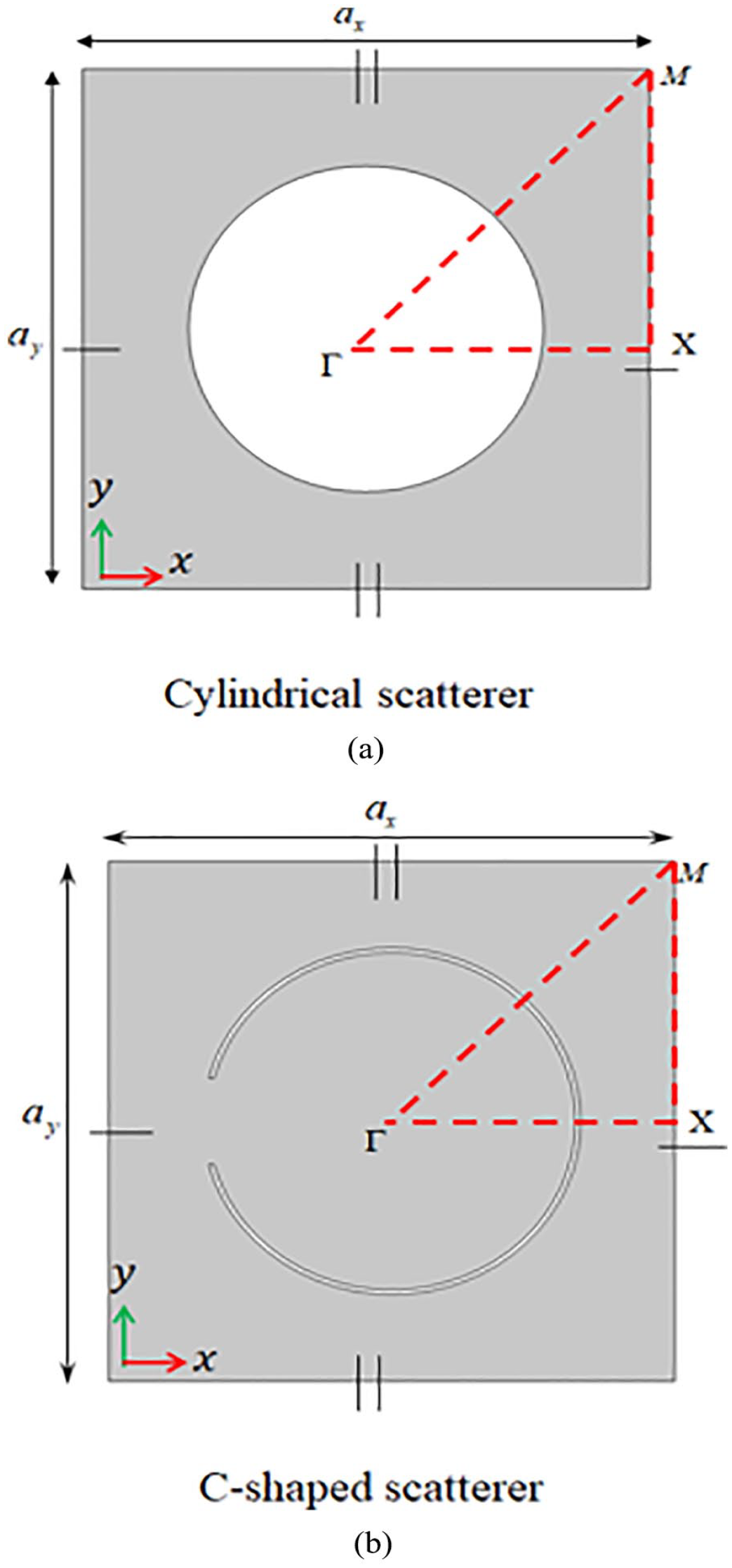
Simulation domain for band structure calculation; (a) cylindrical scatterer, and (b) C-shaped scatterer.
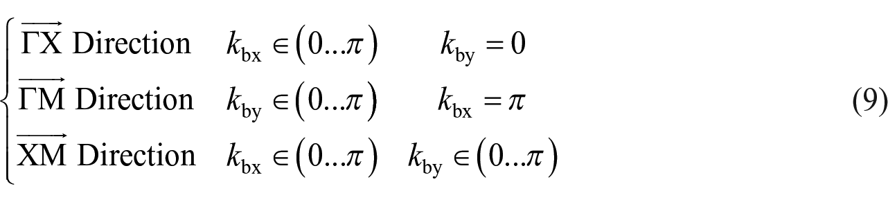
The band structure has been calculated in the
where the
Calculation of insertion loss
Then, five rows of periodic cylindrical scatterers have been studied, where, the scatterers are infinitely periodic in the Y-direction, and is shown in Figure 2(a). The incident wave has been applied to the inlet of the simulation domain. Similarly, five rows of C-shaped scatterers have been shown in Figure 2(b). The C-shaped scatterer is a cylindrical shell having a vertical slit and acts as a Helmholtz resonator. In the simulation, the incident sound wave is in the positive X-direction and the slit openings of the periodic C-shaped scatterers are facing toward it.
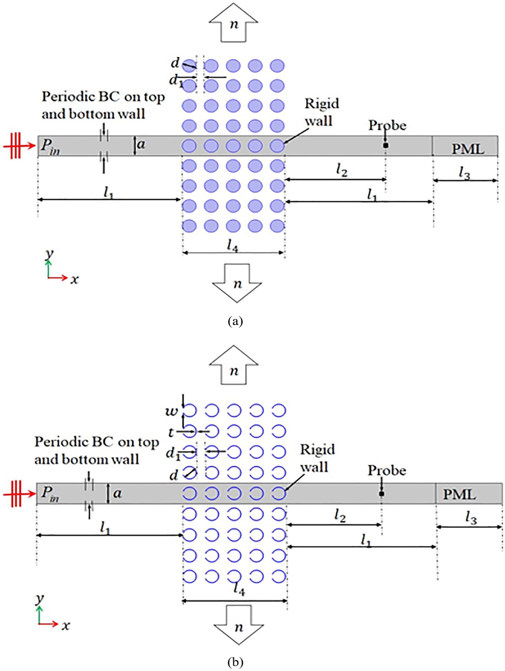
Simulation domain for calculating IL of periodic; (a) cylindrical scatterers (5 rows), and (b) C-shaped scatterers (58 rows).
The applied boundary conditions for calculating IL are:
(a) The plane wave radiation boundary condition is applied with pressure amplitude pin = 1.0 Pa (peak to peak) or of root mean square (RMS) value 0.707 Pa. Then
(b) The PML of length (l3) is applied on right side of the wall to simulate the acoustically non-reflecting boundary condition.
(c) The top and bottom walls are applied with Floquet periodic boundary conditions to simulate the infinite periodic arrangement in the Y-direction.
(d) The walls of the scatterers have been made acoustically rigid.
(e) The frequency domain simulations are carried out from lower frequency to higher frequency with a given frequency resolution.
The IL has been calculated with help of a sound pressure probe. The sound pressure without scatterers denoted as SPL NS is subtracted by sound pressure with scatterers denoted as SPL W S . As the lossless wave equation has been solved, the sound pressure inside the domain, without scatterers, is observed at 90.9 dB. So, it can be written as:


The dimension of l1 is taken with an assumption of lambda (λ) corresponding to 200 Hz for achieving maximum accuracy in the simulation. The l2 is the distance between the end of scatterers to the location of the probe, where the probe is placed in the near-field. The perfectly matched layer (PML) having a thickness (l3) is attached to the right side of the simulation domain to reduce the reflections from the outlet. The (l3) is taken around one-sixth of the lambda (λ), which is around 0.3 m. The total width of the periodic scatterers is denoted by (l4).
The length of the simulation domain before and after the periodic scatterers have been denoted as l1 and l1, and taken as 1 m. A point sound pressure probe is placed l2 distance (X-direction) from the scatterers and middle of the simulation domain in Y-direction, and l2 is taken as 0.2 m. Thickness (l3) of a perfectly matched layer is attached to the right side of the simulation domain to reduce the reflections and the l3 is taken as 0.3 m. The total length of array of the scatterers is defined as l4.
The free triangular elements are used for meshing the simulation domain. The triangular element meshes are generated with a maximum element size of;

where, Emax is the maximum element size, c0 is speed of sound in air, c0 = 344 ms−1 and fm is the maximum frequency of interest. In meshing, the minimum size of elements is 1e−6 m, the maximum element growth rate is 1.1, the curvature factor is 0.1 and resolution of narrow region is 1. In the given simulation, the fm is 450 Hz. The frequency domain simulations have been carried out from 20 Hz to 450 Hz with a frequency resolution of 5 Hz. Figure 3 shows the 2D meshing of five rows of periodic scatterers.
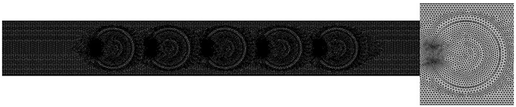
Meshing of the simulation domain used for calculating IL (C-shaped scatterer with a slit is shown on right side).
Results and discussion
For illustration purposes, few notations have been formulated to describe the IL. The amplitudes of the lower and upper boundaries of the first Bragg band are around 0 dB and are denoted with
Apart from the Bragg band, there is a sudden peak in IL toward infinity (very high amplitude) for the resonant scatterers. This is denoted by fn∞.
Cylindrical scatterers
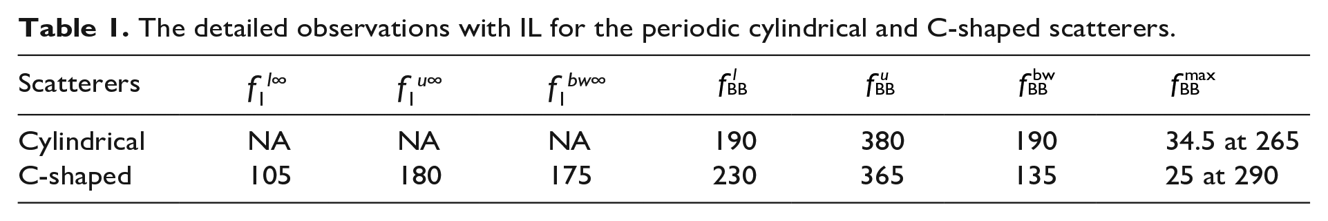
The calculated band structure and IL of five rows of periodic cylindrical scatterers have been shown in Figure 4. The detailed observations with IL for the periodic cylindrical scatterers have been tabulated in Table 1. The band gap has been observed between frequencies of 190 to 380 Hz, which is due to its Bragg diffraction. From IL, the
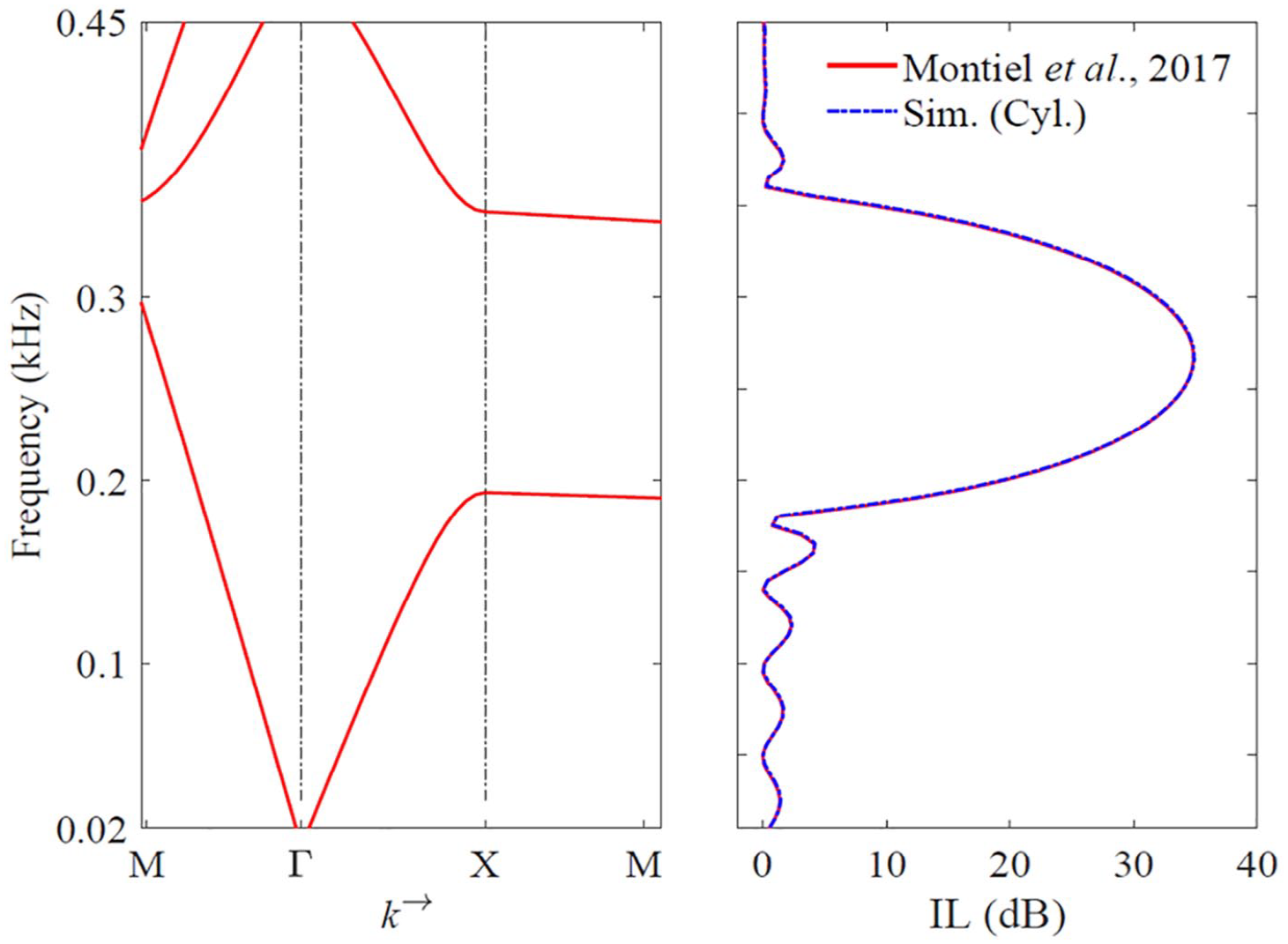
Calculated band structure and IL of cylindrical scatterers.
The detailed observations with IL for the periodic cylindrical and C-shaped scatterers.
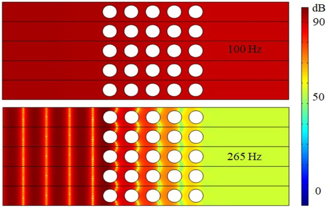
Total sound pressure contours for cylindrical scatterers, where, IL is around 0 dB at 100 Hz, and 34.5 dB is at 265 Hz.
C-shaped scatterers
The calculated band structure and IL for five rows of periodic C-shaped scatterers have been shown in Figure 6. The detailed observations made with IL for the for the periodic C-shaped scatterers have been tabulated in Table 1. The
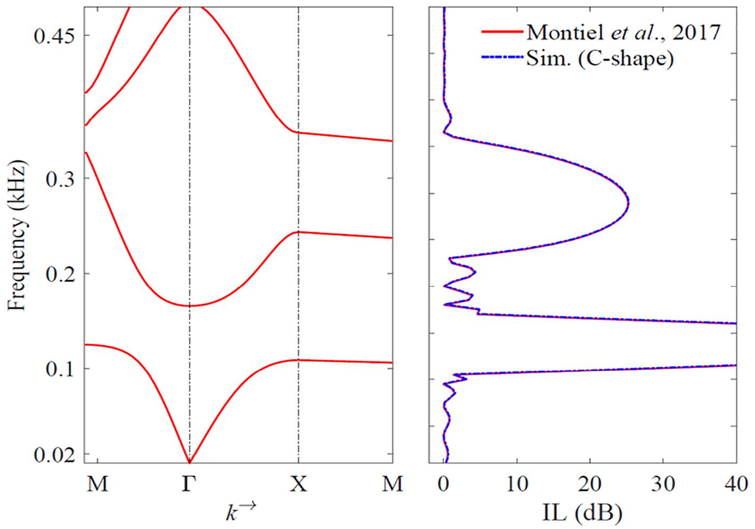
Calculated bandgap and IL of C-shaped scatterers.
Apart from the Bragg band, another peak has been observed, which is due to the resonance of the C-shaped scatterer, and can be noticed in Figure 6. The peak f1∞
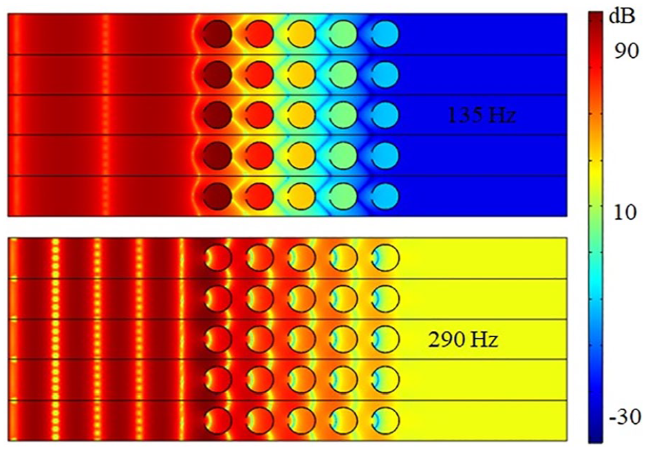
The total sound pressure contours for C-shaped scatterers, where,
The detailed observations with IL for the periodic cylindrical and C-shaped scatterers. The values of
Effect of Thermo-viscous Loss
Next, thermo-viscous losses have been considered to calculate the IL. Different geometry has been taken for calculating IL with considering thermo-viscous loss. The thermos-viscous effect plays a vital role when the boundary layer affects the air particle oscillations.
The first three rows of periodic cylindrical scatterers have been simulated with consideration of thermo-viscous loss in the frequency domain. The outer diameter (d) of the scatterers is 42 mm, arrange in a square lattice arrangement, where, the lattice constant (a) is taken as 67 mm.
Next, periodic C-shaped scatterers have been studied. The outer diameter (d) of the scatterer, shell thickness (t), slit width (w), and lattice constant (a) are 42, 3, 3, and 67 mm, respectively. The calculated IL with thermo-viscous loss has been shown in Figure 8. From Figure 8(a), it can be observed that by considering thermo-viscous losses no significant change has been observed in IL.
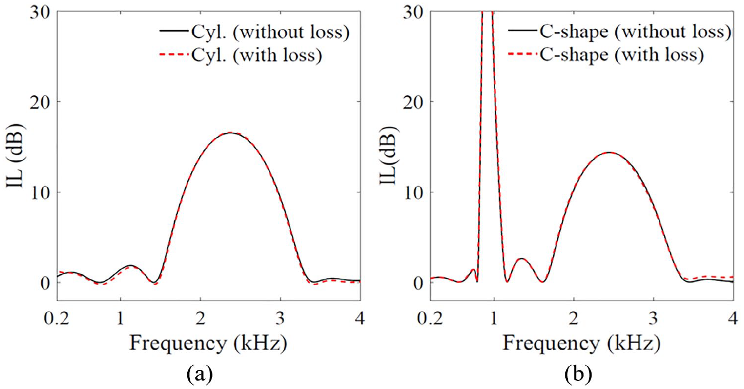
Calculated IL with thermo-viscous loss for; (a) periodic cylindrical scatterers, and (b) C-shaped scatterers.
For periodic C-shaped scatterers, the amplitude of resonance peak f1∞
Experimentation
At last, the experiments have been conducted in the laboratory environment. The schematic of the experimental setup, source, and receiver inside the portable anechoic chamber has been shown in Figure 9. The details of measurement and instrumentation are enumerated below.
(a) The measurement has been carried out inside a portable anechoic chamber of size (2 m×2 m×2 m), where, the background sound pressure is ≈30 dB(A) and the cutoff frequency is around 340 Hz. For the reference, other experimental studies also have been performed using portable anechoic chamber.26–28
(b) The sound pressure has been measured with PCB© free field array microphone. The calibration of the microphone has been carried out with an L&D© class one calibrator with (model no CAL-200©).
(c) The National Instruments (NI) data acquisition system has been used for measurement. It consists of an analog input module (NI©-9234) and an analog output module (NI©-9363). The modules are mounted on a chassis and connected to the host computer via USB connectivity. The LabVIEW© application software has been developed and used for IL measurement.
(d) A full range Daytron© speaker has been used here, which is a Gaussian white noise point sound source. In the numerical studies incident plane wave is used because the distance between the source to periodic scatterers is more than lambda (λ) of frequencies of interest. The point source is driven by an Ahuja© sound amplifier. The noise is generated using the LabVIEW© software and fed to the power amplifier via analog output.
(e) Scatterers are placed in between the source and the receiver. The microphone has been kept 0.25 m close to the periodic scatterers to avoid lateral passage of sound. The point noise source has been placed 2 m away from the receiver microphone. The acoustic signal has been captured at 51,200 samples/second to calculate the SPL (sound pressure level).
(f) The IL is measured in the direction of wave propagation or
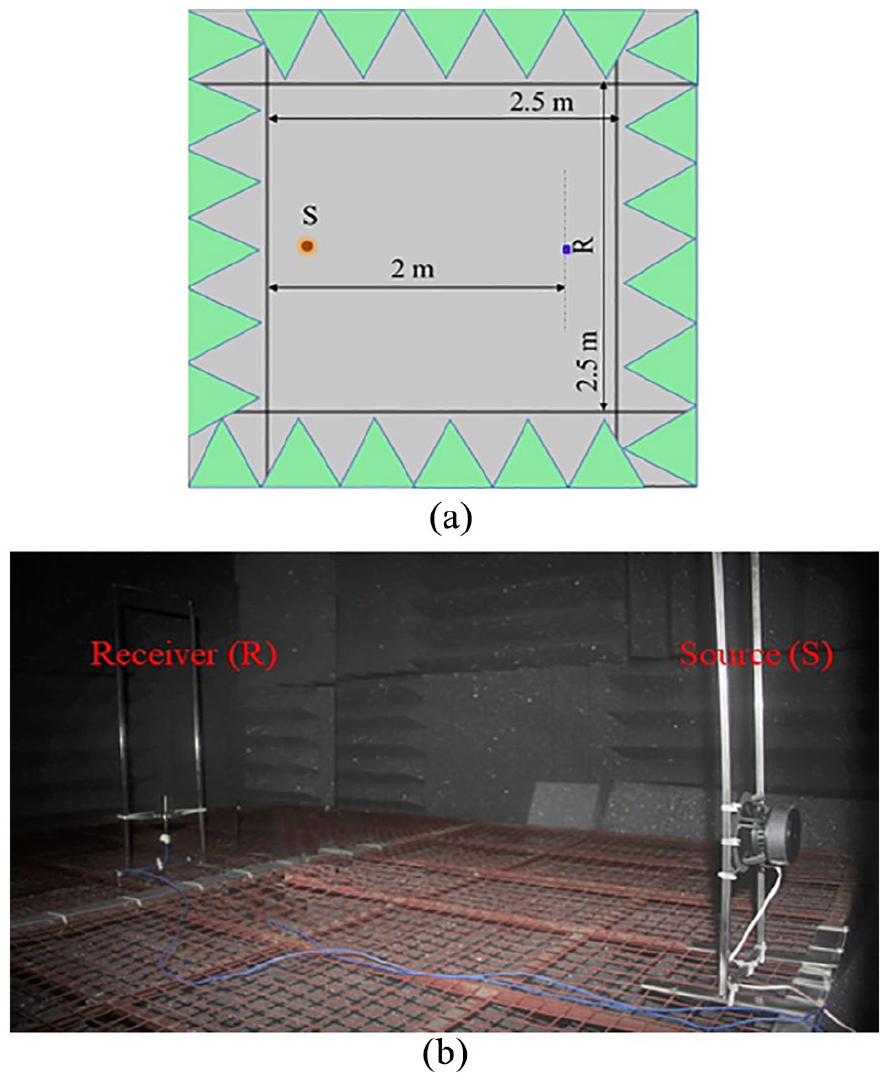
Experimental set up; (a) schematic of experiment, and (b) source and receiver inside anechoic chamber.
Fabrication of Scatterers
For the experiment, a finite size of periodic cylindrical and C-shaped scatterers has been prepared. The said periodic scatterers are comprised of 18 scatterers, where, there are three rows and six columns. All scatterers are made with PVC (Polyvinyl Chloride) pipe with an outer diameter of 42 mm and shell thickness of 3.5 mm. The approximate density of the PVC pipe is around 1400 kg/m3.
The scatterers are mounted on a plywood sheet of thickness 10 mm in a square lattice structure. The lattice constant (a) is 67 mm. The C-shaped scatterers are having slit width (w) of 3 mm. All machining operations have been done using an MTAB© CNC machine in the laboratory environment. Similarly, the scatterers have been mounted on a plywood panel using glue.
During fabrication, the parallel spacing of scatterers, and perpendicular mounting of scatterers have been taken care of. The prepared test sample of cylindrical scatterers and C-shaped scatterers is shown in Figure 10(a) and (b), respectively.
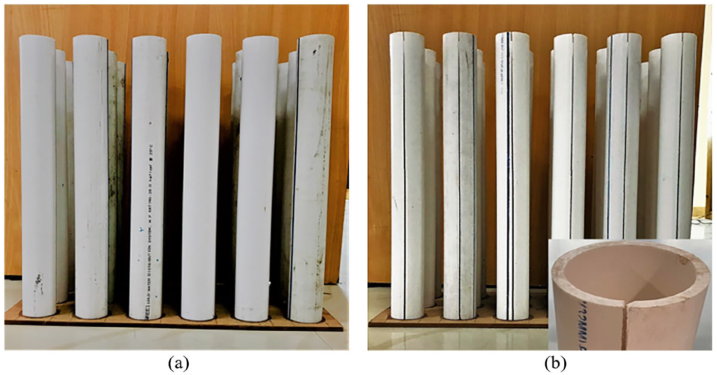
Fabricated sample of periodic; (a) cylindrical scatterers, and (b) C-shaped scatterers (top view of C-shaped scatterer with slit is shown in right of bottom corner).
Measurement of insertion loss
The experimental setup for measuring IL of periodic cylindrical and C-shaped scatterers has been shown in Figure 11(a) and the 2D schematic of the IL measurement is shown in Figure 11(b). Positions of the microphone and speaker are shown in the same figure. The receiver (microphone) is placed close to the post periodic scatterers to avoid the lateral passage of sound and sound can pass through the periodic scatterers. The acoustic panels having a thickness of 25 mm have been placed on three sides of the periodic structure during measurement to minimize the effect of edge diffraction, which has been shown in Figure 12(a) and (b), respectively.
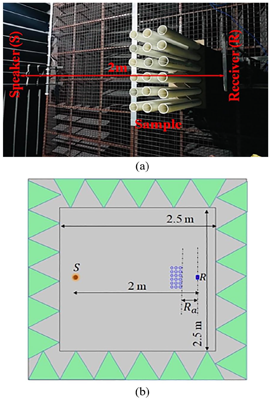
Experimentation; (a) Source and receiver location with respect to periodic scatterers, (b) 2D schematic of the IL measurement.
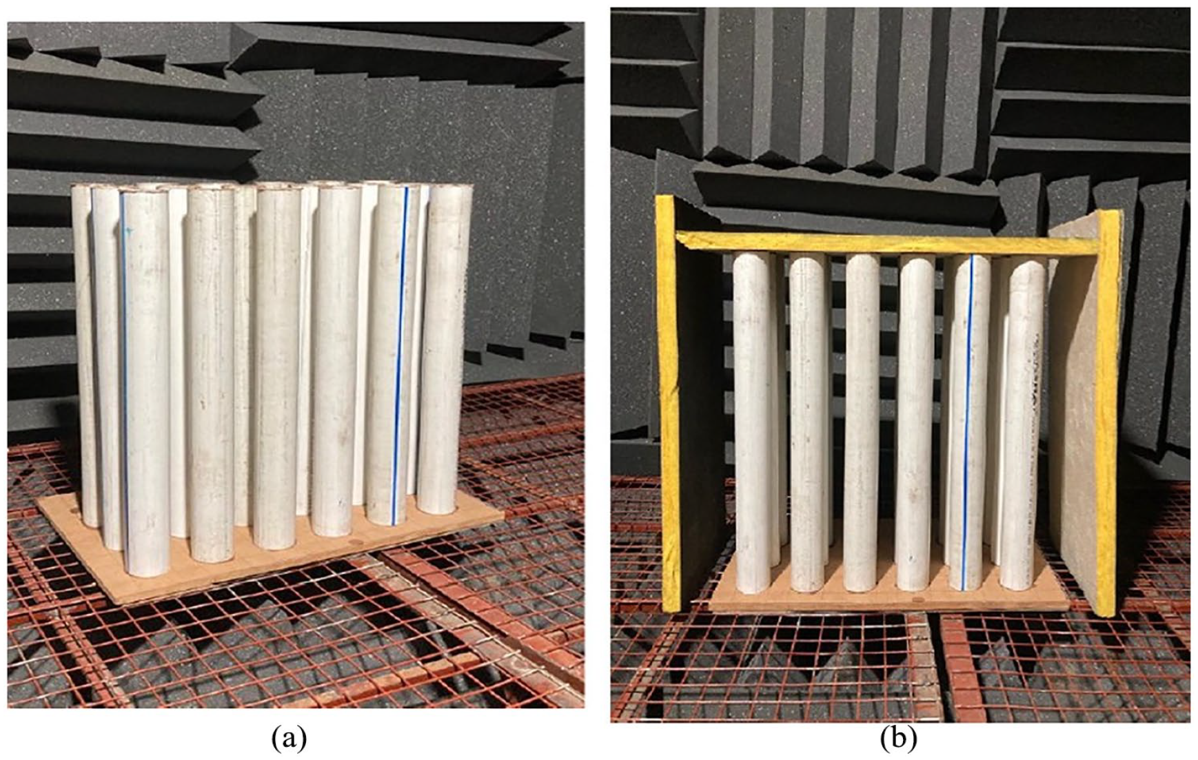
Periodic cylindrical scatterers and test environment; (a) without acoustic panel, and (b) with acoustic panel.
The measured IL of three rows of periodic cylindrical scatterers has been shown in Figure 13. Bragg band
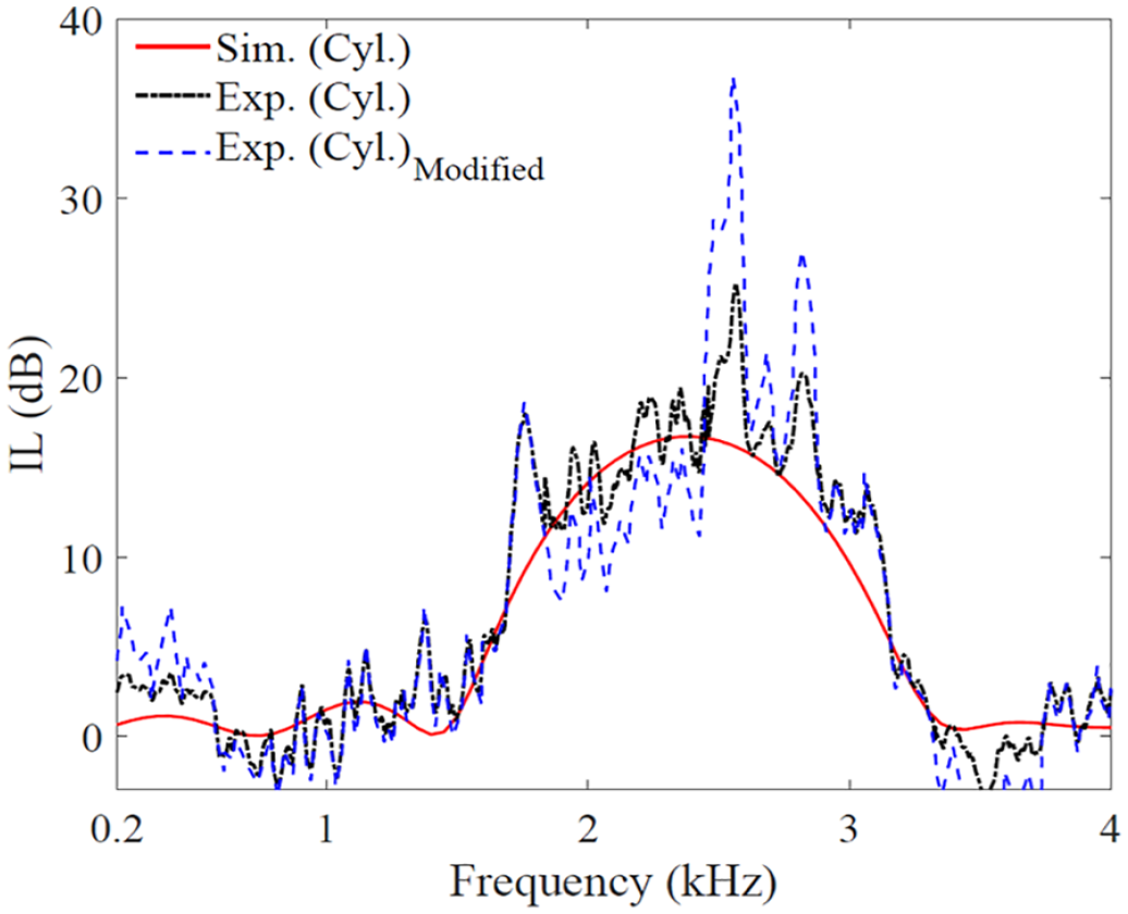
Calculated and measured IL with given test environments, where, diameter of cylindrical scatterer (d) = 42 mm, height of scatterers is 500 mm, and square lattice constant (a) = 67 mm.
The calculated IL of periodic C-shaped scatterers is shown in Figure 14, it can be seen that the IL of periodic C-shaped scatterers has two major band gaps. One additional peak is corresponding to the local resonance of the C-shaped scatterers.
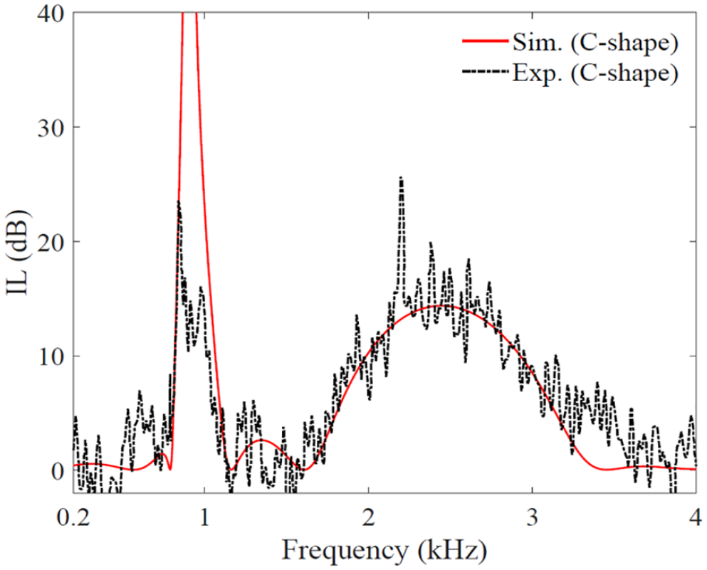
Calculated and measured IL with given test environments, where, diameter of cylindrical scatterer (d) = 42 mm, height of scatterers is 500 mm, and square lattice constant (a) = 67 mm), thickness oh shell (t) = 3.5 mm, and width of slit opening (w) = 3 mm.
The observed fluctuations in the Bragg band and resonance band may be due to the elastic properties of the PVC material which is not completely rigid, noise floor in the measurement which is about ≈30 dB(A), and the low and nonlinear source strength of sound source (combined speaker and amplifier). Moreover, the structural material and the structural losses have not been included in the simulation.
Conclusion
Using the suggested simulation technique the calculated IL for periodic cylindrical and C-shaped scatterers agrees with the results reported by Montiel et al. 25 The Bragg band is the range of frequency attenuation for periodic cylindrical scatterers. However, an additional peak apart from the Bragg band is observed in the lower frequency regime for C-shaped resonant scatterers, which is due to the resonance of scatterers. For cylindrical scatterers, one band gap is observed due to the periodicity of the scatterers named Bragg band gap. However, two band gaps named as resonant band gap and Bragg band gap are observed using C-shaped scatterers. The IL calculated with consideration of thermo-viscous loss has a minute or negligible variation with respect to results obtained from simulations with a lossless wave equation. The experiment with a finite size of periodic scatterers agrees with the results obtained from the simulation and can be used to authenticate the observations made with simulations.
Footnotes
Declaration of conflicting interests
The author(s) declared no potential conflicts of interest with respect to the research, authorship, and/or publication of this article.
Funding
The author(s) received no financial support for the research, authorship, and/or publication of this article.