Does the party in power affect FDI? First causal evidence from narrow margin US state elections

Abstract

Does the party of government influence the amount and type of inward foreign investment? Correlational studies provide inconsistent evidence. Moreover no existing study, for any level of government or any jurisdiction, uses methods that allow for causal inference. We apply regression discontinuity methods to a set of narrow margin US gubernatorial elections. Over the course of a 4-year term the election of a Republican governor causes a 17% boost in the growth of manufacturing-oriented FDI stock, compared to a Democrat. However, the same approach provides no evidence that partisanship matters for the overall level of FDI.

Keywords

foreign direct investment (FDI)partisanship political economy regression discontinuity design (RDD)US politics

Introduction

Political leaders—local and national—are not reticent in taking credit for investment flowing into their jurisdictions. This is not surprising given that foreign direct investment (FDI) contributes significantly to the vitality of most modern economies. The ability to attract and retain outside investment is often an important part of the prospectus of candidates from both major parties in US gubernatorial elections.

Foreign investors make their investment decisions in a very complex environment. They are typically less informed about the local policy environment when operating abroad and may be treated differently than domestic investors (Bhattacharya et al., 2007). Additional layers of rules and regulations associated with national boundaries such as capital controls and differential tax treatments may be imposed on foreign investment (Julio and Yook, 2016). Moreover, foreign investment is hard to be reversed without paying high costs (Rivoli and Salorio, 1996). As a result, FDI is more sensitive to the regulatory environment than domestic investment.

The literature on FDI determinants documents a number of factors multinational companies consider. The traditional factors may include, market size and growth potential (Resmini, 2000), industry clustering (Wheeler and Mody, 1992), labor market flexibility and financial depth (Yu and Walsh, 2010), infrastructure (Blonigen and Piger, 2014; Dunning, 1998). More recent literature points out that in addition to cost-benefit calculations, foreign direct investment could be explained more broadly by social ties of firm managers or diaspora networks (Bandelj, 2011; Leblang, 2010).

Moreover, the political factors, such as taxes, policy instruments, regulations, governmental institutions can influence the local business climates and subsequently firm location decisions (Fox, 1996). For example, as the largest single investment in Tennessee’s history, Nissan’s assembly plant investment in 1982 is an example illustrating the promotional role of the state. Lamar Alexander, a Republican who was governor of Tennessee when Nissan opened its factory in Tennessee made many efforts to encourage this investment. In fall of 1979, shortly after his inauguration, Lamar Alexander flew to Japan to meet Nissan executives and show the advantages of Tennessee. Nissan finally agreed to locate in Tennessee, and at the same time, Tennessee spent 12 million USD for new roads to the facility, and provided a 7 million USD grant for training plant employees and a 10 million USD county tax break (Kotabe, 1993). When Nissan came to Tennessee, there were almost no auto jobs in the state and 30 years later, one-third of the manufacturing jobs in Tennessee are auto-related. This is regarded as one of Alexander’s biggest accomplishments as governor.

The political parties are important to FDI decisions as they have implications for foreign investment relevant policies such as tax and other financial incentives as well as other policies that are applicable to both domestic and foreign firms such as industry regulations. These policies can affect the risk and return of the foreign investment.

While there are many some correlational studies relating the political “type” of those holding office to the vigor of FDI into states, countries and cities, there is no empirical evidence (from the US or anywhere else) of any causal link. This is the gap that we seek to fill in this paper. More concretely our research question is: Are Democrat or Republican state Governors better at attracting FDI?

The empirical evidence on the matter is mixed. Using a pooled cross-section data, Halvorsen and Jakobsen (2013) find that on average FDI is higher in Republican governed states. That effect is not statistically significant, however, leading them to conclude that “…foreign direct investors seem relatively agnostic with respect to the question of which party controls the state government” (p. 182). McMillan (2009) finds a significant and positive relationship between Democratic governorship and FDI. Using a slightly different measure Fox (1996) also finds a positive and significant association between Democratic governorship and the foreign firm location decisions.¹ With a focus on national governments Pinto and Pinto (2008) argue that government’s partisanship should affect foreign investors’ decision to flow into different sectors of the host country. In particular jurisdictions with left-leaning governments experience greater inflow into sectors where investment can be expected to be good to labor, since left-leaning governments cater to labor. While right-leaning governments are likely to attract foreign investment that would flow into those sectors where FDI could help increase the rents of domestic businesses. The central problem with existing studies such as these is that they point only to correlations and are unable to speak to issues of causation. This is a big limitation. For example, states that have unobserved characteristics that predispose them to elect Republican governors also have characteristics (perhaps the same characteristics, perhaps others) that make them attractive targets for inward investment. At the same time there may be causal effects running in the opposite direction. A state that is successful in attracting much foreign investment might (for whatever reason) develop economically or socially in a way that makes it more likely to vote for a particular type of leader.

We apply a regression discontinuity design (RDD) to a set of narrow margin gubernatorial elections between 1977 and 2004 to generate the first evidence of a causal link from the party affiliation of the governor of a state to the level and pattern of FDI that flows into that state.² The identifying assumption that underpins the application of RDD to close elections is that when one party or the other wins by a sufficiently narrow margin then the partisanship of the victory can be regarded as being (close to) random (Eggers et al., 2015; Lee, 2008).

In brief our results are as follows. The election of a Republican as governor has a statistically significant positive effect on net FDI inflows in manufacturing industries to a state. The effect is substantial—17% in aggregate dollars in our preferred specification—and is sustained throughout the term of office. Interestingly it makes no significant difference to the total value of FDI inflow. The results are relatively undisturbed by inclusion or exclusion of a range of controls, and prove robust to a variety of robustness tests.

We will point to various strands of related literature (de la Cuesta and Imai, 2016; Eggers et al., 2015; Grimmer et al., 2011). However we deliberately exclude claims of the channels through which party affiliation might matter. Indeed one attraction of the RDD method is that it allows the researcher to remain agnostic as to the mechanism or mechanisms at play. The powers of a Governor are manifold, and the partisanship of the officeholder might influence investment flows through various channels. Some of these might be direct, such as inducements and trade visits. Others indirect. Foreign investors may be attracted to places with low taxes, flexible regulators, promise a responsive workforce or offer cohesive social settings (Head et al., 1999).

There are often-claimed partisan differences in approach to economic policy which might influence the type of investor to which a state appeals. The party affiliations of politicians can reflect the kinds of policies that states adopt to promote economic development (Quinn and Shapiro, 1991). Ideology-induced policies are especially prevalent at state level in the US (Potrafke, 2018).

Republicans generally prefer an investment-driven growth model that pursue investment through direct business-friendly approaches. Available tools at state level for direct measures include various forms of tax incentives, direct grants or subsidies for business, state programs to promote R&D, low-interest loans, subsidized training of employees and cheap access to land. Also, prior studies find evidence that Republican governors are more active in deregulating labor markets (Bjørnskov and Potrafke, 2013) and less active in protecting environment (Beland and Boucher, 2015).

Democrats are likely to favor a consumption-driven growth model that seek to encourage investment through indirect, redistributive measures. Indirect measures involve a preference for higher taxation and higher government spending. In terms of allocation of state expenditures, Democratic governments are associated with higher spending in education, health and public safety sectors and lower spending on natural resources and highways (Beland and Oloomi, 2017). In addition, under Democratic governors, states have a higher minimum wage, lower post-tax inequality and unemployment rate (Leigh, 2008).

The rest of the paper is organized as follows. The second section describes methods and data. The third section reports results. The final section concludes.

Research design

In this section we outline our methods and data sources, including discussion of assumptions and potential challenges to compelling identification.

Methods

Early applications of regression discontinuity method to close election datasets demonstrated the possibility of incumbency advantage (Lee, 2008), policy responsiveness (Lee et al., 2004) and the rents from holding office (Eggers and Hainmueller, 2009). Several authors have used the method to explore the effects of partisanship on other economic outcomes. For example, Ferreira et al. (2009), Gerber and Hopkins (2011) and de Benedictis-Kessner and Warshaw (2016) present corresponding empirical evidence on close US mayor election and the size of government. Innes and Mitra (2015) looked at election and regulatory outcomes; Beland (2015) at labor market outcomes; and Leigh (2008) at numerous policy settings, including minimum wage, post-tax inequality, and unemployment rate.

Our preferred results rely on the nonparametric local polynomial estimation methods due to Calonico et al. (2014). The method fits a weighted polynomial function to observations above and below the discontinuity within a particular bandwidth. The polynomial function usually takes order 1 or 2, and the weights are determined endogenously, not by researcher discretion, by a kernel function that performs the computation based on the distance of observations from the discontinuity. Within the bandwidth, the closer the observation is to the discontinuity the more heavily it is weighted.

The steps in estimation are as follows.

First, a bandwidth h is selected. The bandwidth is the width of the interval around the discontinuity within which the local polynomial is fitted. Typically this choice has been made arbitrarily, and for election-based studies has been set at 5% or 10% winning margins (Beland, 2015; de la Cuesta and Imai, 2016; Erikson et al., 2015). In choosing bandwidth the researcher faces a trade-off between bias and variance.³ We follow the procedure developed in Calonico et al. (2014) for choosing the optimal bandwidth—that which minimizes the asymptotic mean squared error (MSE) of the regression discontinuity estimator, where MSE is the sum of the bias squared and variance of the estimator. The choice of optimal bandwidth also means that we avoid ad hoc decisions and the risk of (conscious or inadvertent) specification searching.

Second, a kernel function $K (\cdot)$ is chosen. The function assigns non-negative weights to each observation x_i around the cut-off c and within the bandwidth. The commonly used kernel function is the triangular kernel function which applies more weight to observations closer to the cut-off. Using the kernel function we compute a weight w_i for each observation where

w_{i} = K ((x_{i} - c) / h)

Third, weighted least squares regression is run separately on the set of observations that are above the cut-off but within the bandwidth and those below the cut-off but within the bandwidth on the choice of the polynomial. The order of the polynomial should be kept low and high order of the polynomials tends to lead to approximation error due to the overfitting and biases at the boundary points (Skovron and Titiunik, 2015).

Finally, we take the difference of the two estimated intercepts and get the regression discontinuity estimate. In effect the size of the “jump” in the outcome variable that occurs at the discontinuity. Once we get the point estimate, we are interested in constructing the confidence interval and testing the hypothesis. Under the MSE optimal local polynomial estimation, the conventional inference method has been shown to be invalid (Skovron and Titiunik, 2015), so we adopt the robust confidence intervals proposed in Calonico et al. (2014).

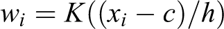
To implement the local linear version we fit weighted linear regression functions to the observations within a bandwidth h on either side of the cut-off point c. In other words,

\begin{array}{l} \underset{α_{1}, β_{1}}{minimize} & \sum_{i : c - h < x_{i} < c} {(y_{i} - α_{1} - β_{1} (x_{i} - c))}^{2} w_{i} \end{array}

and

\begin{array}{l} \underset{α_{2}, β_{2}}{minimize} & \sum_{i : c < x_{i} < c + h} {(y_{i} - α_{2} - β_{2} (x_{i} - c))}^{2} w_{i} \end{array}

Given the estimates of ${\hat{α}}_{1}$ and ${\hat{α}}_{2}$ , the estimated average treatment effect is

{\hat{τ}}_{r d} = {\hat{α}}_{2} - {\hat{α}}_{1}

In this paper, we estimate the local treatment effect, following the methodology proposed by Calonico et al. (2014). The local-linear regression offers flexibility with little loss of statistical power. We have adopted what we believe to be current best practice in RDD to model the relationship between assignment and outcome variable, using local-linear estimation with an optimal MSE (mean-square-error), bandwidth and robust confidence intervals.

Study setting

States are the primary subdivisions of the US and have a high degree of autonomy in how they govern themselves. State governor controls the governmental budget, appoints many officials, and has a plethora or other powers. Governors can veto bills and, in many cases, have the power of the line-item veto on appropriation bills. In addition to hard authority, the governor can also bring to bear significant “soft” power through the authority given to him/her by his/her office. In summary, governors are influential players in US politics.

A governor may run his/her state in a way that makes it more or less attractive to a prospective international investor. In addition, in recent decades they have been increasingly visible players on the international scene. External state-promotional activity dates back to the 1970s (Fry, 1998; Watson, 1995) and has focused on promoting trade and attracting inward investment. As regards FDI in particular, states take the lead role in recruitment of inward investment, with the role of the federal government much smaller. Many state-operated international offices and governor-led overseas missions are set up to attract FDI (McMillan, 2009). US state officials claim that the international trade and investment is the largest category of state international engagement (Whatley, 2003). As a result, the governor of a state acts as the chief economic “ambassador” in appealing to prospective investors.

Data

We obtain data from several sources. Our outcome variable of interest is FDI. State-level FDI data is drawn from US Bureau of Economic Analysis. We first obtain the total monetary amount of FDI stock and the FDI stock in manufacturing sectors in each US State for each year from 1977 to 2004. The FDI stock refers to the real book value of gross property, plant, and equipment (PPE) of all nonbank affiliates. This includes the value of buildings, structures, machinery, and equipment, etc. but excludes inventories and intangible assets. It corresponds to the standard definition of FDI in the US. We are interested in FDI flows, so we take the difference between the FDI measures in the year governor was elected (elections almost always occur in November) and each of the 4 years following where governor took the office respectively. So for example, if the governor wins a close election in November 2005 we take the difference between FDI stock in 2005 with that stock in 2006, 2007, 2008 and 2009. This allows us to answer four slightly different questions: How much “extra” FDI does a governor of a particular political persuasion attract in his first year in office, first 2 years in office, etc. In most cases the fourth variant can be taken to approximate the extra FDI across the whole term in office. In addition, taking changes in the outcome variable (rather than working with levels) serves to increase the statistical efficiency of our regression discontinuity design (Lee and Lemieux, 2010).

Table 1 presents summary statistics for FDI and other covariates. The mean FDI stock per capita across the whole of the US is 2796 USD and the mean FDI stock per capita in the manufacturing sector 921 USD.

Table 1.

Summary statistics.

	Mean	Std. Dev	Min	Max
	(1)	(2)	(3)	(4)
FDI Stock per Capita	2795.70	4972.94	71.77	47463.41
FDI Stock per Capita in Manufacturing	920.82	1017.17	16.61	8322.05
FDI Stock / GSP	0.112	0.143	0.009	1.844
FDI Stock in Manufacturing / GSP	0.041	0.036	0.002	0.275
GSP Growth Rate	3.205	3.910	−18.571	31.576
Corporate Tax Rate	6.823	2.873	0	12.25
Population	4986858	5483532	397363	35842038
Union	15.741	7.142	2.8	38.3
Wage	13.454	1.740	9.589	21.329
Education Expense	32.889	6.268	15.957	50.201
Farm Land	41	24.3	1	93
Urbanization	71.70	14.76	38.2	94.4

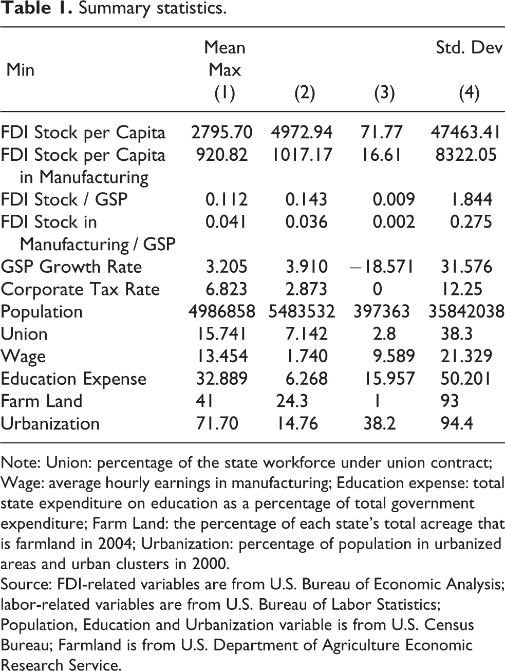
Note: Union: percentage of the state workforce under union contract; Wage: average hourly earnings in manufacturing; Education expense: total state expenditure on education as a percentage of total government expenditure; Farm Land: the percentage of each state’s total acreage that is farmland in 2004; Urbanization: percentage of population in urbanized areas and urban clusters in 2000.

Source: FDI-related variables are from U.S. Bureau of Economic Analysis; labor-related variables are from U.S. Bureau of Labor Statistics; Population, Education and Urbanization variable is from U.S. Census Bureau; Farmland is from U.S. Department of Agriculture Economic Research Service.

The data on gubernatorial elections are obtained from two sources. The election data from 1977 to 1990 is drawn from dataset Candidate and Constituency Statistics of Elections in the United States, 1788–1990 (ICPSR 7757) from the Inter-university Consortium for Political and Social Research. The remaining election data comes from Dave Leip’s Atlas of U.S. Presidential Elections (Leip, 2008).

Gubernatorial elections usually take place in November and the governor elected takes power in the following January. A governor’s term usually is 4 years.⁴ We define the election margin to be the percentage of votes obtained by the Republican candidate minus the percentage obtained by the Democrat. Following that convention the discontinuity is at zero (we can ignore third candidates). If the election margin is positive (negative), the Republican (Democrat) has won.

Table 2 summarizes outcomes in the 361 elections in our sample. Of those Republicans won 186, Democrats won 175 times. In terms of close elections we count for the purpose of this summary table those with winning margins of 5% and 10%. Within a 5% interval around the cut-off, we get 81 elections of which Republicans won 42 times, Democrats won 39 times. Of the 157 elections within 10% of the cut-off Republicans won in 80, Democrats in 77. So by each of these metrics the sample is roughly balanced, no party seems systematically more likely to prevail when result margins are narrow. If we look at the elections in terms of incumbents and challengers, we can see that incumbents win more often. However, in the case of close elections, the winning frequency of incumbents and challengers are balanced. Incumbents won rough same number of times as challengers in 5% margins, while challengers won slightly more times in 10% margins. The close-to-symmetric shape of the barchart of density of winning margins in Figure 1 is consistent with this. Together these numbers suggest that there is no precise manipulation of selection into the treatment, which would threaten the validity of the identification assumption on which application of the RDD rests. To back-up this “eye-ball” test, we will conduct and present the results of more formal tests later.

Figure 1.

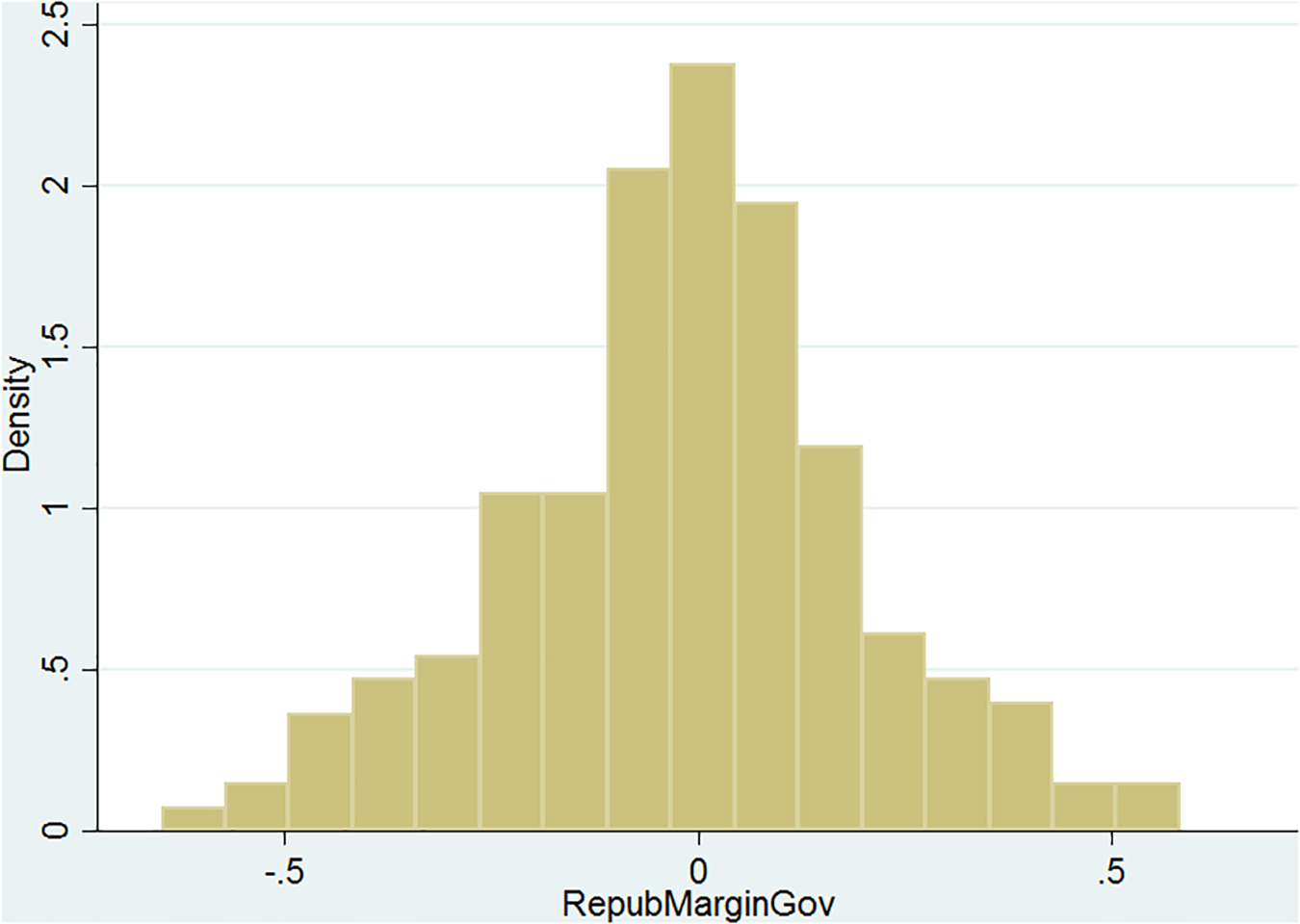
Margins of victory.

Table 2.

Statistics on gubernatorial elections.

Number of Elections	5%	10%	Total
All elections	81	157	361
Republican won	42	80	186
Democratic won	39	77	175
Incumbent won	41	74	222
Challenger won	40	83	139

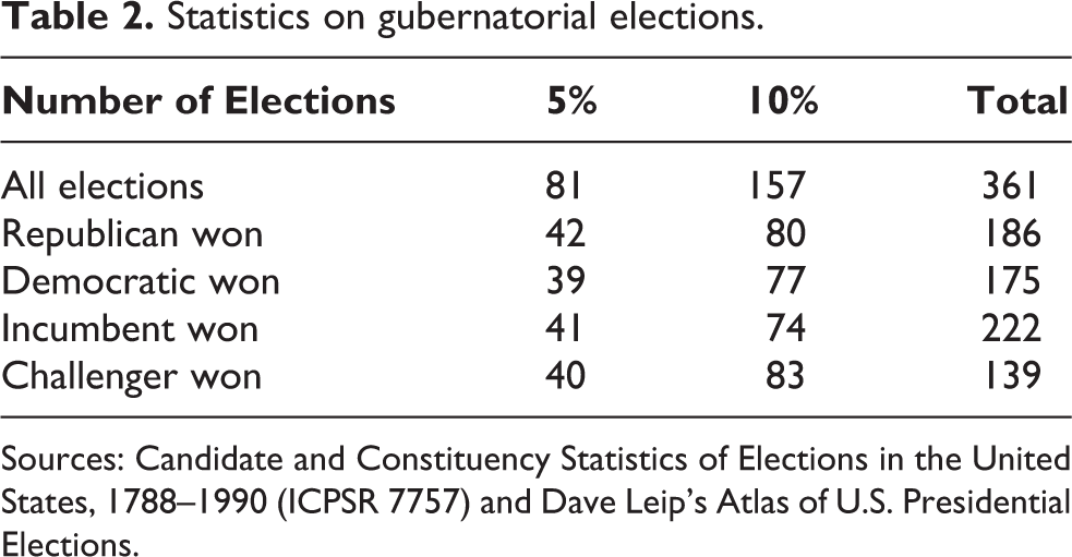
Sources: Candidate and Constituency Statistics of Elections in the United States, 1788–1990 (ICPSR 7757) and Dave Leip’s Atlas of U.S. Presidential Elections.

To improve precision other control variables are included. We control for a number of factors that could affect the attraction of FDI. First, previous studies have found that rapid economic growth in the host economy stimulates greater demand for FDI inflows (Kang and Jiang, 2012). We include the growth rate of gross state product to capture the economic condition. Higher corporate taxes are expected to deter investment (Wijeweera et al., 2007). Thus, we include state’s corporate tax rate. The labor market conditions have been included in some previous studies (Sethi et al., 2003). We therefore include percentage of the state workforce under union contract and average hourly earnings in manufacturing, which takes into account the cost and quality of the labor. In addition, we also include population, farmland and urbanization, which plausibly could affect FDI decisions. Farmland is the percentage of each state’s total acreage that is farmland in year 2004 and urbanization refers to the percentage of population in urbanized areas and urban clusters in the year 2000.

Data for the control variables are obtained from several sources. The labor-related variables are from U.S. Bureau of Labor Statistics. Figures for educational expenditures and urbanization are from U.S. Census Bureau. Farmland is from the U.S. Department of Agriculture Economic Research Service.

Results

Main results

Tables 3 and 4 present main results on the causal impact of the election of a Republican on (1) FDI per capita and (2) FDI in manufacturing per capita. Significance levels are adjusted by robust inference methods proposed by Calonico et al. (2014). The robust p-values are regarded as conservative, so the significance of the results reported will also hold if we were to use conventional p-values. Standard errors are clustered at state level.

Table 3.

RD estimates for FDI per capita.

	One year after election			Two years after election
	(1)	(2)	(3)	(1)	(2)	(3)
Repub won	88.38 (114.89)	58.83 (109.49)	136.32 (106.5)	245.47** (144.82)	235.94** (149.07)	164.68 (163.71)
Bandwidth	0.180	0.209	0.168	0.131	0.135	0.126
Party Change		✓	✓		✓	✓
Controls			✓			✓
Effective Observations	215	237	195	171	177	162
Total Observations	341	341	334	336	336	329
	Three years after election			Four years after election
	(1)	(2)	(3)	(1)	(2)	(3)
Repub won	80.09 (225.01)	55.00 (230.11)	89.24 (229.5)	−197.73 (272.41)	−131.58 (278.62)	−139.57 (263.25)
Bandwidth	0.179	0.199	0.167	0.193	0.192	0.212
Party Change		✓	✓		✓	✓
Controls			✓			✓
Effective Observations	186	201	169	192	192	199
Total Observations	305	305	301	299	299	295

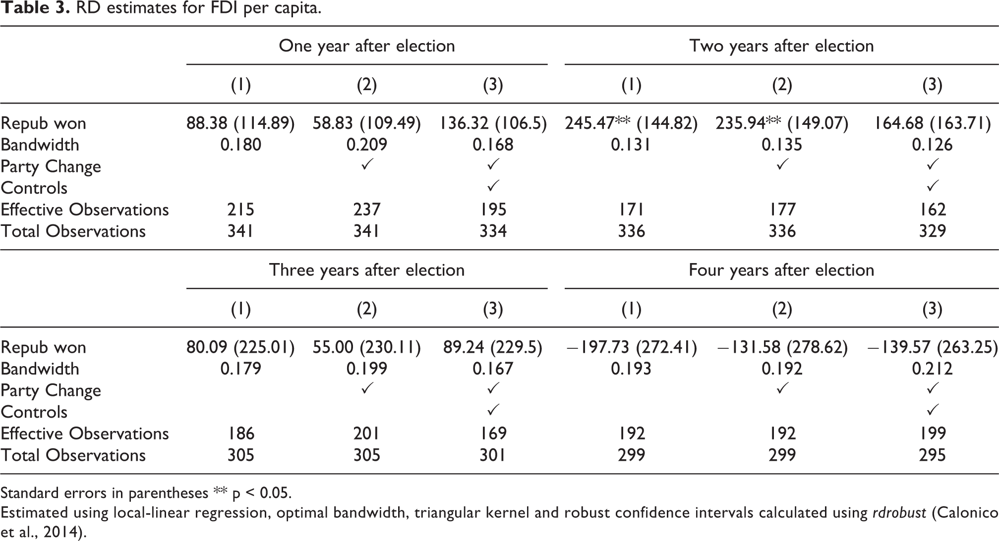
Standard errors in parentheses ** p < 0.05.

Estimated using local-linear regression, optimal bandwidth, triangular kernel and robust confidence intervals calculated using rdrobust (Calonico et al., 2014).

Table 4.

RD estimates for FDI manufacturing per capita.

	One year after election			Two years after election
	(1)	(2)	(3)	(1)	(2)	(3)
Repub won	103.04*** (38.706)	102.84*** (38.193)	84.28*** (30.135)	177.56*** (59.49)	176.31*** (59.394)	131.07*** (48.458)
Bandwidth	0.072	0.074	0.081	0.076	0.077	0.082
Party Change		✓	✓		✓	✓
Controls			✓			✓
Effective Observations	95	98	97	100	100	100
Total Observations	303	303	299	301	301	297
	Three years after election			Four years after election
	(1)	(2)	(3)	(1)	(2)	(3)
Repub won	240.06*** (59.21)	242.18*** (59.034)	239.88*** (51.329)	145.97** (66.121)	144.53** (65.789)	156.89*** (59.889)
Bandwidth	0.110	0.110	0.105	0.115	0.115	0.111
Party Change		✓	✓		✓	✓
Controls			✓			✓
Effective Observations	126	125	118	129	129	123
Total Observations	288	288	284	284	284	280

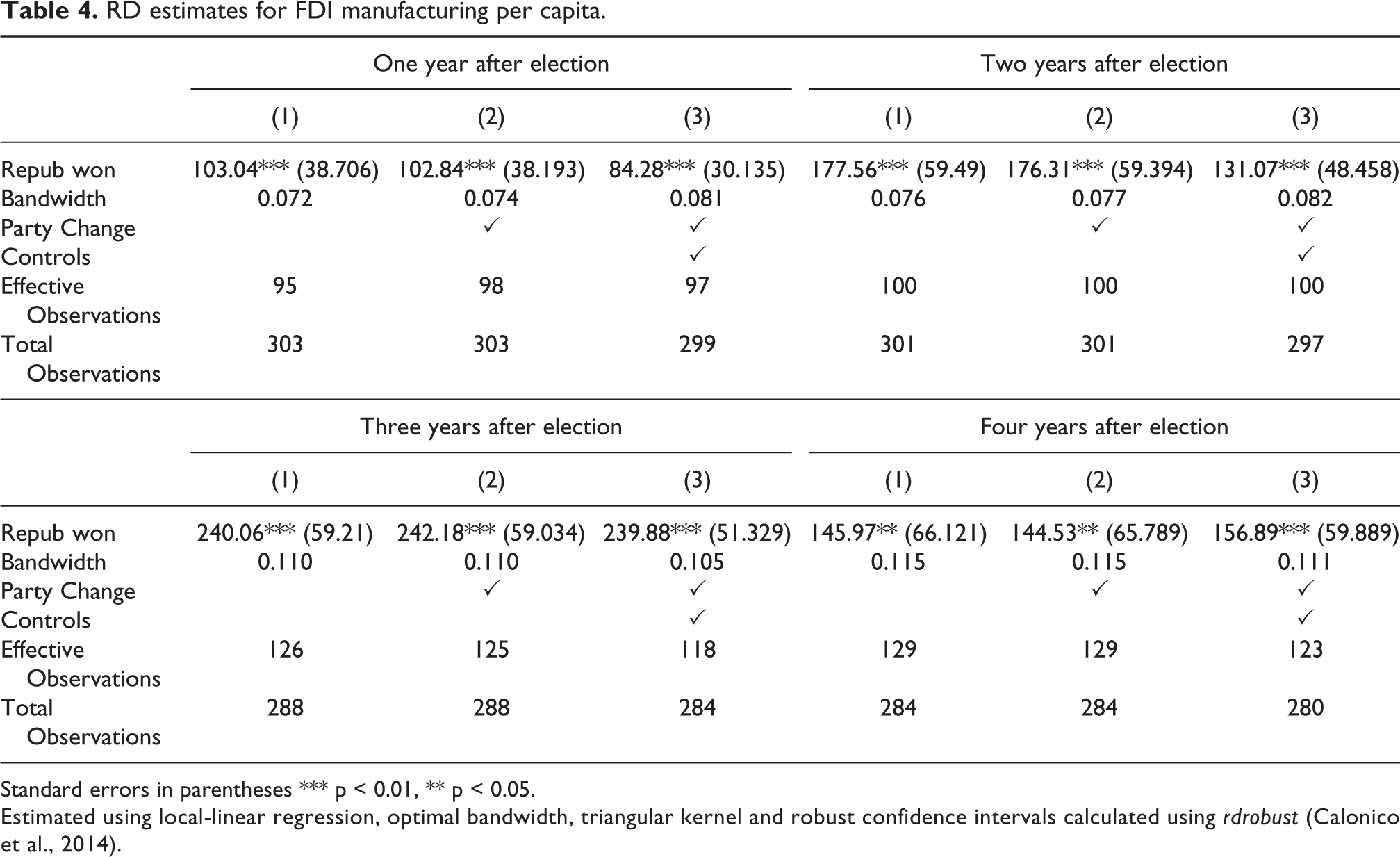
Standard errors in parentheses *** p < 0.01, ** p < 0.05.

Estimated using local-linear regression, optimal bandwidth, triangular kernel and robust confidence intervals calculated using rdrobust (Calonico et al., 2014).

Table 3 relates to FDI per capita. The top number in each column is the estimated discontinuity—the additional FDI causally attributed to a Republican win. In each panel, column (1) derives from estimates with no controls. Column (2) includes a control for whether the election was associated with a change in ruling party. Column (3) adds party change and other controls. The estimates are generally not significant. The second panel identifies a positive and significant effect of a Republican win on FDI inflow in the 2-year window following an election win, but the value becomes smaller and significance is lost (even at 10%) once controls are added. Overall the analysis reported in Table 3 points to no discernible effect, positive or negative, of a Republican governorship.

Table 4 reports the results of conducting the same exercise but specialized on flows of FDI per capita into the manufacturing sectors. We find a significant positive effect of a Republican governor on these flows, which can be interpreted causally. The effect sustains whole term of governor. The results are relatively insensitive to exclusion or inclusion of the control for party change or other controls.

Panel 1 implies that in his/her first year in office a Republican governor, other things equal, attracts an additional 84.28 USD dollars of FDI in manufacturing per head compared to his/her Democratic counterpart. In the first 2 years he/she attracts an additional 131.07 USD. In his/her first 3 years an additional 239.88 USD is attracted. And in the full 4 years of his/her term an additional 156.89 USD is attracted. Note that these are not “within year” flows, but rather the cumulative effect over four different time horizons. The state-level average FDI per capita in manufacturing in our sample is 920.82 USD so against that benchmark, the growth in FDI stock in manufacturing activities is 17% higher under a Republican governor during a 4-year term compared to a the counter-factual of a Democratic governor.

Figures 2 and 3 plot the estimates RD estimates of the effects of a Republican governorship on cumulative FDI per capita (Figure 2) and FDI in manufacturing per capita (Figure 3) across each of the four time horizons. The plotted estimates are based on our preferred specifications with all controls and the confidence levels are presented at 90% and 95%.

Figure 2.

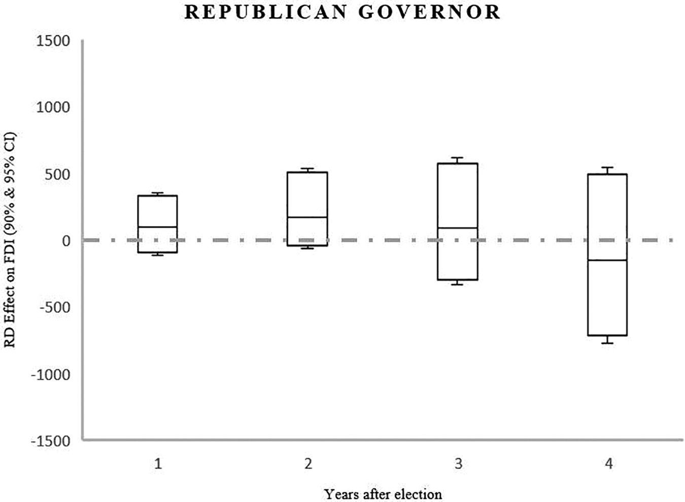
RD estimates on FDI, 1 to 4 years after election. Note: The plotted estimates are based on the preferred specifications with all controls and the confidence levels are presented at 90% and 95%.

Figure 3.

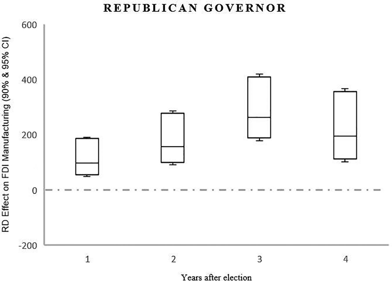
RD estimates on FDI manufacturing, 1 to 4 years after election. Note: The plotted estimates are based on the preferred specifications with all controls and the confidence levels are presented at 90% and 95%.

Figure 4 present the fitted curves either side of the discontinuity for each of the four exercises (recall that each exercise refers to a different time horizon over which the impact of the governorship on cumulative FDI is assessed). The “jump” in the vicinity of the discontinuity is the effect presented in the earlier tables, and it can be seen here to be positive in each of the four panels. The size of each dot is determined by the number of election data points in each winning margin bucket. While the specifications reported are estimated over a wider interval, we can see comparatively large dots in the immediate vicinity either side of the discontinuity, and that visually there is a very apparent step up from those just to the left of the discontinuity to those just to the right. While the data points further from the discontinuity are included in the estimates, they carry correspondingly lower weight.

Figure 4.

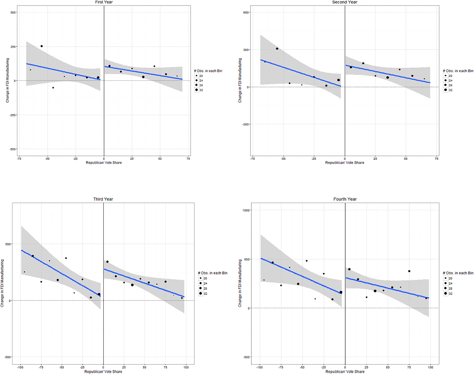
The effect of electing a Republican governor on change in FDI in manufacturing. Note: The vote share is multiplied by 1000. The black dots are averages in 0.5% bins and shaded are 95% confidence intervals.

To summarize; (1) we find no evidence that the political affiliation of the state governor has a causal impact on total FDI inflow. However, (2) there is a significant (at 1%), positive and substantial effect of a Republican governorship on inflows of manufacturing FDI, an effect that is sustained across the whole of the governor’s term in office.

Puzzlingly, we only find significant effects on manufacturing FDI rather than total FDI. One potential explanation is that manufacturing industries are likely to differ from non-manufacturing industries with respect to their sensitivity to election outcomes.⁵ While it is difficult to classify industries as being politically sensitive or not, there are some guidance from the political economy literature. Herron et al. (1999) attempt to identify 15 economic sectors as politically sensitive by using measures of candidate electoral prospects based upon the Iowa Electronic Market during the 1992 Presidential election. Top three politically sensitive sectors in Herron et al. (1999) are pollution control sector and aerospace and defense, pharmaceuticals. Also, when analyzing the relationship between political uncertainty and corporate investment cycles, Julio and Yook (2016) classify firms in tobacco products, pharmaceuticals, health care services, defense, petroleum and natural gas, telecommunications, and transportation industries as politically sensitive. The industries identified as politically sensitive in the above studies are mostly concentrated in manufacturing industries. In addition to the sensitivity of industries, the other reason might be that one particular target of state economic development efforts has been the foreign manufacturing firms (Fox, 1996).

Validity

In this section, we challenge our study design by performing three validity checks.

A key assumption of RDD is the continuity assumption—that the only change which occurs at the point of discontinuity is the shift in the treatment status.⁶ This would be compromised if, for example, one party or the other were able to manipulate the winning margin such as to be “just over the line.” In our setting, the violation of the continuity assumption would require the eventual winner be able to predict vote shares with extreme precision and then deploy necessary resources to win the close elections. Existing evidence suggests that this is not a significant risk in our setting (de la Cuesta and Imai, 2016; Eggers et al., 2015). However, the following validity checks confirm that there is no evidence of such sorting behavior.

The standard approach to challenging the random selection into treatment assumption is the McCrary test (McCrary, 2008). The McCrary test essentially tests for whether there is discontinuity in the density of the assignment variable in the vicinity of the discontinuity being used for identification. The McCrary graph is presented in Figure 5. If the parties can manipulate the election results in close elections, we should expect the proportion of observations just to the left of the cutpoint to be meaningfully different from those to the right. Sorting, if it exist, would produce a discontinuity in the density of the forcing variable. We can easily see that the density is smooth around the cut-off and there is no unusual jump. Consistent with Erikson et al. (2015) and Eggers et al. (2015), we find no significant discontinuities in the gubernatorial election, suggesting that there is no evidence of sorting.

Figure 5.

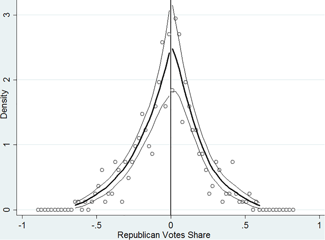
McCrary density of victory margin.

We also conduct the density test proposed by Cattaneo et al. (2015), another continuity-based test of design. It uses a local polynomial density estimator that does not require the pre-binning of the data and leads to a size and power improvement (Skovron and Titiunik, 2015). We are able to reject the null hypothesis that the density is discontinuous at the cut-off with an associated P-value of 0.4496.

To further examine whether the key identification assumption of the RD design is credible, we conduct tests on a number of covariates. In particular, we perform the estimation on the covariates following the same methodology, and the results are presented in Table 5 and we find no significance for all covariates except corporate tax rate.⁷ The corporate tax rate is significantly lower under republican governors. This could be a channel that how republican governors attract more foreign investment. For other covariates, the results show that party affiliation of the governor has no effect on these variables.

Table 5.

Covariate balance tests for gubernatorial RD design.

	Estimate	BW	CI	Pr > \|z\|	N
GSP Growth Rate	0.654	0.147	(−2.888, 4.604)	0.653	273
Corporate Tax Rate	−0.601	0.168	(−1.354, −0.074)	0.029	309
Population	94453	0.142	(−199154, 486529)	0.411	345
Union	−0.597	0.142	(−2.845, 1.808)	0.662	309
Wage	−0.111	0.119	(−0.658, 0.608)	0.939	305
Education Expense	−0.429	0.195	(−1.910, 1.437)	0.782	309
Farm land	−4.475	0.160	(−25.522, 14.323)	0.582	363
Urbanization	5.188	0.147	(−4.531, 18.136)	0.239	363

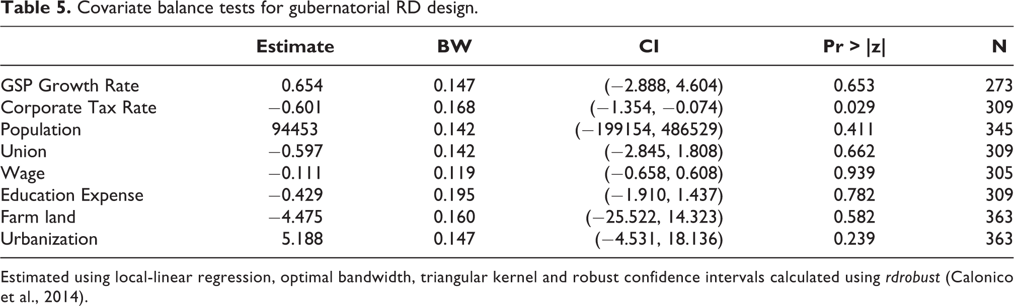
Estimated using local-linear regression, optimal bandwidth, triangular kernel and robust confidence intervals calculated using rdrobust (Calonico et al., 2014).

Methodological robustness

In the main results section we explored the robustness of our main estimates to exclusion and inclusion of a variety of state-level controls. In this section, we perform sensitivity tests to examine the robustness of our RDD results as they apply to FDI in manufacturing to changes in modeling assumptions.⁸

Senate/house and president

In our preferred specification, we add state and time-varying characteristics including state population, percentage of the state workforce under union contract, average hourly earnings in manufacturing, unemployment rate, education expenses, farmland and urbanization in order to control for possible confounding factors that might influence the results.

To better isolate the impact of the gubernatorial election, we include more factors that may play roles in shaping foreign economic policies. In addition to state governor, state legislatures are also regarded powerful on international issues (McMillan, 2009). In Table 6 we include the variables indicating which party controls the house and which controls the senate. Also, the party holds office at national level matters for setting the economic climate. In Table 6 we control that the variables indicating which party the president belongs to. The results are robust to the inclusion of dummy variables for having Republicans control the state senate, for Republicans controlling the state house, and for the president being a Republican.

Table 6.

RD estimates for FDI manufacturing per capita: senate/house/president.

	One year after election		Two years after election
	(1)	(2)	(1)	(2)
Repub won	79.50*** (30.267)	91.55*** (30.373)	126.15*** (49.366)	128.76*** (48.234)
Bandwidth	0.084	0.080	0.082	0.082
Party Change	✓	✓	✓	✓
Controls	✓	✓	✓	✓
Senate/House	✓		✓
President		✓		✓
Effective Observations	97	100	95	100
Total Observations	291	299	289	297
	Three years after election		Four years after election
	(1)	(2)	(1)	(2)
Repub won	268.81*** (56.777)	255.16*** (52.092)	172.33*** (63.793)	185.74*** (59.714)
Bandwidth	0.088	0.099	0.103	0.100
Party Change	✓	✓	✓	✓
Controls	✓	✓	✓	✓
Senate & House	✓		✓
President		✓		✓
Effective Observations	98	115	112	113
Observations	276	284	273	280

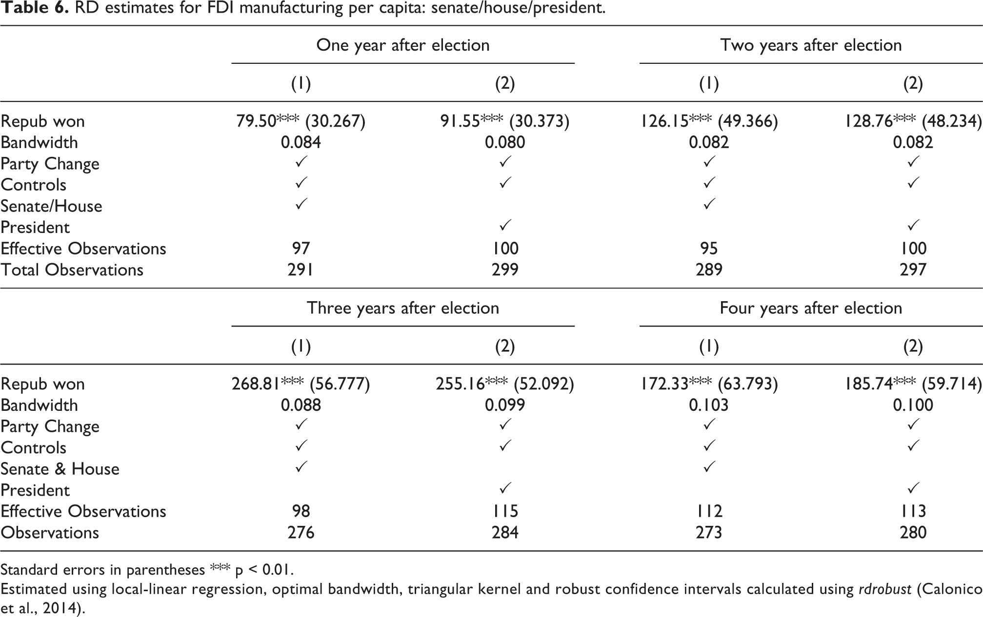
Standard errors in parentheses *** p < 0.01.

Estimated using local-linear regression, optimal bandwidth, triangular kernel and robust confidence intervals calculated using rdrobust (Calonico et al., 2014).

Governor characteristics

Since 1980, partisan differences have grown rapidly in the US states. The parties have increasingly diverged in the policies they implement in office. Republican governors do pursue different policies compared to Democrats (Caughey et al., 2016). However the existing evidence show that the educational and occupational background of leaders may have impacts on outcomes. For example, Besley et al. (2011) show that heterogeneity among leaders’ educational attainment is important with growth being higher by having leaders who are more highly educated. Neumeier (2018) finds that the tenures of US state governors with a business background are associated with higher annual income growth rate, higher growth rate of the private capital stock, and lower unemployment rate.

In Table 7, we control for the educational and occupational background of state governors.⁹ Specifically, we include three dummy variables. Political experience is a dummy variable taking the value 1 if the incumbent governor is politically experienced (0 otherwise), which is defined as having held any elected political office at the local, state, or federal level before the current position. Business experience is a dummy variable taking the value 1 if the governor was a businessperson prior to entering politics and 0 otherwise. Education background is an indicator whether a governor has low education, i.e. less than a Master’s degree. The results are presented in Table 7. We can see that our main results are not significantly disturbed by controlling for the educational and occupational background of state governors.

Table 7.

RD estimates for FDI manufacturing per capita: governor characteristics.

	One year after election	Two years after election
Repub won	91.56*** (33.732)	131.65*** (49.115)
Bandwidth	0.124	0.09
Party Change	✓	✓
Controls	✓	✓
Governor Characteristics	✓	✓
Effective Observations	134	102
Observations	287	285
	Three years after election	Four years after election
Repub won	240.92*** (53.041)	166.61*** (64.648)
Bandwidth	0.100	0.104
Party Change	✓	✓
Controls	✓	✓
Governor Characteristics	✓	✓
Effective Observations	108	109
Observations	273	269

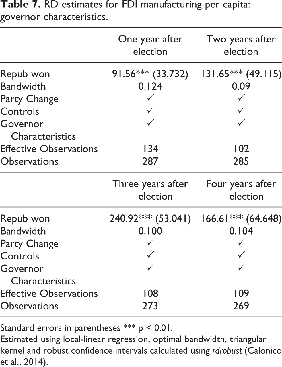
Standard errors in parentheses *** p < 0.01.

Estimated using local-linear regression, optimal bandwidth, triangular kernel and robust confidence intervals calculated using rdrobust (Calonico et al., 2014).

Bandwidth

For our preferred estimates we adopted an optimal bandwidth following Calonico et al. (2014). The optimal bandwidth selected by the method varies between about 7% and 10% across the specifications. This is similar to the bandwidth chosen (usually arbitrarily) in other applications of RDD methods to close elections.¹⁰ Nonetheless, as robustness checks we re-run each regression imposing first a 5% and then a 10% bandwidth. The results of these exercises are presented in Table A1. The estimates retain sign and significance and are similar in value to those from the preferred specifications in Table 4.

Order of polynomial

In our base specification we fitted the data linearly on either side of the discontinuity. This is the preferred approach because Gelman and Imbens (2014) argue that estimators for causal effects based on high-order (third, fourth, or higher) polynomials can be misleading in the RDD setting. Gelman and Imbens (2014) recommend instead use estimators based on local linear or quadratic polynomials.

In Table A2 we report the results of repeating the exercise but fitting a second-order polynomial. Again we can see that the size of the estimated effects are little disturbed, and in all cases the sign and significance of the effect is sustained.

Outliers

In Table A3, we address whether the results of our main regressions are driven by the more industrialized ones. The average share of manufacturing sector in state GDP in our sample is 16%. The four big industrialized states in our sample are North Carolina (30%), Indiana (28%), Michigan (27%), Ohio (25%). We re-estimate our preferred specification but excluding four big industrialized states. It can be seen that the results are similar to the baseline results, suggesting that geographical heterogeneity does not bias the results.

To further allay concerns that the result is being driven by a small number of extreme observations we perform outlier analysis by winsorizing data at 99% and 95% level. Winsorization is the statistical transformation of the data by limiting extreme values in the data to reduce the effect of (possibly spurious) outliers (winsorization is widely used by economists (Alesina et al., 2015; Dick and Lehnert, 2010). A 99% winsorization, for example, would see all data below the first percentile set to the 1st percentile, and data above the 99th percentile set to the 99th percentile. Winsorization methods are usually more robust to outliers, although there are alternatives, such as trimming, that will achieve a similar effect. One advantage of winsorization is that the transformation limits the impact of outliers, without losing observations. The results are presented in the Table A4. The results are little disturbed by the winsorization suggesting that they are not overly driven by a few extreme-valued outliers.

Alternative denominator for dependent variable

Our central analysis took as dependent variable FDI per capita as out measure of FDI intensity. An alternative and equally sensible approach would have been to work with FDI per unit of percentage of state-level GSP. To confirm that this would not significantly have disturbed conclusions we re-estimate our preferred specification on that basis. The results of this exercise are reported in Table A5.

In this version, a Republican governor—compared to the benchmark of a Democrat—causes a 11% increase in FDI stock in manufacturing as a percentage of the gross state product after 1 year and an increase of 27% over the 4-year term in office. These are qualitatively similar to our main results, though somewhat larger in size.

Conclusion

Foreign investment plays a crucial role in the American—and other—economies. But how influential is the type of government in a place in determining the levels or patterns of inward investment?

In this paper, we present what we believe to be the first empirical investigation of a causal link from political partisanship to FDI. As such we provide a further empirical point-of-connection between political and economic outcomes, with a direction of effect. To obtain plausibly exogenous assignment of treatment (political party in power) we use a regression discontinuity design, exploiting the discontinuity generated by the first-past-the-post election system.

The evidence points to Republican governors causing a substantial and sustained upward bump in foreign investment into manufacturing activities, when compared to their Democratic counterparts. However, we find no evidence one way or the other on total FDI flows, although those effects are much less precisely estimated.

There are some limitations of this study. One limitation of our research design is that the effects are identified by the subset of gubernatorial election whose vote outcome is close to the majority threshold. The limitation of such a design is that we are only able to identify a causal relation locally. Extending the external validity of this study by identifying natural experiments that apply to a broader universe of party politics and FDI is an exciting and challenging avenue for future research. Another limitation is that we only explore the aggregate level of FDI. A fruitful extension of this study is to explore the partisan effects on more finely classified activities—which types of economic activity are more or less sensitive to political events than others?

Supplemental material

Supplemental Material, sj-docx-1-ppq-10.1177_13540688211030108 - Does the party in power affect FDI? First causal evidence from narrow margin US state elections

Supplemental Material, sj-docx-1-ppq-10.1177_13540688211030108 for Does the party in power affect FDI? First causal evidence from narrow margin US state elections by Kunyu Wang and Anthony Heyes in Party Politics

Footnotes

Author's Note

Anthony Heyes is also affiliated with University of Exeter, UK.

Declaration of conflicting interests

The author(s) declared no potential conflicts of interest with respect to the research, authorship, and/or publication of this article.

Funding

The author(s) received no financial support for the research, authorship, and/or publication of this article.

ORCID iD

Kunyu Wang

Supplemental material

Supplemental material for this article is available online.

Notes

References

Alesina

Cassidy

Troiano

(2019). Old and young politicians. Economica 86(344): 689–727.

Angrist

Pischke

J-S

(2008) Mostly Harmless Econometrics: An Empiricist’s Companion. Princeton, NJ: Princeton university press.

Bandelj

(2011) Relevance of nationality in cross-border economic transactions. Nationalities Papers 39(6): 963–976.

Beland

L-P

(2015) Political parties and labor market outcomes: evidence from US states. American Economic Journal: Applied Economics 7(4): 198–220.

Beland

L-P

Boucher

(2015) Polluting politics. Economics Letters 137: 176–181.

Beland

L-P

Oloomi

(2017) Party affiliation and public spending: evidence from US governors. Economic Inquiry 55(2): 982–995.

Besley

Montalvo

Reynal-Querol

(2011) Do educated leaders matter? The Economic Journal 121(554): F205–227.

Bhattacharya

Galpin

Haslem

(2007) The home court advantage in international corporate litigation. The Journal of Law and Economics 50(4): 625–660.

Bjørnskov

Potrafke

(2013) The size and scope of government in the us states: Does party ideology matter? International Tax and Public Finance 20(4): 687–714.

10.

Blonigen

Piger

(2014) Determinants of foreign direct investment. Canadian Journal of Economics/Revue canadienne d’économique 47(3): 775–812.

11.

Calonico

Cattaneo

Titiunik

(2014) Robust nonparametric confidence intervals for regression-discontinuity designs. Econometrica 82(6): 2295–2326.

12.

Cattaneo

Jansson

(2020) Simple local polynomial density estimators. Journal of the American Statistical Association 115(531): 1449–1455.

13.

Caughey

Warshaw

(2017) Incremental democracy: The policy effects of partisan control of state government. The Journal of Politics 79(4): 1342–1358.

14.

de Benedictis-Kessner

Warshaw

(2016) Mayoral partisanship and municipal fiscal policy. The Journal of Politics 78(4): 1124–1138.

15.

de la Cuesta

Imai

(2016) Misunderstandings about the regression discontinuity design in the study of close elections. Annual Review of Political Science 19: 375–396.

16.

Dick

Lehnert

(2010) Personal bankruptcy and credit market competition. The Journal of Finance 65(2): 655–686.

17.

Dunning

(1998) Location and the multinational enterprise: A neglected factor? Journal of International Business Studies 29(1): 45–66.

18.

Eggers

Hainmueller

(2009) MPs for sale? Returns to office in postwar British politics. American Political Science Review 103(04): 513–533.

19.

Eggers

Fowler

Hainmueller

, et al. (2015) On the validity of the regression discontinuity design for estimating electoral effects: new evidence from over 40,000 close races. American Journal of Political Science 59(1): 259–274.

20.

Erikson

Folke

Snyder

(2015) A gubernatorial helping hand? How governors affect presidential elections. The Journal of Politics 77(2): 491–504.

21.

Ferreira

Gyourko

(2009) Do political parties matter? Evidence from US cities. The Quarterly Journal of Economics 124(1): 399–422.

22.

Fox

(1996) The influence of political conditions on foreign firm location decisions in the American states (1974-1989). Political Research Quarterly 49(1): 51–75.

23.

Fry

(1998) The Expanding Role of State and Local Governments in US foreign Affairs. New York, NY: Council on Foreign Relations Press.

24.

Gelman

Imbens

(2014) Why high-order polynomials should not be used in regression discontinuity designs. Technical report. Cambridge, MA: National Bureau of Economic Research.

25.

Gerber

Hopkins

(2011) When mayors matter: estimating the impact of mayoral partisanship on city policy. American Journal of Political Science 55(2): 326–339.

26.

Grimmer

Hersh

Feinstein

, et al. (2011) Are close elections random? Unpublished manuscript.

27.

Halvorsen

Jakobsen

(2013) Democrats, republicans or both? An empirical analysis of the effects of the composition of state governments on FDI, 1977–2004. International Interactions 39(2): 167–191.

28.

Head

Ries

Swenson

(1999) Attracting foreign manufacturing: investment promotion and agglomeration. Regional Science and Urban Economics 29(2): 197–218.

29.

Herron

Lavin

Cram

, et al. (1999) Measurement of political effects in the United States economy: a study of the 1992 presidential election. Economics & Politics 11(1): 51–81.

30.

Innes

Mitra

(2015) Parties, politics, and regulation: evidence from clean air act enforcement. Economic Inquiry 53(1): 522–539.

31.

Julio

Yook

(2016) Policy uncertainty, irreversibility, and cross-border flows of capital. Journal of International Economics 103: 13–26.

32.

Kang

Jiang

(2012) FDI location choice of Chinese multinationals in East and Southeast Asia: traditional economic factors and institutional perspective. Journal of World Business 47(1): 45–53.

33.

Klašnja

Titiunik

(2017) The incumbency curse: Weak parties, term limits, and unfulfilled accountability. American Political Science Review 111(1): 129–148.

34.

Kotabe

(1993) The promotional roles of the state government and Japanese manufacturing direct investment in the United States. Journal of Business Research 27(2): 131–146.

35.

Leblang

(2010) Familiarity breeds investment: diaspora networks and international investment. American Political Science Review 104: 584–600.

36.

Lee

(2008) Randomized experiments from non-random selection in us house elections. Journal of Econometrics 142(2): 675–697.

37.

Lee

Lemieux

(2010) Regression discontinuity designs in economics. Journal of Economic Literature 48(2): 281–355.

38.

Lee

Moretti

Butler

(2004) Do voters affect or elect policies? Evidence from the US house. The Quarterly Journal of Economics 119(3): 807–859.

39.

Leigh

(2008) Estimating the impact of gubernatorial partisanship on policy settings and economic outcomes: a regression discontinuity approach. European Journal of Political Economy 24(1): 256–268.

40.

Leip

(2008) Atlas of US Presidential Elections. Available at: http://www.uselectionatlas.org (accessed on 8 June 2016.

41.

McCrary

(2008) Manipulation of the running variable in the regression discontinuity design: a density test. Journal of Econometrics 142(2): 698–714.

42.

McMillan

(2009) Looking beyond the national level: foreign direct investment attraction in us states. International Interactions 35(2): 155–178.

43.

Neumeier

(2018) Do businessmen make good governors? Economic Inquiry 56(4): 2116–2136.

44.

Pinto

(2008) The politics of investment partisanship: and the sectoral allocation of foreign direct investment. Economics & Politics 20(2): 216–254.

45.

Potrafke

(2018) Government ideology and economic policy-making in the united states—a survey. Public Choice 174(1–2): 145–207.

46.

Quinn

Shapiro

(1991) Economic growth strategies: the effects of ideological partisanship on interest rates and business taxation in the United States. American Journal of Political Science 35: 656–685.

47.

Resmini

(2000) The determinants of foreign direct investment in the CEECS: new evidence from sectoral patterns. Economics of Transition 8(3): 665–689.

48.

Rivoli

Salorio

(1996) Foreign direct investment and investment under uncertainty. Journal of International Business Studies 27(2): 335–357.

49.

Sethi

Guisinger

Phelan

, et al. (2003) Trends in foreign direct investment flows: a theoretical and empirical analysis. Journal of International Business Studies 34(4): 315–326.

50.

Skovron

Titiunik

(2015) A practical guide to regression discontinuity designs in political science. American Journal of Political Science 2015: 1–36.

51.

Watson

(1995) The New Civil War: Government Competition for Economic Development. Westport, CT: Praeger Publishers.

52.

Whatley

(2003) State Official’s Guide to International Affairs. Washington, DC: Council of State Governments.

53.

Wheeler

Mody

(1992) International investment location decisions: the case of US firms. Journal of International Economics 33(1–2): 57–76.

54.

Wijeweera

Dollery

Clark

(2007) Corporate tax rates and foreign direct investment in the United States. Applied Economics 39(1): 109–117.

55.

Walsh

MJP

(2010) Determinants of foreign direct investment: a sectoral and institutional approach. Number 10-187. International Monetary Fund.

Supplementary Material

Please find the following supplemental material available below.

For Open Access articles published under a Creative Commons License, all supplemental material carries the same license as the article it is associated with.

For non-Open Access articles published, all supplemental material carries a non-exclusive license, and permission requests for re-use of supplemental material or any part of supplemental material shall be sent directly to the copyright owner as specified in the copyright notice associated with the article.

0.00 MB

0.02 MB