
Abstract
Our article investigates the dynamic interlinkages between financial development, tourism development and economic growth in the top 10 tourism destination countries. The knowledge of which series has a causal power to predict tourism can inform policy making about which country needs marketing support and additional investment for its tourism growth. Moreover, results will throw light on which countries are assisted by their ex ante economic and financial development and can thus evolve into a tourism hub through the aid of the general economic development characterizing a country and/or a flourishing financial environment. Our study has employed a battery of cointegration and Granger-causality methods, which prove the robustness of our results. Specifically, we rely on the augmented mean group estimator and the novel Fourier Toda-Yamamoto (FTY)-based Granger-causality test, whose advantage lies in taking into account sharp and smooth structural breaks and resilient to cross-sectional dependence. The FTY reveals that the tourism-led growth hypothesis is confirmed for the United States, Italy, the United Kingdom, and Russia, while economic growth Granger-causes tourism development in the United States only. The financial development growth hypothesis in confirmed only for Spain and the United Kingdom, while economic growth Granger causes financial development in the United States, Italy, the United Kingdom, and Russia.
Keywords
Introduction
The tourism–economic growth nexus is a field of tourism economics that attracts a lot of attention, because it can provide tourism stakeholders with information of the Granger-causal direction of tourism and economic growth, also in relation to other magnitudes of interest, so that they can foster all the economic, structural, and policy sides that favor tourism growth and eliminate all those factors that discourage it. Foremost, the tourism–economic growth nexus can contribute to forecasting the future of the tourism outcome, given the realization of other macroeconomic magnitudes. Thus, it is a quite eloquent field that is continuously updated and supplemented with new information that is generated through more sophisticated modeling techniques that can forecast with greater accuracy the evolution of tourism and its potential connectedness to economic growth.
There are basically four main outcomes that can be generated in the investigation of the tourism–economic growth nexus field: (i) the tourism-led growth hypothesis (TLGH), wherein economic growth is led by tourism, so the latter is a very important factor in the economy and should be supported so that economic growth is not put at stake, (ii) the economic growth-led hypothesis (EGLH), where economic growth leads tourism. This means that other sectors in the economy are vibrant and contribute to the development of the economy, which in turn contributes to the development of tourism. This situation applies to countries where tourism is not an important sector and is seriously dependent on the progress of the rest of the economic sectors, which generate most of the growth for that economy. In such a case, depending on the priorities of a government and whether the latter truly aims to establish a robust tourism sector or not, it must support the whole economy, so that this in turn positively boosts tourism. (iii) The third hypothesis concerns a mutual Granger-causal effect between economic growth and tourism growth, whereby one magnitude affects the other and vice versa in a spiral effect. (iv) The fourth hypothesis concerns the neutrality case where the two magnitudes appear not to be connected in any way under a Granger-causal relationship.
The fact that tourism is not one single product, but rather a sum of relationships and services, what is termed as an “amalgama” in the relevant literature of tourism definition (Burkart and Medlik, 1974), for this reason its measurement has not been internationally stipulated either and it takes place in various ways and not as a single measure. Tourism can be measured with tourist arrivals, overnight spent, tourism expenditure, or tourism revenue or sometimes all of them, for reasons of comparison (Menegaki et al., 2020). However, a novelty of the current study is that it employs a tourism development index following Shahzad et al., (2017) with principal component analysis (PCA), which is a quintessential synthesis of the most important magnitudes of tourism and thus the dilemma and experimentation about which of the tourism demand measurement variables to use, is neatly addressed.
The relationship of tourism with financial development has been little documented as such (Katircioglou et al., 2018), but the common knowledge is that it contributes positively to the development of an economy as a whole and to specific economic sectors. Thus, our article contributes to and updates this scant literature too. Most importantly, our article has used novel Granger-causality methodologies, which have never been applied in the field so far. These novel methods are resilient to cross-sectional dependence, auto-correlation and structural breaks. Comparing our results with others from relevant studies, we claim that the Fourier Toda-Yamamoto (FTY) methodology has provided neat and smart results avoiding the over-validation of the TLGH. After this brief introduction, the remainder of our article is structured as follows: The second section offers a multistranded literature review, the third section describes the methodology, the fourth section includes the results with their discussion, while the fifth concludes the article.
Conceptual literature review
Due to the intersectional nature of our study (tourism and financial sector) and the fact that international tourism is a part of foreign trade, this literature review contains six subsections to facilitate a conceptual overview of the seminal and up-to-date literature:
The benefits from a good financial sector in an economy
In essence, financial development refers to the size of capital flows in financial institutions, capital markets and foreign direct investment (FDI). Financial development also influences environmental quality through the aforementioned mechanisms, but it should be remembered that environmental quality also affects tourism and is affected by tourism. When financial intermediation is efficient, not only tourism businesses can borrow at cheaper rates but also consumers can borrow to finance some of their costly items such as holiday packages. It has been stated in Levine (2002) that banks play their role in improving economic growth at initial levels of economic development and particularly under weak institutional environments on the condition that this does not lead to domestic capital leakages and the subsequent fragilities (Ahmed, 2013) that the weak institutional environment can impart to the system. The latter occurs, because banks offer services such as project evaluation, savings mobilization through various schemes of terms and interest rates, risk diversification and sharing, and transaction intermediation. These services help create the environment of safety necessary for technological progress and economic development to flourish. Financial development promotes economic growth, that is, capital accumulation and total factor productivity. Financial liberalization results in the improvement of the monetary transmission mechanism and this encourages savings and investment and then increases economic growth (Beakert et al., 2005).
The level of financial development induces economic growth by directly increasing savings in the form of financial assets, thereby spawning capital formation and hence economic growth (King and Levine, 1993). There is a bulk of studies that investigate the Granger-causal relationship between the financial sector and economic growth and these studies can be distinguished first on the basis of those that support the “demand-following” hypothesis, according to which financial development exists when it is demanded. Thus, poor countries with low levels of consumption and entrepreneurship do not need banks. On the other hand, the “supply-following” hypothesis supports that the existence of a financial system is a prerequisite for economic growth. Last, FDI brings in more competition for tourism and more innovation. The latter is very important for a tourism sector that needs not only to be more environmentally sustainable but also more technologically innovative through the extended usage of robotics, artificial intelligence, and other smart technologies. Overall, financial markets contribute to economic development through the enhancement of economic efficiency by diverting funds from unproductive uses to productive ones (Durusu-Ciftci et al., 2017). Financial deregulation through liberalization measures is also a significant factor in contributing to economic growth. The theoretical relationship between the variables is still unclear and this justifies further research towards this direction. Foremost, the financial sector stimulates the tourism producer’s activities and increases consumer’s purchasing power (Table 1).
Financial development channels affecting tourism activity.
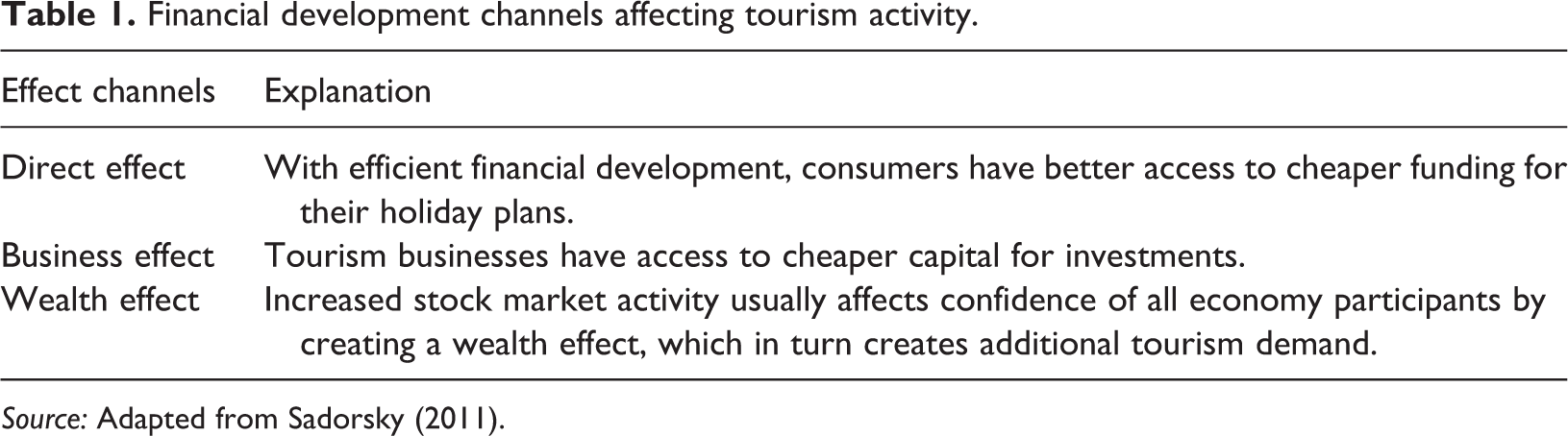
Source: Adapted from Sadorsky (2011).
A financial sector that operates efficiently can provide capital at lower interest rates and costs. Besides other sectors within the economy, this benefit is transmitted to investment in tourism as well. Financial development improves the opportunity to use new technology, helps businesses to adopt clean and environment-friendly production, and this improves global environment and regional development and sustainability (Birdsall and Wheeler, 1993; Frankel and Rose, 2002). For one thing, an improved financial sector can provide the tourism sector with funds to make environmental friendly tourism investments, introduce renewable energies, and improve the energy efficiency of hotels. Funds can also be directed to reduce seasonality in the tourism sector and build all-weather facilities that will encourage tourists to go on holiday irrespective of whether it is the season of year that they normally prefer. Cheap funds will also help tourism adopt all available new technologies that improve the tourism product, decrease production costs, and increase customer satisfaction.
Not much academic work has been done until today on the relationship of financial development and tourism development. In a chronological order, there are studies referring mostly on developing countries: Song and Lin (2010) for Asian countries, Kumar and Kumar (2013) for Fiji islands, Kumar (2014) for Vietnam, Basarir and Cakir (2015) for five Mediterranean countries, Ridderstaat and Croes (2015) for Aruba and Barbados, Shahbaz et al. (2016) for Malaysia, Ngoasong and Kimbu (2016) for Cameroon, and Katircioglu et al. (2018) for Turkey. The results of the above studies are shared between evidence for growth effects and evidence for feedback effects, namely that the financial sector has a positive causal effect to the development of tourism or that both tourism and financial sectors have causal effects to each other. Conversely, to the scant empirical work on the aforementioned relationship, there is, however, abundant empirical work on the relationship of trade and financial development from which some lessons can be brought forward and learned for tourism, which is a form of external trade. This is so because international tourism is a part of international trade and contributes essentially to the formation of balance of payments, when tourism is a large part of the economy.
Lessons from the relationship of financial development with international trade
International trade openness together with financial development are very important drivers of economic growth (Beck, 2002; Sachs and Warner, 1995). According to the theoretical model of Blackburn and Hung (1998), both the financial development and international trade liberalization increase economic growth. Trade openness also affects financial development (Beck, 2002). According to Rajan and Zingales (2003), when a country opens its borders to trade and capital flows, it is more likely to benefit from this dual openness, because both can promote competition and threaten the states of the incumbents. Beck (2002) has found that countries with a more developed financial system also enjoy a higher export share. There is various empirical evidence (Kim et al., 2010a, 2010b; Svaleryd and Vlachos, 2002) showing all possible causal directions under various statistical methods and data-spans in different countries. Particular reference is made on FDI as a form of international trade. Financial liberalization and development may attract FDI and additional R&D investment, which in turn boosts economic growth (Frankel and Romer, 1999). Liang (2006) found a negative correlation between FDI and air pollution suggesting that the overall effect of FDI may be beneficial to the environment. This is a very important item of evidence for the tourism sector. Last, openness in trade leads to increased competition between domestic and foreign banks and this makes financial markets more flexible and generates more and new opportunities for investment (Mankiw and Scarth, 2008).
Lessons from the relationship of financial development with economic growth
The investigation of the relationship between financial development and economic growth started relatively early after the first world war with works of Shumpeter (1932), Goldsmith (1969), McKinnon (1973), and Shaw (1973). They have supported in their work the fundamental role played by banks in encouraging innovation and the funding of productive projects. Financial markets reduce risk because they contribute to portfolio diversification (Levine, 1991) and they also improve financial intermediation and provide incentives for corporate control (Demirguc-Kunt and Levine, 1996; Rousseau and Wachtel, 2000).
Financial development became a substantial part of the topics examined within the broader scope of the studies termed as energy–growth nexus (Menegaki, 2018; Menegaki and Tsani, 2018; Tsani and Menegaki, 2018). Initially this literature focused on the conventional Granger-causality procedures and later expanded to a much more sophisticated battery of methods applied to different geographical regions, countries, and even within economic sectors with an attempt to find consensus on the findings. Furuoka (2015) notes that even for countries with limited financial resources, efficient management allows the financial system to allocate in a productive way. Thus, a socioeconomic environment is created which encourages innovation and technological development. This relationship has been studied sufficiently both at a theoretical level and an empirical level. However, the relationship between the financial sector and tourism (both from the producer and the consumer sides) has been underinvestigated up to date. Studies in this direction have also considered the role of environment (e.g. Tiwari et al., 2020) and trade (Suresh and Tiwari, 2017; Suresh et al., 2017).
Tourism and the financial sector
In the previous subsection, we have documented the channels and effects of a healthy financial sector on economic growth. Respective analogies can be drawn for tourism. There is some empirical evidence for the contribution of the financial effect on tourism, but the field could benefit from further research in the future. Cannonier and Burke (2017) found that by increasing tourism expenditures per capita by about US$1200, the depth in the financial system had improved by about 10–15%, while its efficiency increased by about 34% in the Caribbean for the period 1980–2013. Shahbaz et al. (2017) have found a bidirectional relationship between tourism, financial development, and economic growth for Malaysia in the period 1975–2013. They have used two variables representing tourism, namely tourism receipts per capita and visitor arrivals per capita. Their econometric methodology involved the augmented Solow production function and the autoregressive distributed lag bounds procedure. Kumar (2014) has studied the relationship for Vietnam for 1980–2010 and has found a positive effect in the short-run for tourism, whereas information technology and financial development had a positive relationship in the long-run. The Granger-causality results of this study further show unidirectional Granger-causation from capital, technology development, and financial development to output; from technology development and financial development to capital per worker; and from capital per worker to tourism. Overall, he has revealed a bidirectional Granger-causation between tourism and output per worker. These findings have revealed the mutually reinforcing effect of these magnitudes in the Vietnamese economy. Katircioglu et al. (2016) have examined the relationship for Turkey and have found support of a long-run feedback relationship. Last, it is interesting to survey the various variables used in the studies of the finance–growth nexus or studies wherein finance is not featured as the main variable of interest but rather as a covariate. This survey is performed in the following and last subsection of this literature review.
The tourism-led growth hypothesis
The field on tourism-growth nexus in today’s shape and form is officially acknowledged to have started in 2002 (Ahmad et al., 2020). Within the TLGH framework, researchers have searched the validation of one or more of the following four hypotheses to be pertinent in a tourism destination: (i) tourism Granger-causes economic growth (TLGH), ii) economic growth Granger-causes tourism (EGLH), (iii) one magnitude Granger-causes the other (feedback hypothesis), or (iv) no magnitude Granger-causes the other (neutrality hypothesis). Hundreds of papers have looked into tourism–growth nexus with various methodologies, in different countries and with different data sets, but no consensus has been reached yet. However, the field is mature enough to have generated fundamental literature reviews, meta-analyses, and bibliometric reviews that put the field in some order: Madden and Shipley (2012), Pablo-Romero and Molina (2013), Brida et al. (2013, 2016), Gwenhure and Odhiambo (2017), and Calero and Turner (2019) constitute seminal literature reviews on the topic, while Castro-Nuño et al. (2013), Nunkoo et al. (2019), and Fonseca and Sánchez Rivero (2019) have written fruitful meta-analyses. Nunkoo et al. (2019) have noted a paucity of studies on African and Middle East countries and the national wide data used in TGLH modeling that was very restrictive in cases of regional validation. Fonseca and Sánchez Rivero (2019) have concluded that the TLGH is more likely to be supported by countries with higher tourism specialization and population size. Li et al. (2018) studied the impact of external shocks on the contribution of tourism to poverty reduction and so on and the availability of the various theoretical frameworks that can be involved to answer the question of how much the impact or the contribution of tourism to economies is. Comerio and Strozzi (2018) perform the first bibliometric analysis in the TLGH. Their results suggest that TLGH researchers should employ nonlinear techniques and expand at a subnational level, while also including the relationship between tourism specialization and other economic sectors. In their recent bibliometric review on the tourism–growth nexus, Nisar et al. (2020) have identified 20% of single country studies to support the neutrality hypothesis, 38% of the studies to support the TLGH, 20% supporting the economy-led hypothesis, and another 20% lending support for the feedback hypothesis. Moreover, the countries in which these results come from are Turkey, Spain, Malaysia, Italy, Cyprus, Greece, Lebanon, Tunisia, and Malta, which means that there is ample scope for the investigation of the TLGH in other single-country studies. Overall, according to Nisar et al. (2020), 58% and 38% of the empirical papers have been carried out with time series and panel data, respectively, and the leading result for both types of studies is the TLGH. This entails that most countries have been benefited from tourism, but we cannot oversee the significant number of those who have been inflicted damages from an environmental perspective, congestion, and cultural alienation.
The variables used to represent financial development
Several variables have been employed by the researchers to represent financial development in the finance–growth nexus studies: The private sector loans to the nominal GDP and the ratio of liquid liabilities from GDP (Jalil and Feridun, 2011), the ratio of deposit money bank assets to GDP, the capital account convertibility, the financial liberalization and financial openness in Tamazian et al. (2009), the ratio of loans in financial intermediation to GDP, the ratio of the sum of loans to township enterprises, enterprises with foreign funds and private enterprises and self-employed individuals to GDP, the ratio of stock market capitalization to the GDP, the ratio of stock market turnover to GDP, FDI in flows as percent of GDP (Zhang, 2011), deposit money bank assets to GDP, financial system deposits to GDP, liquid liabilities to GDP, private credit by deposit money banks to GDP, stock market cap to GDP, stock market value traded to GDP, stock market turnover (Sadorsky, 2011), inflation rate, bank deposits to GDP, stock market capitalization to GDP, stock market value traded to GDP, stock market turnover to GDP (Sadorsky, 2010), deposit money bank assets to GDP (Creane et al., 2007). As each indicator partially measures the overall financial development of a country, Coban and Topcu (2013) have used a PCA to construct two indexes representing bank and stock market development and therefore trying to capture in more depth the financial development that has taken place in the country. Demirguc-Kunt and Levine (2001) also employ a financial structure index. Hence, in our study, we also first constructed a financial development index based on PCA and later used to analyze the relationship between financial development and the tourism sector. Specifically, we follow Shahbaz et al. (2016, 2018, 2020) to construct a financial development index using PCA such that it captures the comprehensive picture of the financial sector’s development. In doing so, we used five indicators (two bank-based and three stock market-based)1 to generate a financial development index using PCA.
Data and methodology
Data
We have employed annual data in the range of 1995–2015 from World Development Indicators database in the Worldbank for 10 countries based on data availability. GDP per capita (constant 2010 US$) is used in the exact way it was sourced, while the other two variables, that is, tourism development has been constructed through PCA (Shahzad et al., 2017). There are many variables that can be used to represent tourism demand such as tourist arrivals, nights spent or tourism revenue and or expenditure, employing all of them will insert a serious problem of multicollinearity (Zaman et al., 2016), but also skipping one of them might leave out important information. Thus, PCA is useful and informative for the construction of an index. For more details on the construction of this index, the interested reader is advised to refer to the published paper by Shahzad et al. (2017: 225–226). The financial index development has been constructed with PCA too, which is suggested by Shahbaz et al. (2016, 2020) as mentioned in the above subsection. Data have been worked on GAUSS18 and Matlab18 software.
The construction of the financial and tourism development indices with PCA
Principal factor analysis (PCA) is a factor analysis method that is employed for dimensionality reduction. Its results are discussed in terms of its factors and their loadings. Factors are the transformed variables and loadings represent the weight by which the original value should be multiplied to get the component score. In case of cross-loading of variables on factor scores, some rotation such as varimax might be used, however we haven’t found any cross-loading and therefore rotation has not been applied. The intuition behind the PCA is the fitting of an m-dimensional ellipsoid to the underlying data, with each of the axis of the ellipsoid standing for a principal component. To make it more straightforward, the ellipsoid corresponds to the variance. Thus, if the variance is small, it can be omitted from the data set without losing a significant quantity of information. For more details on the functioning and set up of the PCA, the interested reader could refer to Jolliffe (2002). As far as the tourism development index is concerned, it is based on a weighting of the following series: International Tourism Arrivals (ITA), International Tourism Departures (ITD), International Tourism Revenue (ITR), and the International Tourism Expenditures (ITE). This index embodies most of the information included in the three aforementioned variables without afflicting the multicollinearity issue, it would otherwise afflict with the simultaneous inclusion of the three initial variables. Regarding the financial index, it has been based on the following variables: Domestic credit to the private sector (DCPS), Monetary Sector credit to private sector (MSPS), Market Capitalization of listed domestic companies (MSDC), Stocks traded, turnover ratio of domestic shares (STTDS), Stocks traded, total values (STTV). All these variables have been expressed as percentage of GDP. The data have been derived from the World Development Indicators in World Bank as aforementioned. Given that the data in these indexes are highly collinear, the problem-free usage of PCA is justified. Descriptive statistics of the series have been spared due to space considerations, but they are available upon request.
The methodology
This article mainly employs two recently proposed methods, namely (1) Emirmahmutoglu and Kose (2011) test of Granger-causality and (2) a bootstrapped Toda Yamamoto (TY) procedure with a Fourier approximation due to Durusu-Ciftci et al. (2020). The rationale for the use of first method is as follows: Given the heterogeneous set of countries we have at hand, we legitimately believe that there will be some degree of country specificity in the results as well as a trend dynamic characteristic which may be variable over time and we need to take into account that. These countries are considered to be top tourism destinations (Shahzad et al., 2017), but they have different economic and sociopolitical characteristics and structures. Furthermore, the rational for the use of second approach is as follows: It is known that Fourier approximations can depict with a degree of realism the unknown breaks in the Granger-causality analysis of a series, and we include them in due place and comparison with other data manipulations. Hence, we used both tests that serve as complementary to each other. Furthermore, our article employs a battery of unit root, cointegration, and Granger-causality tests whose results are provided in the results section and in Online Appendix, but it derives its main findings and conclusions from the FTY estimator, which is resilient to cross-sectional dependence, autocorrelation, and structural breaks.
Our modeling strategy is initially implemented as follows. Let y = GDPC, x = Tourism Development Index, and z = Financial Development Index. Following Emirmahmutoglu and Kose (2011) to test for the Granger-causality, a VAR model is set up as shown in equations (1) to (3) and the subsequent hypotheses apply (equations (4) to (9)).


where the null hypothesis are formulated as follows:


Under the null (4), x does not Granger-cause y for all i. Under the null (5), z does not Granger-cause y for all i. Under the null (6), y does not Granger-cause x for all i. Under the null (7), z does not Granger-cause x for all i. Under the null (8), y does not Granger-cause z and last, under the null (9), x does not Granger-cause z.
Given that the Wald statistic may not follow an asymptotic χ2 distribution, the solution to this is obtaining the bootstrapped distribution of the Wald statistic. On top of that recent studies in Granger-causality literature employ bootstrapped distributions to boost the power of the tests in small samples and robustness of the unit root and cointegration properties of the data. For more details on the boostrapped procedures, the interested reader is advised to refer to Efron (1979), Hatemi-J (2002), and Balcilar et al. (2010). The bootstrapped procedure is briefly described in the following steps:
Step 1. To have the maximal order of integration of three variables (
Step 2. By using ki and


Step 3. We centered the residuals, following the suggestions of Stine (1987), with

where
Step 4. We generate in a recursive way, the bootstrap sample of


where
Step 5. Substitute
The rest of this section will focus on explaining the FTY framework (equations (15) to (20)). When structural breaks are not accounted for, inferences may be misleading. Breaks may exist both in y’s and x’s or they may affect each other at various lags. Thus, to overcome the limitations inherent under the VAR framework (Enders and Jones, 2016), we employ the new strategy suggested in Durusu-Ciftci et al. (2020) who also extend the standard Granger-causality model with a Fourier approximation. The Toda-Yamamoto procedure suggested therein estimates a VAR (p+d) model with level data and d being the maximum integration order of variables. More specifically, under this framework, the assumption that the intercept term is constant is relaxed and the VAR (p+d) model is defined as follows:

Apparently, the intercept is time variant and signifies the structural shifts in yt. The gradual shifts, which are not known to us in none of their identification characteristics (number, date, and form), are captured now through the Fourier approximation as follows:

where n denotes the number of frequencies, α1 k, α2 k represent the amplitude and displacement of the frequency. After substitution of (16) into (15), we get the following relationship:
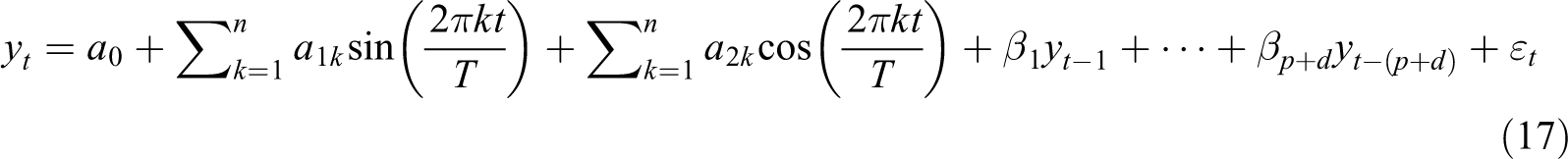
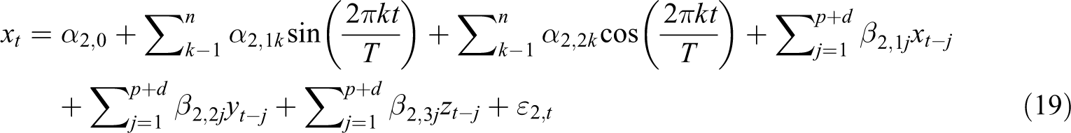
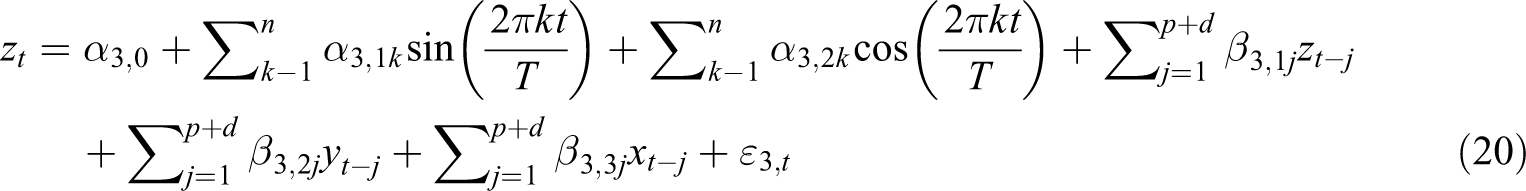
Overall, given the three variables employed in our study, y = GDPC, x = Tourism Development Index, and z = Financial Development Index, we can rewrite relationship (17) in its constituent parts as follows:

Under the Toda-Yamamoto specification, the null hypothesis of non-Granger-causality is based on zero restrictions on the first p parameters and the respective Wald statistic has an asymptotic χ2 distribution with p degrees of freedom. If the Wald statistic depends on k frequency, the solution is suggested in Becker et al. (2004) with the corresponding bootstrap distribution of the Wald statistic (Balcilar et al., 2010; Hatemi-J, 2002). We set the number of Fourier frequency to nmax and the number of lags to pmax and select the optimal of n and p that yields the smallest information criterion value (Akaike or Schawarz). Moreover, to test whether the trigonometric terms are significant, we carry out the F-test for the restriction
Results and discussion
To begin with our empirical analysis, we employ a battery of tests to diagnose the existence of cross-sectional dependence. Results from the three tests (Breusch–Pagan LM, by Breusch–Pagan (1980); Pesaran scaled LM, by Pesaran (2004); Pesaran LM, by Pesaran (2004)) have been displayed in the Online Appendix and reveal significant evidence of cross-sectional dependence (Online Appendix Tables 8 and 9). This situation of interdependence does not come to a surprise, because the economies of the various countries are quite interlinked in a highly globalized environment. Particularly, the tourism and the financial sectors are by definition, highly globalized and open to the rest of the world. With respect to tourism, which is the focus of this study, globalization occurs not only through travelling across the world and the opening of borders but also through the convergence of tourism preferences and ideals. The tourism market is becoming increasingly homogeneous (Vanhove, 2017) through its products and through its channels of marketing, logistics, and product development. The COVID-19 situation left aside, globalization in the aforementioned dimensions in tourism had been predicted to increase. For example, the United Nations World Tourism Organization had predicted an increase of long-haul travelling by 22% in 2030 (with 1995 as a reference year). Progress in technology and transport means and facilities also contribute to the globalization of tourism. Results from Online Tables 8 and 9, lead us to the employment of methodologies (at all steps of estimation) that take into account cross-sectional dependence. As far as unit root investigation is concerned, one such test is the CIPS test, namely the cross-sectional dependence adapted IPS unit root test presented in Online Appendix Table 9. Otherwise, various forms of bias will be introduced in the estimated results (Pesaran, 2006).
We continue the analysis with unit root testing, which reveals the existence of breaks dates, which are summarized in Figure 1 and have been sourced from Online Appendix Tables 11(a) to (c). Those tables have been placed in the Appendix of this article due to space considerations. These results are for unit roots with breaks by Im et al. (2003) and have been implemented in four versions: (i) Level shift with one break, (ii) level shift with two breaks, (iii) trend shift with one break, (iv) trend shift with two breaks.
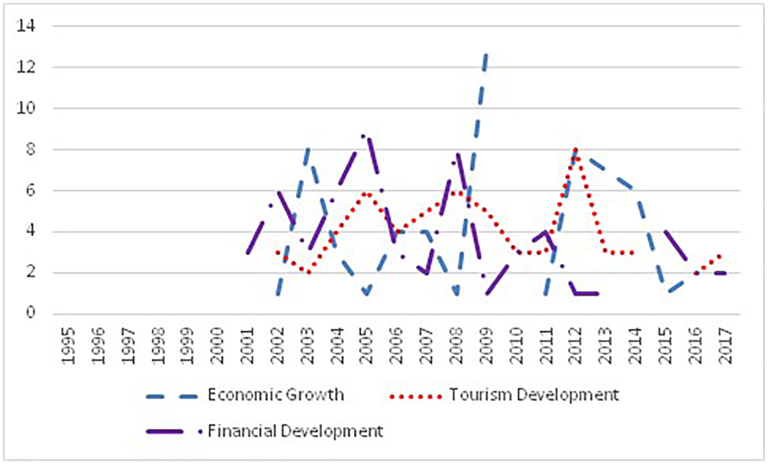
Number of breaks occurring in the period 1995–2017 for economic growth, tourism development, and financial development (based on results from Tables 11(a) to (c) in the Online Appendix).
Based on evidence from unit root tests, we observe that for all variables the breaks occur after the sixth year of the time span, both in the level and the trend version of the unit root equations. Our particular interest is for the time periods in which more than one breaks occur accumulatively across the unit root equations. More specifically, it can be easily observed that this is year 2009 for economic growth and year 2008 for the other two variables. Thus, the years 2008–2009 constitute a period which changes the way of integration in the variables. Another such point could be considered to be the year 2012 for the variable of economic growth and tourism development. Other break years that are common across variables are year 8 for economic growth and financial development, also the year 2005 for tourism and financial development.
It is worthy of observing that we have no structural breaks early in the studied period (which may be due to the use of 5% trimming), for example, from 1995 to 2000, although one would expect to see some effect from the Asian Financial Crisis or the Russian Financial Crisis in 1998 for Russia. In 2001, Turkey has abandoned the stabilization policy with respect to a stable exchange rate, in 2008 the Chinese currency rose, and these facts may cause some influence on the appearance of breaks (Dogan and Deger, 2018). The highest number of breaks in economic growth exist after the financial crisis of 2007, namely in 2009. Since this year gathers 13 occurrences of breaks, we can safely assume this is due to that financial crisis which was a very impactful fact through the income inequality that was caused to increase and the effects the crisis afflicted on productivity (OECD, 2020). The economic crisis has put much pressure on fiscal budgets. The years that follow in break occurrence, namely 2012–2014, signify an increase in growth for the countries which are revived and gradually recover from the crisis (Fullfact.org, 2018).
Generally, the structural breaks in the tourism and financial development follow more or less the evolution of breaks in the economic growth. In 2003, the UNWTO became a United Nations specialized agency and it is the leading international organization in almost every aspect of tourism, including tourism policy. In 2001 (11th September), the terrorist attack in the United States has transformed the tourism industry and it is that year that made policy makers in the United States realize the importance of that industry (Edgell et al., 2008). The period until 2007 was characterized by a period of growth, which was due to the development of information technology. Therefore, it is expected to experience structural breaks in all magnitudes, economic growth, tourism, and financial development, since all these figures are positively affected by the improvement in information technology (Jones, 2015).
These findings predispose us to the use of an estimator that will be robust and resilient to structural breaks. Next, we proceed with the investigation of cross-sectional dependence (Online Appendix Tables 8 and 9).
Cointegration
We have employed several cointegration tests to confirm cointegration in a robust way. Tables 2 to 5 display results from Westerlund (2007) panel cointegration test, Westerlund and Edgerton (2008) panel cointegration test with breaks, panel cointegration test with stochastic trends and the augmented mean group estimator (Eberhardt and Bond, 2009; Eberhardt and Teal, 2011) respectively. The tests have been applied in turn and progressively as we got evidence of no cointegration and tried additional tests. The null hypothesis of no cointegration has not been rejected in the first three tests (Tables 2 to 4). Only the augmented mean group estimator (Eberhardt and Bond, 2009; Eberhardt and Teal, 2010) has supported cointegation on the pooled data. Under the framework of this test, all coefficients represent averages across countries and the common dynamic process (c_d_p) is included as additional regressors, which accounts for common time-varying effect in all countries. The AMG was developed as an alternative to Pesaran (2006) Common Correlated Effects Mean Group estimator (CCEMG). It was introduced by Eberhardt and Bond (2009) and developed by Eberhardt and Teal (2010). It is carried out as follows: (i) A pooled regression model augmented with year dummies is estimated by first difference OLS and the coefficients on the (differenced) year dummies are collected. This is the c_d_p. (ii) The group-specific regression model is then augmented with this process. (iii) Like in the MG and CCEMG, the group-specific model parameters are averaged across the panel (Bond and Eberhardt, 2003). ΔDt represents the year dummies, while the panel dynamic process is represented by ct in equation (21).
Westerlund (2007) panel cointegration test.
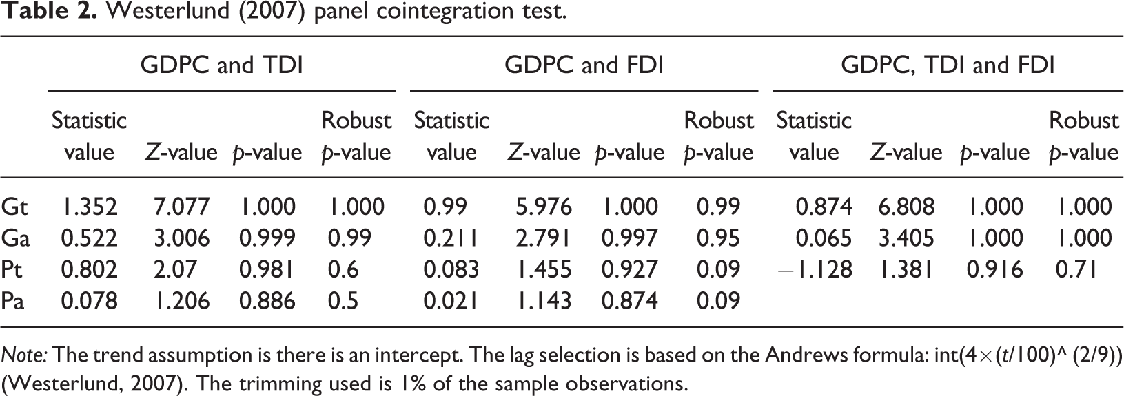
Note: The trend assumption is there is an intercept. The lag selection is based on the Andrews formula: int(4×(t/100)^ (2/9)) (Westerlund, 2007). The trimming used is 1% of the sample observations.
Westerlund and Edgerton (2008) panel cointegration test with breaks.
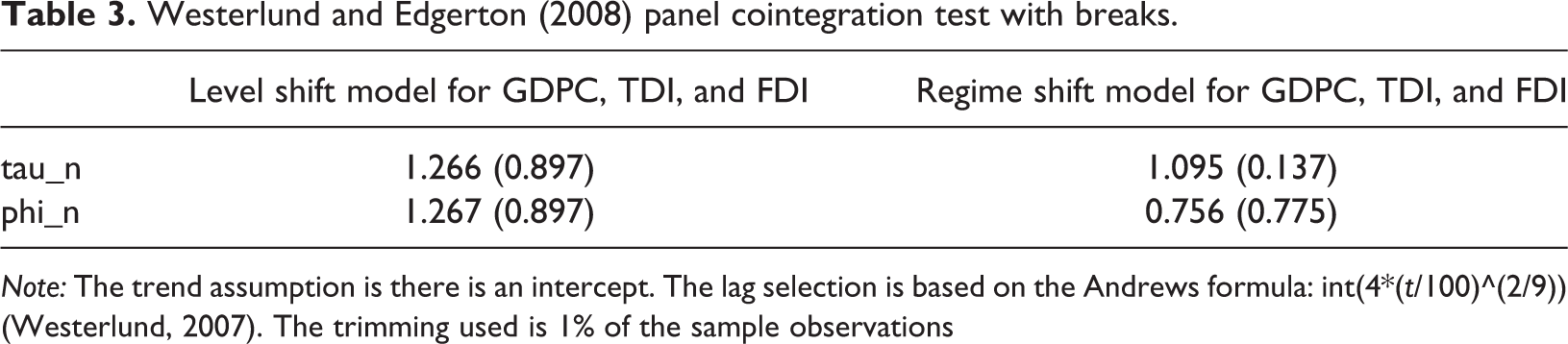
Note: The trend assumption is there is an intercept. The lag selection is based on the Andrews formula: int(4*(t/100)^(2/9)) (Westerlund, 2007). The trimming used is 1% of the sample observations
Panel cointegration with latent factors (Bai et al., 2009).
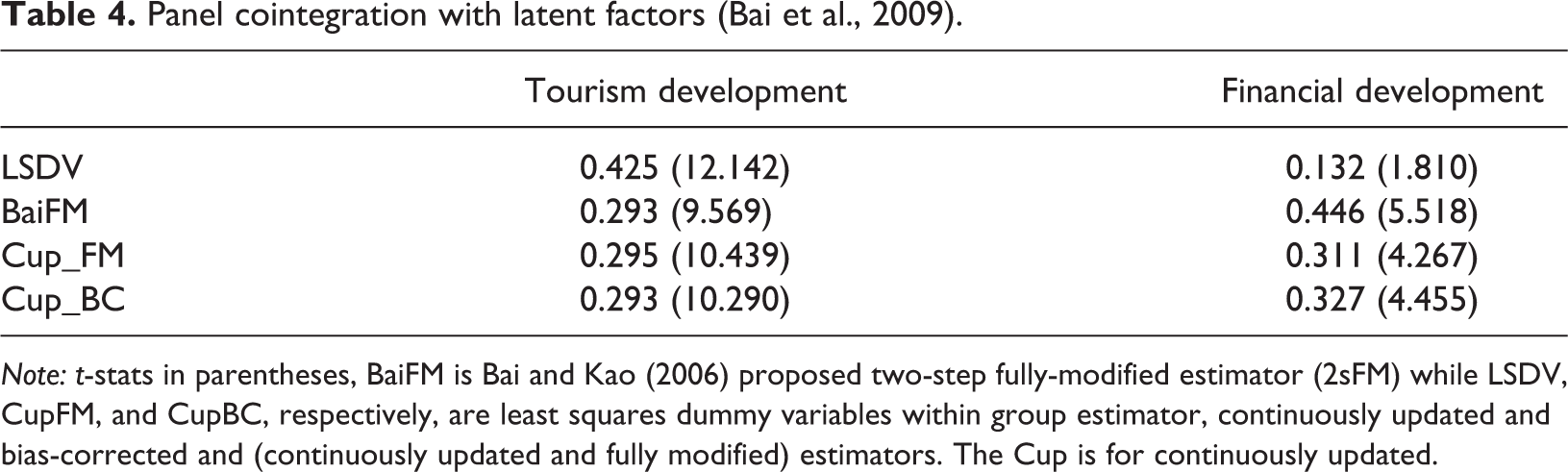
Note: t-stats in parentheses, BaiFM is Bai and Kao (2006) proposed two-step fully-modified estimator (2sFM) while LSDV, CupFM, and CupBC, respectively, are least squares dummy variables within group estimator, continuously updated and bias-corrected and (continuously updated and fully modified) estimators. The Cup is for continuously updated.
Long-run relationships with an augmented mean group estimator (Eberhardt and Bond, 2009; Eberhardt and Teal, 2010).
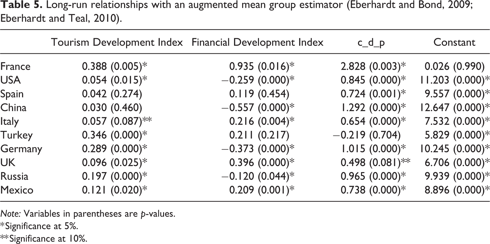
Note: Variables in parentheses are p-values.
* Significance at 5%.
** Significance at 10%.

This method accounts for cross-sectional dependence and non-stationarity and heterogeneous slope coefficients across countries. It eliminates the asymptotical bias in the estimators due to the endogeneity of the regressors (Pesaran, 2015).
Based on the results from AMG (Table 5), tourism development has a positive sign in all countries revealing that there is a long-run positive relationship between tourism and economic growth. Only in two countries is the relationship insignificant: Spain and China. As far as the financial development is concerned, it appears to have a positive relationship with economic growth in the following four countries: France, Italy, the United Kingdom, and Mexico. A significant negative relationship is noted for the United States, China, Germany, and Russia. The c_d_p is significant in all countries except for Turkey, while the constant is also significant in all countries except for France, since the c_d_p variable captures the time-invariant fixed effects and has been generated from the dummies. Considering the elasticities of tourism development with respect to economic growth, the highest elasticities are observed for Turkey (3.46%) and France (3.88%), while the lowest are observed for the United States (0.54%) and the United Kingdom (0.96%. Considering the elasticities of financial development with respect to economic growth, the highest is in France (+9.35%) and the United Kingdom (+9.96%) and the lowest in Russia (−1.20%) and Mexico (+2.09%).
Table 4 presents the results assuming a framework of data, which are non-stationary, or some of them are stationary and the structural errors e it are characterized by cross-sectional dependence and non-stationarity and possibly correlated with the explanatory variables. In the new tests shown here, e it is assumed to have a common component and a stationary idiosyncratic component. The latent e it can be decomposed into a worldwide component Ft and a country-specific component u it .

with Ft being an r×1 vector of latent common factors, λi is an r×1 vector of factor loadings, and u it is an idiosyncratic error. Assuming that Ft is the source of non-stationarity leads to a model with latent common trends, the problem is dealt with the treatment of the common I(1) variables as parameters. These are estimated jointly with the beta coefficients in an iterated procedure. To handle the problem of bias from endogeneity and serial correlation, two new estimators have been constructed (the CupBC and the CupFM) by Bai et al., (2009). The two estimators are called Cup because they are continuously updated. CupBC estimates the asymptotic bias directly. CupFM makes such modifications that the limiting distribution does not depend on nuisance parameters.
The Bai FM is a two stage fully modified test, which is the CupFM estimator with one iteration and is a less efficient estimator than the CupBC and the CupFM. Initially, Bai and Kao (2006) had developed a fully modified two-step estimator (BaiFM). The BaiFM treated the I(0) common shocks as part of the error process. This estimator is linear and can be obtained when Ft is observed.
Based on results from Table 3, we see that the results from the five statistics do not diverge and the same results are reached in terms of cointegration. While financial development has a t-value less than 2 under the LSDV framework, this is rectified in the rest of the tests which also correct for the aforementioned bias. Overall, cointegration is confirmed in this framework with global stochastic trends and it is good that we have investigated cointegration under these settings, because the Westerlund tests would have produced spurious results with the underlying generating parameter we have at hand.
Granger-causality
We start the investigation of Granger-causality with Dumitrescu and Hurlin (2012) panel Granger-causality test (hereafter DH), which is one of the most popular Granger-causality tests in the panel data literature. This test relies on testing the following two hypotheses (equations (23) to (24)).


The approach resembles that of Im et al. (2003) for panel unit roots. The DH test is the extension of the Granger-causality test to cross-sectional dependence and serial correlation.
Dumitrescu–Hurlin method is only a bivariate method and does not consider a mixed order of integration. Foremost, it doesn’t consider structural changes, and this is the reason that after we apply this method, we compare the obtained results with the rest of the methods we have used.
The results presented in this section are in essence multivariate VAR model estimations and the variables we are using are endogenous variables. Therefore, the presentation of various model configurations serves to prove the robustness of our reached results. As will become obvious with the results presented in the following tables, the Fourier approximated results are more eloquent and reveal relationships that would otherwise remain overshadowed. This means that the tourism-growth markets in the sampled countries have experienced structural transformations that are worthy of pinpointing and analyzing. There are different transmission channels between tourism and the financial sector with respect to their impact in economies. Understandably, both the tourism and finance are quite interrelated to the level of income generated in the countries we are studying. This article deals with 10 countries that have been employed as the 10 top tourist destinations in Shahzad et al. (2017). For all these countries, a positive relationship between tourism and economic growth is documented, although for some of these countries such as China and Germany the relationship has been found to be weaker, possibly because of the higher economic importance of other sectors in those economies. Foremost, other countries such as the United States, the United Kingdom, Mexico, Turkey, and Spain present a positive relationship between the two magnitudes, but the relationship becomes stronger in periods of economic recession in those countries. This means that these countries use tourism as a shelter in bad economic times.
Based on results from Table 6, we observe unidirectional Granger-causality from tourism development to economic growth in five out of the ten countries in our sample. These are the United States, Spain, Italy, the United Kingdom, and Mexico. In four out of the five countries in which the TLGH is supported, there is also support of the finance-led growth hypothesis. Therefore, the finance-led growth hypothesis is also confirmed in the United States, Spain, the United Kingdom, and Mexico, while this is also supported for France where no support for the tourism-led hypothesis is noted. Last, we observe that both magnitudes such as tourism and financial development Granger-cause economic growth in five countries again. These are the same five ones in which the finance-led growth hypothesis is confirmed. Thus, only in Italy is the TLGH confirmed with no respective effect from the side of the financial sector alone or its interaction term with tourism.
The panel Granger-causality results based on Emirmahmutoglu and Kose (2011).
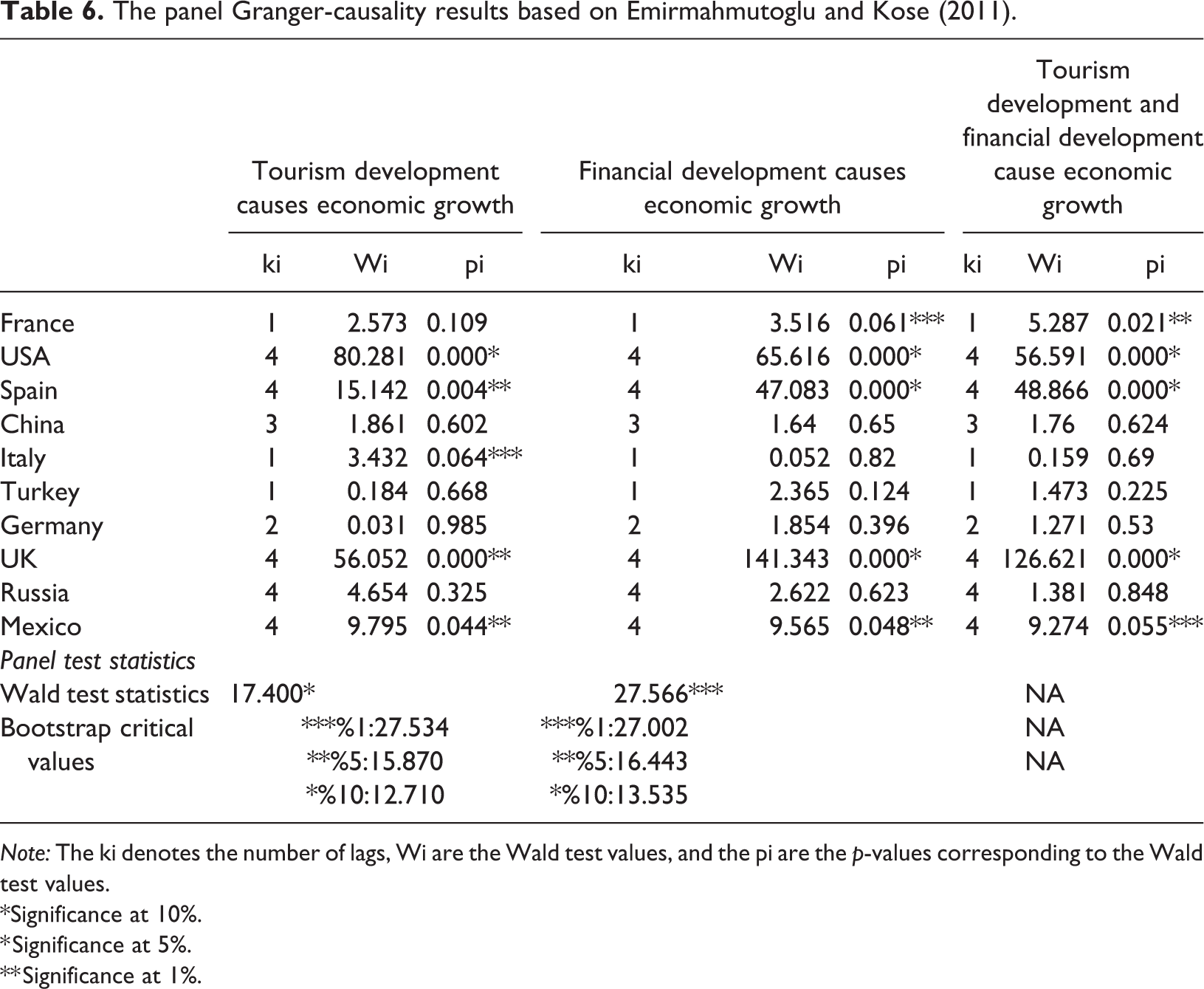
Note: The ki denotes the number of lags, Wi are the Wald test values, and the pi are the p-values corresponding to the Wald test values.
*Significance at 10%.
* Significance at 5%.
** Significance at 1%.
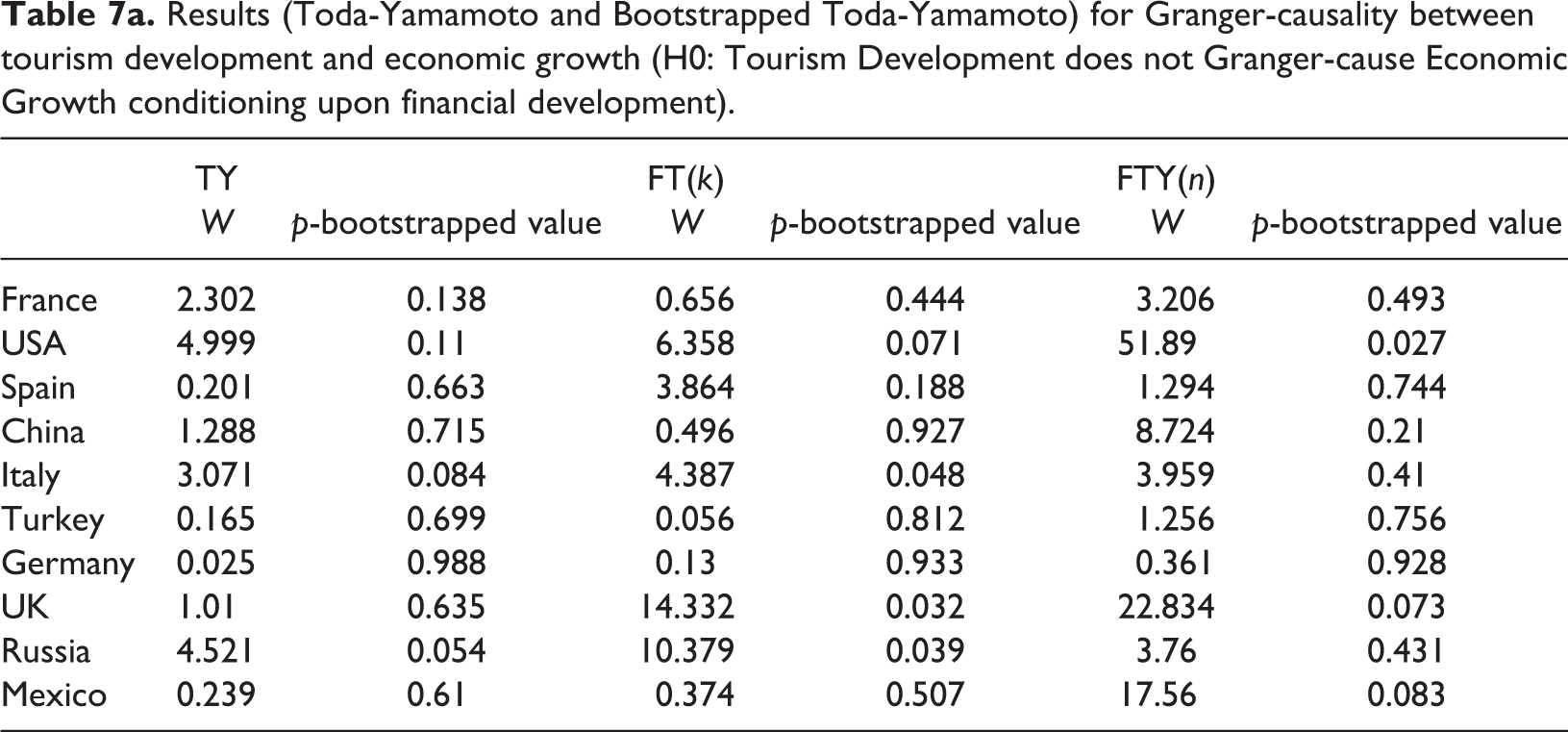
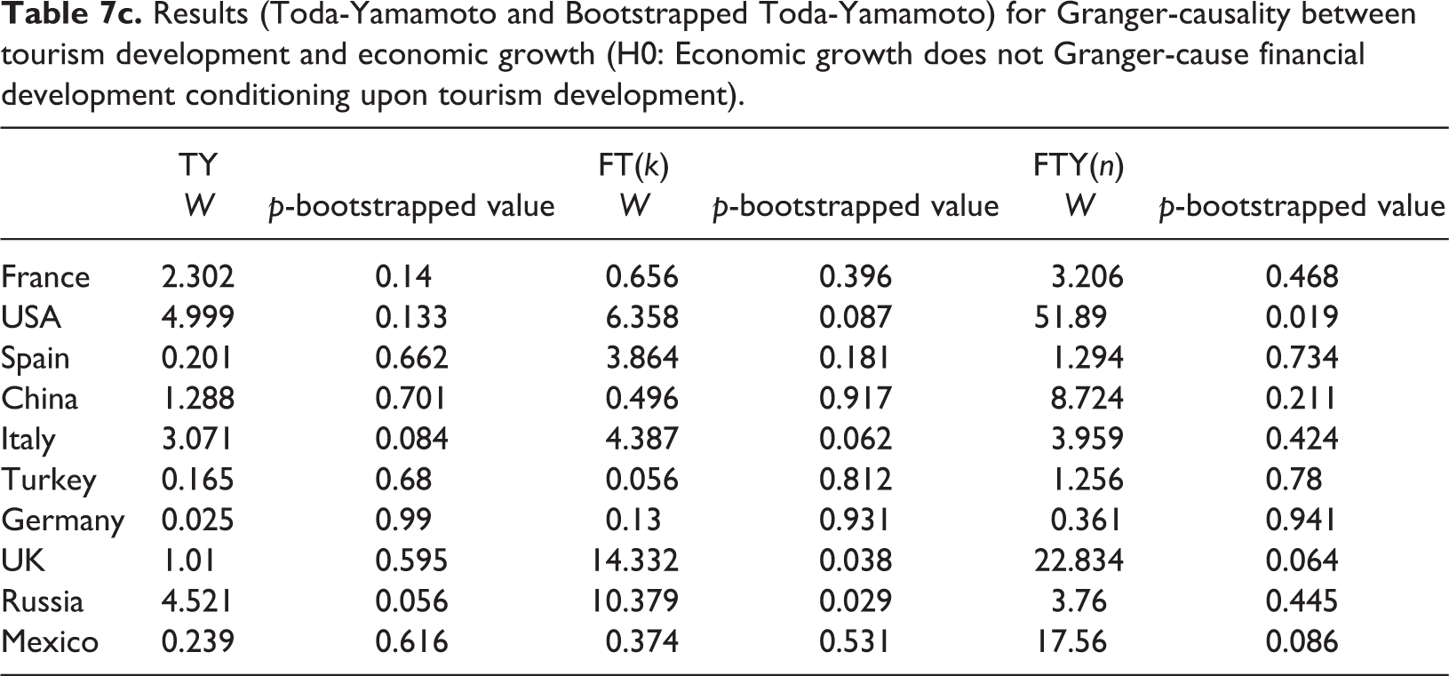
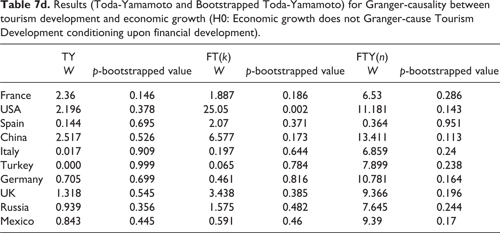
Results presented in Table 7(a) to (d) are obtained following the estimation method of Durusu-Ciftci et al. (2020). Each table presents three tests, namely TY which is the Toda and Yamamoto (1995) test, FT(k) is the Wald test for Fourier frequency, and FTY(n) is Fourier version of Toda and Yamamoto test which is proposed by Durusu-Ciftci et al. (2020).
Results (Toda-Yamamoto and Bootstrapped Toda-Yamamoto) for Granger-causality between tourism development and economic growth (H0: Tourism Development does not Granger-cause Economic Growth conditioning upon financial development).
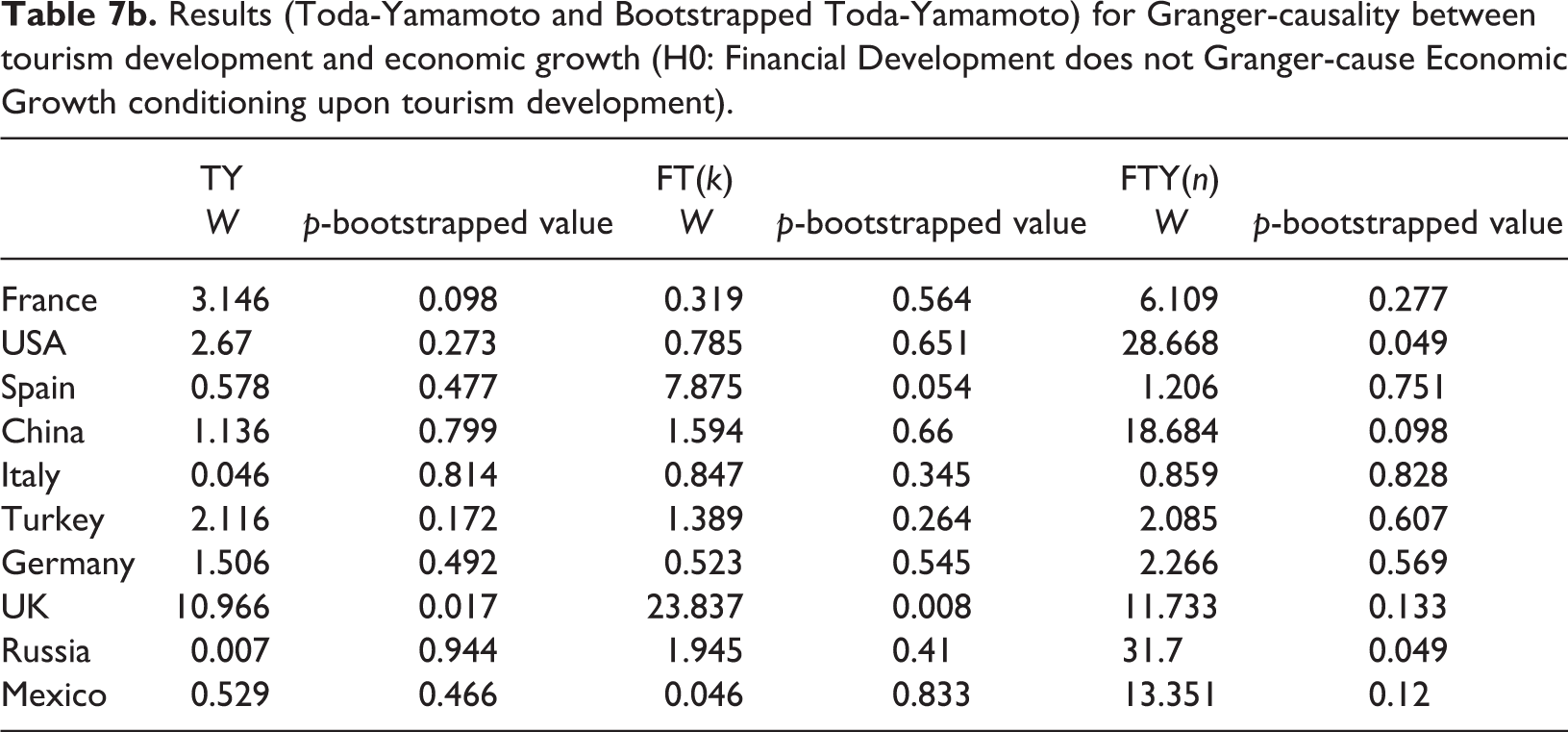
Results (Toda-Yamamoto and Bootstrapped Toda-Yamamoto) for Granger-causality between tourism development and economic growth (H0: Financial Development does not Granger-cause Economic Growth conditioning upon tourism development).
Results (Toda-Yamamoto and Bootstrapped Toda-Yamamoto) for Granger-causality between tourism development and economic growth (H0: Economic growth does not Granger-cause financial development conditioning upon tourism development).
Results (Toda-Yamamoto and Bootstrapped Toda-Yamamoto) for Granger-causality between tourism development and economic growth (H0: Economic growth does not Granger-cause Tourism Development conditioning upon financial development).
Before presenting and commenting on the findings about the channels of interaction among the economy, tourism, and the financial sector, it is important to underline that the evidence on direction of Granger-causality are country specific (Sokhanvar et al., 2018). First, this relationship depends on how many of the tourism inputs are imported or produced within the country of tourism production. If most of those inputs are imported, this entails a smaller multiplier effect from tourism. In some countries, tourism growth occurs with no respect and consideration for the environment or the locals. Higher number of tourists may lead to increase in the prices, which in turn decrease domestic demand and welfare. The investment and growth in other sectors is higher than in the tourism sector and this overshadows tourism. Higher economic growth may provide better opportunities for investment in the tourism industry, and this will increase tourism. That being said, one can easily understand that the discussion of results has to be country specific too and this is what we do in the following paragraphs based on the findings we receive from Tables 7(a) to (d).
Table 7(a) reports Granger-causality between tourism development and economic growth. Initially, with the conventional Toda-Yamamoto estimation, we observe this Granger-causal relationship only for Italy and Russia. When the Fourier approximation is in place, richer results are produced and the United States, the United Kingdom and Mexico are also noted for the impact their economic growth absorbs from tourism. In the United States, a Granger-causal link stemming from tourism development is widely known (Isik et al., 2018) and expected. In the United Kingdom, the tourism sector is growing much faster than other sectors such as manufacturing, construction, and retail (VisitBritain, 2020). Actually, the tourism sector is contributing higher than the banking sector, namely 11% versus 6.1% of GDP (Barlow, 2019). In Mexico, despite the tourism sector recovering quickly to its precrisis GDP levels and the H1N1 flu outbreak of 2009 (OECD, 2017), the sector needs a better transport system and better lending opportunities for microenterprises.
In Russia, tourism is of ascending importance for the economic development of the country (Lavrova and Plotnikov, 2018) and there is a variety of reasons why this is happening (natural parks with rich natural potential, cultural, and historic heritage, infrastructure and the perceived safety as well as neighborhood with a vast number of populous Asian countries with rising incomes). Until 2003, the country had more arrivals than departures. Russia is a transition economy with new and continuous development in tourism from a policy point of view. However, the economic crisis and the depreciation of the ruble (2015–2015) as well as the geopolitical problems with countries such as Turkey, Georgia, and Ukraine, increase the uncertainty faced in tourism. Generally, as will be obvious with the rest of the tables, significant results are not a surprise because we have a sample of the 10 top tourist destinations. However, the value of our results lies in the sparsely corroborated significance of the results (contrary to Shahzad et al. 2017), which may constitute evidence of tourism saturation for countries which do not appear as significant.
To continue with the presentation of results, Table 7(b) reports Granger-causality results between financial development and economic growth. Thus, the Toda-Yamamoto test reveals Granger-causality running from financial development to economic growth for France and the United Kingdom. When breaks are inserted in the analysis through the Fourier approximations, we get that the finance led growth hypothesis is supported in Spain and still in the United Kingdom, but not in France. Apparently, as far as the finance-led growth hypothesis is concerned, our data provide stable and coherent support only for the United Kingdom, which undoubtedly is a business and finance hub. However, the F-test is not significant for the Fourier approximation and thus there is no support for smooth structural breaks that characterize the finance-led growth hypothesis in this country. Particularly for Spain, the Comprehensive National Tourism Plan (2012–2015) has focused on the reduction of seasonality through new investments and marketing opportunities (Gutiérrez-Domènech, 2014). It is important to stimulate alternative tourism products in addition to beach tourism (Hidalgo and Maene, 2017). Moreover, the United Kingdom, Germany, and France are the principal countries of origin for international tourists visiting Spain. Therefore, the economics of those countries affect tourism entrants in Spain.
Table 7(c) presents the results for Granger-causality between economic growth and financial development. Based on results from Toda-Yamamoto, we see that this form of unidirectional Granger-causality is very weakly supported and only for two countries, Italy and Russia. Compared with the Fourier counterpart of TY, this Granger-causality direction is supported in double the number of countries than it was supported in the simple TY. These countries are the United States, Italy, the United Kingdom, and Russia. The Fisher test though confirms significance only for two of them, namely the United States and the United Kingdom. As far as Italy is concerned, there is a bidirectional Granger-causality between market diversification and economic growth (Can and Gozgor, 2018). In this country, tourism receives support from the Culture and Innovation 2014–2020 program financed by European Union Structural Funds (OECD, 2018). Regarding Russia, a lack of affordable long-term debt instruments to investors is widely acknowledged despite the potential provided by poorly developed tourism facilities, which are an obstacle for the attraction of private investment (Maloletko et al., 2015).
Based on Table 7(d), the hypothesis that economic growth does not Granger-cause tourism is rejected only in the United States and within the Fourier approximated TY. Thus, we have very little evidence that economic growth Granger-causes tourism development. Therefore, under no circumstances could we speak of a feedback relationship in the tourism-growth relationship in these countries. Maybe, that could be supported only for the United States. Particularly for the United States, we should note that it has issued the Travel Promotion Act of 2009 (TPA) and the Travel Promotion, Enhancement and Modernization Act of 2014 (HR 4450). The former has established a public–private partnership in tourism business as “Brand USA.” This Act enhances the distribution of information on the US entry policies and promotes tourism within the United States. Under the Travel Promotion Act, Brand USA is enabled to access up to $100 million in federal matching funds to perform its duties based on a one-to-one ratio of public to private funds. The latter reauthorized and amended the Travel Promotion Act of 2009 through September 30, 2020, and describes the procedures between the Department of Commerce and the Corporation for Travel Promotion (Brand USA). The Travel Promotion Fund cap remains set at US$100 million in federal matching funds.
Overall, the results of this article enrich the results of the study by Shahzad et al. (2017) because without contradicting them, they augment that study and throw light to the direction of Granger-causality. That is also done in a more robust way, after making allowance for structural breaks. This result of no support for the growth-led tourism hypothesis is not a surprise because all the countries hosted in our sample are high-income or middle-income countries and this means they already have reached a level of economic development that has been built by a variety of economic activities and they are not exclusively reliant on tourism. The growth-led tourism hypothesis postulates that while resources become available for tourism, they create a positive business climate that encourages proliferation of this positivity to other economic sectors that can flourish as well. However, this is unlikely to happen in cases where the economies also rely on other vibrant sectors. This is the case with all the economies we have in our sample. Although they are top tourist destinations, they also have important non-tourism industries. With all this, it is meant to suggest that it is easier to observe the growth-led tourism hypothesis in small island countries that have developed tourism as a single industry.
Results from Table 7(a) to (d) present Granger-causality between tourism development and economic growth as well as financial development and economic growth. The VAR estimations are from Toda-Yamamoto (TY) and FTY frameworks. Juxtaposing the two sets of results in each of these tables, we observe that the Fourier approximated Toda-Yamamoto provides more accurate results with Granger-causality in the sampled countries. Thus, while TY reveals support of the TLGH only in two countries, namely Italy and Russia, when structural breaks are taken into account, more countries appear to be significant in their bidirectional relationship running from tourism to economic growth. Therefore, the TLGH is supported for the United States, Italy, the United Kingdom, and Russia. Had we ignored the existence of breaks, we would have considered only Italy and Russia in this matter. This finding is aligned more with existent tourism–growth literature findings (Brida and Pulina, 2010). Besides, the United States and Italy are among the most visited outbound destinations and tourism contributes significantly in their economic growth through various channels. Tourism entails a high inflow of foreign currency, thus is a foreign exchange contributor, which in turn can buy for countries additional capital for their production. In addition to that, tourism stimulates investment to new capital infrastructure, human capital and competition (Brida and Pulina, 2010), employment increase, and the diffusion of new technologies. Not to be ignored for their contribution to the wider economy are the induced effects from tourism as well as the indirect effects. The TLGH has been confirmed, in the past, for Italy by Cortés-Jiménez and Pulina (2010). Russia and the United Kingdom have not received much attention in the past with respect to the validation of the TLGH and thus this research contributes to the solution of gauging the literature gap in these countries. The United Kingdom is more regarded as a business and education destination rather than a tourism destination, while Russia is certainly not a popular tourism destination, but based on our findings, this country’s economic growth is significantly benefited from tourism. However, the study by Shahzad et al., (2016) also includes Russia and the United Kingdom and finds support of the TLGH and notes that for countries where variations exist in support of the TLGH is because these countries have other dynamic sectors in their economies which contribute to their growth in a more decisive and dynamic way.
Our results are partly in line with previous literature. For example, as far as Mexico is concerned, Dritsakis (2012) and Eugenio-Martin et al., (2004) have found that tourism has a larger positive Granger-causal contribution in smaller and developing countries. Particularly, based on the results from Eugenio-Martin et al., (2004), tourism has not helped much the countries of Latin America in their economic development. A similar result was reached by De Vita and Kyaw (2016). Katircioglu (2009) also has not found support for the tourism–growth hypothesis in Turkey. The results are also formed by the stage of the life cycle of various destinations within the countries. For example, Brida and Giuliani (2013) have not found support for the TLGD for Tirol in Germany. Based on Surugiu and Surugiu (2013) and Tugcu (2014), each destination has its intrinsic characteristics, political, economic, financial, sociological, and environmental peculiarities that affect the tourism effect transmission channel into the economy and vice versa. As far as Italy and Spain are concerned, Proença and Soukiazis (2008) have found support for the TLGH. Particularly, they find that 1% increase of tourist revenue causes an increase by 0.026% in the GDP per capita in four Mediterranean countries. Dritsakis (2012) in his study for France, Italy, Spain, and Turkey has estimated an elasticity equal to 1.24.
There is doubt about whether tourism can be a vehicle for the economic growth of rich countries (Smeral, 2001). This is so because in developed economies, tourism interacts with the other sectors. Due to the phenomenon of Baumol disease, the lower productivity in tourism compared to the other sectors of the developed economies cannot be accompanied by lower wages. Tourism is a labor-intensive industry, and it is not easy to reduce labor costs. Thus, tourism prices are increased (Croes and Rivera, 2016) to gauge the gap. Thus, to facilitate economic growth from tourism, a reliable forecasting should be used by policy makers. Results from studies such as ours combined with computable general equilibrium models (Dwyer et al., 2003) could contribute to the implementation of policies that will make tourism an engine for economic growth, even in rich countries. All the results of the paper (cointegration and Granger-causality) have been included in Table 12 in the Online Appendix.
Conclusion
In many countries of the world, inbound tourism plays an important role for economic growth, because tourism is an important part of their exports. In the last two decades, the tourism-growth nexus has developed and since then, it has been continuously studied by many scholars who reach different results based on the countries they study, the data and the methods they employ, thereby urging the need of studying the field more rigorously and with more sophisticated methods. Tourism entails economic and technological spillovers, improves the efficiency of the economies, because it contributes to the efficiency of resources and the increase in their total productivity. Labor staff becomes more specialized, better management practices are learned, and more efficient forms of organization are transferred to the economies together with an improvement in competition. This formulates the so-called TLGH. On the other hand, the achieved economic growth in one country may appear to affect tourism development, through the investment on capital infrastructure and the buys in intermediary goods. The knowledge of the direction of Granger-causality between tourism and economic growth is very important, because policy makers will acquire good knowledge of how and which sectors to allocate public revenue to increase the citizen income or invest in tourism infrastructure (airports, accommodation, etc.). Of course, there may be countries in which economic growth has not been Granger-caused by tourism, because these countries have relied on other sectors to increase their total economic growth.
The current study examines the Granger-causal links between tourism development, financial development, and economic growth for the period 1995–2015 in the top 10 tourism destinations. Since these countries have been subject to either smooth or structural changed transitions in the above magnitudes for the studied period, we employ the FTY method after a series of other methods, which prove the robustness and stability of the channels of interaction among these crucial magnitudes. It appears that structural shifts are not to be neglected, because they generate more concrete evidence about the TLGH. Nowadays as tourism is a global phenomenon, all countries participate into it to a higher or a lower degree. Unless we employ a highly sophisticated method such as this, we may receive obscure results that overestimate or underestimate the Granger-causal importance of tourism in an economy and thus mislead policy makers to devote the scarce public funds into uses that would not be of priority for an economy. The dependence of tourism development on the financial development should not be overseen because in order for tourism to make sound policy decisions, the financial system of a country must be available and able to contribute towards this expansion and development.
As a note for further research, that should be directed into reaching tourism and financial data for a larger number of countries, so that policy makers observe the new tourism destinations that become established year by year. Also, repeating this study in the future with longer series of data, as they become enriched year by year, would be important to observe whether the currently observed relationships pertain or some of the top tourism destinations become outdated and saturated. It is important to realize that the sparse corroboration of the tourism-growth significance in the top 10 tourism destination may signify the formation of a saturation point for those countries and the need for action to expand their life cycle as existent products or their diversification to the consumers’ eyes to offer and signify different experiences to potential tourists. Overall, the FTY Granger-causality framework has highlighted only very few countries supporting the tourism-growth hypothesis compared to other studies. Last, since tourism can be measured in terms relative to the size of the economy, the top 10 ranking countries may defer. This entails that countries such as China may disappear off the ranking in favor of small countries such as Barbados, for instance. As an idea for further research, it would be relevant to test the current methodology is such small countries.
Supplemental material
Supplemental Material, sj-docx-1-teu-10.1177_13548166211021174 - The stability of interaction channels between tourism and financial development in 10 top tourism destinations: Evidence from a Fourier Toda-Yamamoto estimator
Supplemental Material, sj-docx-1-teu-10.1177_13548166211021174 for The stability of interaction channels between tourism and financial development in 10 top tourism destinations: Evidence from a Fourier Toda-Yamamoto estimator by Angeliki N Menegaki and Aviral Kumar Tiwari in Tourism Economics
Footnotes
Acknowledgment
The authors would like to thank two anonymous reviewers and the editor for their valuable suggestions for the improvement of this article.
Declaration of conflicting interests
The author(s) declared no potential conflicts of interest with respect to the research, authorship, and/or publication of this article.
Funding
The author(s) received no financial support for the research, authorship, and/or publication of this article.
Note
Supplemental material
Supplemental material for this article is available online.
References
Supplementary Material
Please find the following supplemental material available below.
For Open Access articles published under a Creative Commons License, all supplemental material carries the same license as the article it is associated with.
For non-Open Access articles published, all supplemental material carries a non-exclusive license, and permission requests for re-use of supplemental material or any part of supplemental material shall be sent directly to the copyright owner as specified in the copyright notice associated with the article.