
Abstract
The availability of tourism-related big data increases the potential to improve the accuracy of tourism demand forecasting but presents significant challenges for forecasting, including curse of dimensionality and high model complexity. A novel bagging-based multivariate ensemble deep learning approach integrating stacked autoencoder and kernel-based extreme learning machine (B-SAKE) is proposed to address these challenges in this study. By using historical tourist arrival data, economic variable data, and search intensity index (SII) data, we forecast tourist arrivals in Beijing from four countries. The consistent results of multiple schemes suggest that our proposed B-SAKE approach outperforms the benchmark models in terms of level accuracy, directional accuracy, and even statistical significance. Both bagging and stacked autoencoder can effectively alleviate the challenges brought by tourism big data and improve the forecasting performance of the models. The ensemble deep learning model we propose contributes to tourism demand forecasting literature and benefits relevant government officials and tourism practitioners.
Keywords
Introduction
Tourism demand forecasting plays a crucial role in tourism management. On the one hand, tourism resource planning based on accurate demand forecasting is of great significance for avoiding unnecessary losses, due to the perishability of tourism products (Chu, 2011; Law et al., 2019; Shen et al., 2008). On the other hand, tourism demand forecasting can effectively help the government and tourism practitioners guide tourists properly, and thus improve the service quality and tourists’ experience (Liu et al., 2018; Zhang, Wang, et al., 2020).
Tourist demand forecasting approaches, used by the majority of quantitative studies, include various time series, econometrics, artificial intelligence (AI) approaches, and the combinations of these approaches (Jiao and Chen, 2018; Song et al., 2019; Song and Li, 2008). AI approaches can not only effectively capture the nonlinear characteristics between variables but also require little specialized expertise as data-driven approaches. Therefore, more and more researchers develop various powerful AI approaches to further advance the literature of tourism demand forecasting (Song et al., 2019; Zhang, Wang, et al., 2020). Notably, deep learning has been the research hot spot in this field recently (Law et al., 2019; Lv et al., 2018; Zhang, Li, et al., 2020, 2021).
The availability of tourism big data is improving gradually. In addition to historical tourist arrival data, the data widely used in current tourism demand forecasting literature mainly include economic variable data and search intensity index (SII) data. The causal econometric approaches have revealed the most crucial economic variables that determine the demand for international tourism. Specifically, these economic variables are summarized by Athanasopoulos et al. (2017), including tourism prices in a destination relative to those in the origin country, tourism prices in competing destinations, tourists’ income, and exchange rates. Additionally, with the booming in web search technology, tourists seek travel information by using search engines before traveling. These search behaviors are statistically generated into SII data that could be used to accurately measure tourists’ attention (Bangwayo-Skeete and Skeete, 2015; Fesenmaier et al., 2010). A set of effective methods for key word selection and data aggregation to form the indicator has been gradually developed (Li et al., 2017; Yang et al., 2015). The application techniques of SII data have been preliminarily established.
According to the concept of “data-intensive forecasting” proposed by Bunn (1989), a way to further improve forecast accuracy is by making use of the availability of multiple information and computing resources. Analogously, Song et al. (2013) point out that combining forecasts considering different data has become one of the most important and effective ways to improve forecasting performance. Inspired by this modeling idea, this study incorporates historical tourist arrival data, economic variable data, and SII data mentioned above into the forecasting framework. Nevertheless, introducing large amounts of data also poses huge challenges for forecasting. First, tourism-related big data means many influential factors potentially affecting tourism demand. With the increase of potential features, sample data will become sparse in the feature space, which eventually leads to curse of dimensionality and affects the forecasting effect (Law et al., 2019). Second, the data with many explanatory variables also increase the complexity of the model, resulting in large variance and overfitting (Zhang, Li, et al., 2020, 2021). Feature engineering is an effective way to solve the above two problems, but traditional feature extraction requires a lot of expert knowledge and manual work (Law et al., 2019; Lv et al., 2018).
To address these challenges, a bagging-based multivariate ensemble deep learning model, integrating stacked autoencoder and kernel-based extreme learning machine (B-SAKE) is proposed for tourism demand forecasting. Concretely, the deep learning technique automatically extracts mining features by simulating the brain’s pattern to process information and does not require much domain knowledge and human resource (Pouyanfar et al., 2018). Researchers have examined unsupervised feature learning applied in tourism demand forecasting. For example, Li et al. (2018) utilize principal component analysis (PCA) to reduce the dimension of data features, thus effectively reducing the redundant information of data. Stacked autoencoder (SAE) is capable of learning nonlinear relationships, which could be regarded as a more powerful nonlinear generalization of PCA. Bagging generates multiple data sets for training a set of models to improve the stability of forecasting and reduce variance effectively (Athanasopoulos et al., 2017; Inoue and Kilian, 2008) and its powerful performance has been demonstrated in many forecasting fields. Kernel-based extreme learning machine (KELM) has not only high computational efficiency but also better forecasting performance than extreme learning machine (ELM) because the random map in ELM is replaced by the kernel in KELM (Sun et al., 2019).
We conduct numerical experiments for Beijing international tourist arrivals. To verify the effectiveness of the models, we consider the cases of tourist arrivals in Beijing city from four origin countries including the United States, the United Kingdom, Germany, and France. In addition to its 67% market share in the United States, Google has more than 90% of the search market in the other three countries. SII data are more representative in these countries, and other data required in the models are publicly available. The results of the empirical study are fourfold: (1) Both bagging and SAE can improve the forecasting performance of the models. (2) Our proposed B-SAKE model is the most accurate in different forecasting schemes (i.e. one-step-ahead vs. multistep-ahead, and in-sample vs. out-of-sample) regarding the performance evaluation criteria including mean absolute percentage error (MAPE), normalized root mean square error (NRMSE), and directional symmetry (DS). (3) This forecasting model performs better than other benchmark models from the statistical perspective (Diebold-Mariano test and Pesaran-Timmermann test). (4) The consistency of our findings across the four countries we considered is encouraging.
The objective of this study is to propose a novel ensemble deep learning model to mitigate the curse of dimensionality and high model complexity caused by tourism big data and verify its good forecasting accuracy and stability. The most relevant literature is Zhang, Li, et al. (2021), who also points out that there may be overfitting problems in the deep learning model. They increase the data volume available for training through the decomposition method and improve the efficiency of feature extraction by designing a duo attention layer. Correspondingly, in the ensemble model we develop, bagging and SAE are responsible for implementing similar functions. Given excellent forecasting performance and consistency in multiple forecasting cases, our proposed B-SAKE model contributes to tourism demand forecasting literature and benefits relevant government officials and tourism practitioners.
The rest of this study is organized as follows. The second section details the literature on tourism demand forecasting with SII data and tourism demand forecasting with deep learning. The third section introduces related methods and describes the conceptual framework of this study. The fourth section provides a case study on Beijing tourist arrivals and compares the results of our proposed B-SAKE model with those of benchmark models. Finally, conclusions and limitations are summarized in the fifth section.
Literature review
Tourism demand forecasting with SII data
Search engines can provide a time series index of the volume of queries users using the search engine in a specific geographic area (Choi and Varian, 2012; Padhi and Pati, 2017), which is referred to in the literature as SII data. Social psychologists outline the spatiotemporal frequency of specific search terms provided by web search engines can reflect the attention of specific user groups on this issue in a specific time space (Lai et al., 2017). In terms of tourism, travelers seek relevant information through search engines regarding almost all aspects of the trip, including accommodations, transportation, attractions, and dining (Fesenmaier et al., 2010; Yang et al., 2015). Therefore, SII data, as a measure of tourists’ attention, have been widely used in tourism demand forecasting literature (Tang et al., 2020).
Choi and Varian (2012) first introduce Google Trends data to forecast visitor arrivals in Hong Kong, and the positive effect of Google Trends data in forecasting is demonstrated by using visitor arrival data from nine origin countries. However, they only consider the Google Trends index for “Vacation Destinations/Hong Kong,” and the way they aggregate the data results in information loss. Given these problems, Bangwayo-Skeete and Skeete (2015) propose a novel indicator for tourism demand forecasting for countries in the Caribbean, which is based on a composite search for “hotels and flights.” Yang et al. (2015) suggest that localized SII data should be selected by comparing the fitness and forecasting ability of Google Trends with those of the Baidu Index. The systemic search query and selection mechanism they develop is widely accepted by later literature (Law et al., 2019; Zhang, Li, et al., 2020). Wen et al. (2019) explore the possible nonlinear relationship between SII data and tourism demand and design a hybrid model that integrates linear model and nonlinear model, to better mine the forecasting power of SII data. Li et al. (2017) focus on SII data aggregation methods in the context of a large number of studies incorporating increasingly web search key words. They adopt a generalized dynamic factor model to process many key word variables and the proposed method improves the forecast accuracy over those of two benchmark models: a traditional time series model and a model with an index created by PCA. In recent years, some scholars have paid attention to spurious patterns in Google Trends data, such as changes in search behavior and total search volume (Bokelmann and Lessmann, 2019), and the language and platform biases that inevitably result from using SII data (Dergiades et al., 2018), and they present corresponding improvement measures.
Tourism demand forecasting with deep learning
AI models have achieved successful applications in tourism demand forecasting. However, the vast majority of the AI models covered in the forecasting literature are shallow architectures, which have limited capabilities for exploring higher nonlinearities, particularly when the data have large-scale and unclear patterns (Lv et al., 2018; Zhao et al., 2017). In recent years, the few studies that develop different deep learning methods have shown their great potential in improving tourism demand forecasting performance.
Lv et al. (2018) propose a novel deep learning method called the stacked autoencoder with echo-state regression (SAEN) to forecast the tourism demand. The proposed SAEN is applied in four different, but representative tourism cases and the forecasting results show that SAEN outperforms the benchmark models, including seasonal autoregressive integrated moving average (SARIMA), multiple linear regression (MLR), single hidden layer feedforward neural network (SLFN), support vector regression (SVR), echo state network (ESN), and long short-term memory (LSTM). Law et al. (2019) come up with two challenges (feature engineering and lag order selection) that tourism demand forecasting may face when large amounts of search engine data are adopted. And a deep network architecture for tourism demand forecasting based on LSTM is given, which not only overcomes the two challenges mentioned above but also significantly excels SVR and artificial neural network models. Zhang, Li, et al. (2021) mitigate the overfitting issue and improve tourism demand forecasting by introducing the decomposition and improving the attention mechanism. In Zhang, Li, et al. (2020), the group-pooling strategy is designed to identify tourism destinations with similar data patterns, thus increasing the available data for the tourism deep learning model and further improving the forecasting accuracy. In conclusion, the above deep learning tourism demand forecasting studies are generally aware of the curse of dimensionality and high model complexity brought by tourism big data and have designed various forecasting frameworks to reduce possible overfitting and improve the forecasting accuracy. In the context that the field is still in the stage of continuous exploration, the ensemble deep learning framework proposed in this study is a promising approach. It is worth noting that the previous tourism deep learning forecasting studies ignore traditional explanatory variables such as economic variables. This study tries to make up for this omission and enrich the available data set to improve the forecasting performance.
Related methods
Stacked autoencoder
SAE, proposed by Bengio et al. (2006), is a successful application of the layer-wise strategy in autoencoder. Structurally, SAE is considered as a neural network made up of several layers of autoencoders. Autoencoder, where the output is expected to reconstruct the input, is a SLFN. Autoencoder’s structure is depicted in Figure 1, in which XI, H, and XO are the input, output, and hidden layer vectors, respectively. In autoencoder, “encoding” refers to the transformation from XI to H, and “decoding” refers to the transformation from H to XO. Autoencoder tries to approximate an identity function to ensure the input vector XI close to the output vector XO and realize the compressed and high-level representation of XI, which is the hidden layer vector H. Consequently, the autoencoder is chosen to extract nonlinear features.
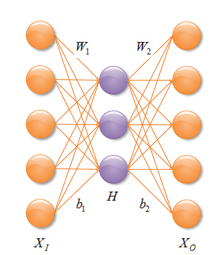
The structure of an autoencoder.
Figure 2 shows the structure of a SAE, in which the hidden layer output of the previous autoencoder is considered to be the input of the next autoencoder. Given input data, SAE can learn effectively representations from the original input and automatically filter unrelated features. Training SAE directly on the entire structure is very time-consuming and may cause the problem of gradient disappearance, especially in the case of large network depth. Layer-wise training has always been the core of deep neural network learning. For SAE, each autoencoder in SAE is first trained in a sequential and unsupervised manner through a back propagation algorithm. Since then, the updated parameters of SAE are shared. The SAE parameters can obtain local optimum values after layer-wise training. Moreover, SAE is not sensitive to the raw input features such that it does not require artificial feature extraction.
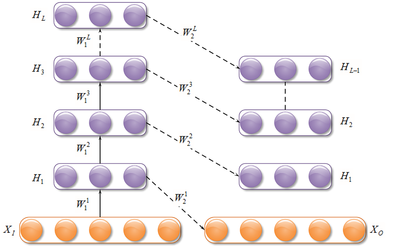
Stacked autoencoder structure.
Kernel ELM
ELM, proposed by Huang et al. (2006), is a SLFN. The ELM model has been widely used in many fields because of its high computational efficiency and generalization ability. The input weights and biases of the ELM model are randomly generated, and there is no need to adjust the hidden layer parameters. The output weights are obtained through a simple matrix computation, and this is why the ELM has high computing speed.
For N samples
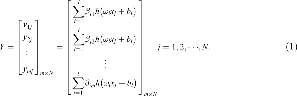
where

where H is the output matrix of the hidden layer. The only unknown parameter is the output weight

where

Then the output function of the ELM could be written as

This method overcomes some disadvantages of the typical gradient-based learning algorithms, such as overfitting, local minima, and long computation times. The topological structure of ELM is given in Figure 3.
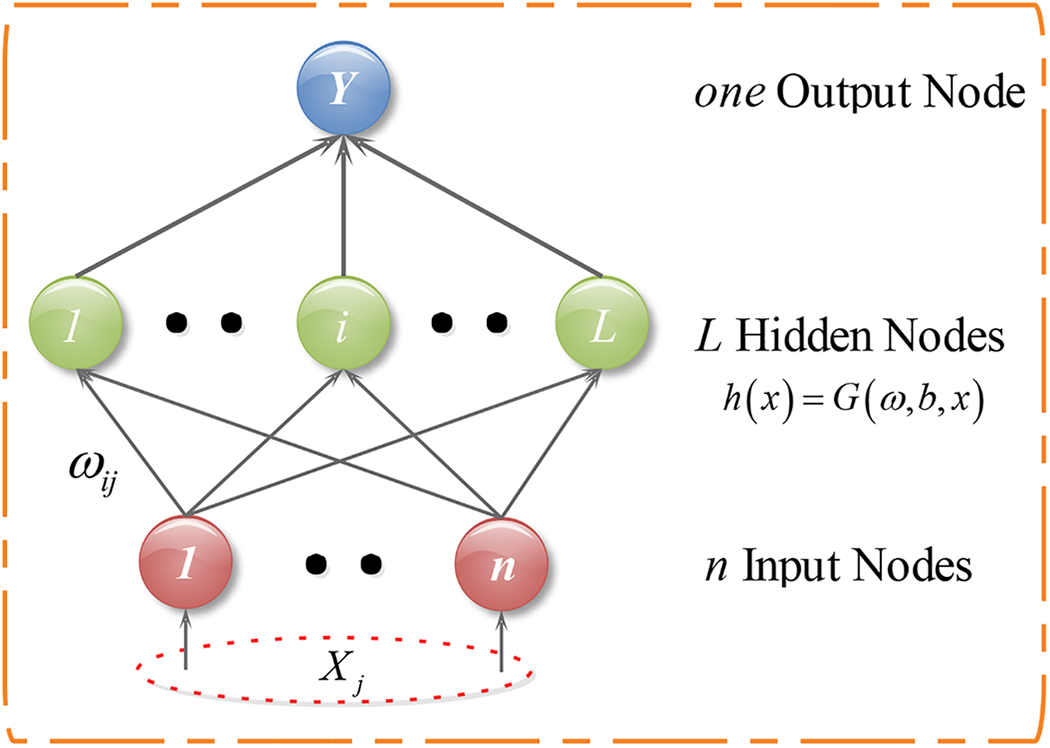
The topological structure of ELM. ELM: extreme learning machine.
Huang (2014) proposed a kernel-based ELM (KELM). According to Mercer condition, the activation function
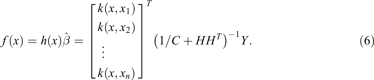
In the above formula, we do not need to know the feature mapping
SAKE flowchart. SAKE: stacked autoencoder with kernel-based extreme learning machine.
Bagging
Bagging (bootstrap aggregating) is originally developed by Breiman (1996) to improve the unstable process by generating new learning sets. The purpose of bagging is to reduce the variance of forecasting and thus lead to improved accuracy. Specifically, using the resampling method, bagging generates additional samples by extracting and replacing data from the original data to train the model. These additional samples are called resampling samples. We suppose that K samples are generated. For each resampling sample, the process described in the previous subsection for building the SAKE network is repeated and the forecasts will be generated in each iteration. Accordingly, we now have K sets of forecasts instead of one set of forecasts. To obtain the final forecast, we aggregate these K forecasts by taking the average or the median, and the forecast variance is lower than using only one original sample.
Bagging forecasting involves generating a great number of samples, called bootstrap samples. Let yt be the predictor vector at time t and
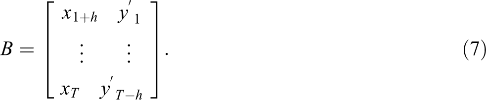
We generate a bootstrap sample k by giving a replacement from the matrix B blocks of m rows to capture the dependence in the error term. It can be expressed as follows:
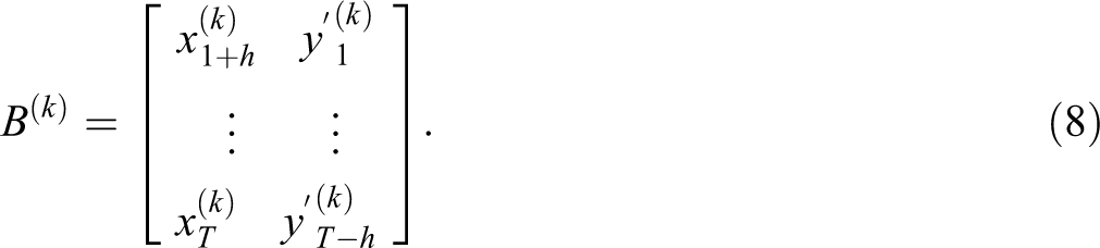
For each bootstrap sample, we perform model selection and estimate the model from matrix
For more details about bagging, please refer to Breiman (1996) and Athanasopoulos et al. (2017).
Multivariate forecasting
Multivariate forecasting, unlike univariate forecasting, takes the autoregressive effect of the target series and the impact of the exogenous variable into account. This can be denoted by

where
Ensemble deep learning approach
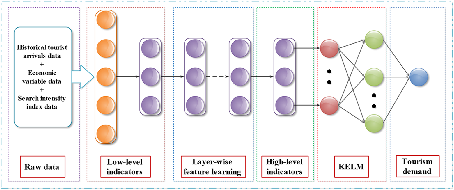
Figure 5 indicates the process of our proposed B-SAKE ensemble deep learning approach, which combines the advantages of bagging, SAE, and KELM. This approach is composed of the following five steps, which conforms to the general process of ensemble learning (Cao et al., 2020; Qiu et al., 2017; Zhao et al., 2017).
Step 1: Data preprocessing: transform and partition the original data into the in-sample data set (the training set) and the out-of-sample data set (the test set).
Step 2: Bootstrapping: generate K copies of the in-sample data sets by bagging approach.
Step 3: Model training: train K SAKE models with each copy of the in-sample data sets independently.
Step 4: Individual forecasting: generate K forecasts though using the K trained SAKE models.
Step 5: Aggregation: take the mean value of the K forecasts as the final forecasting results.
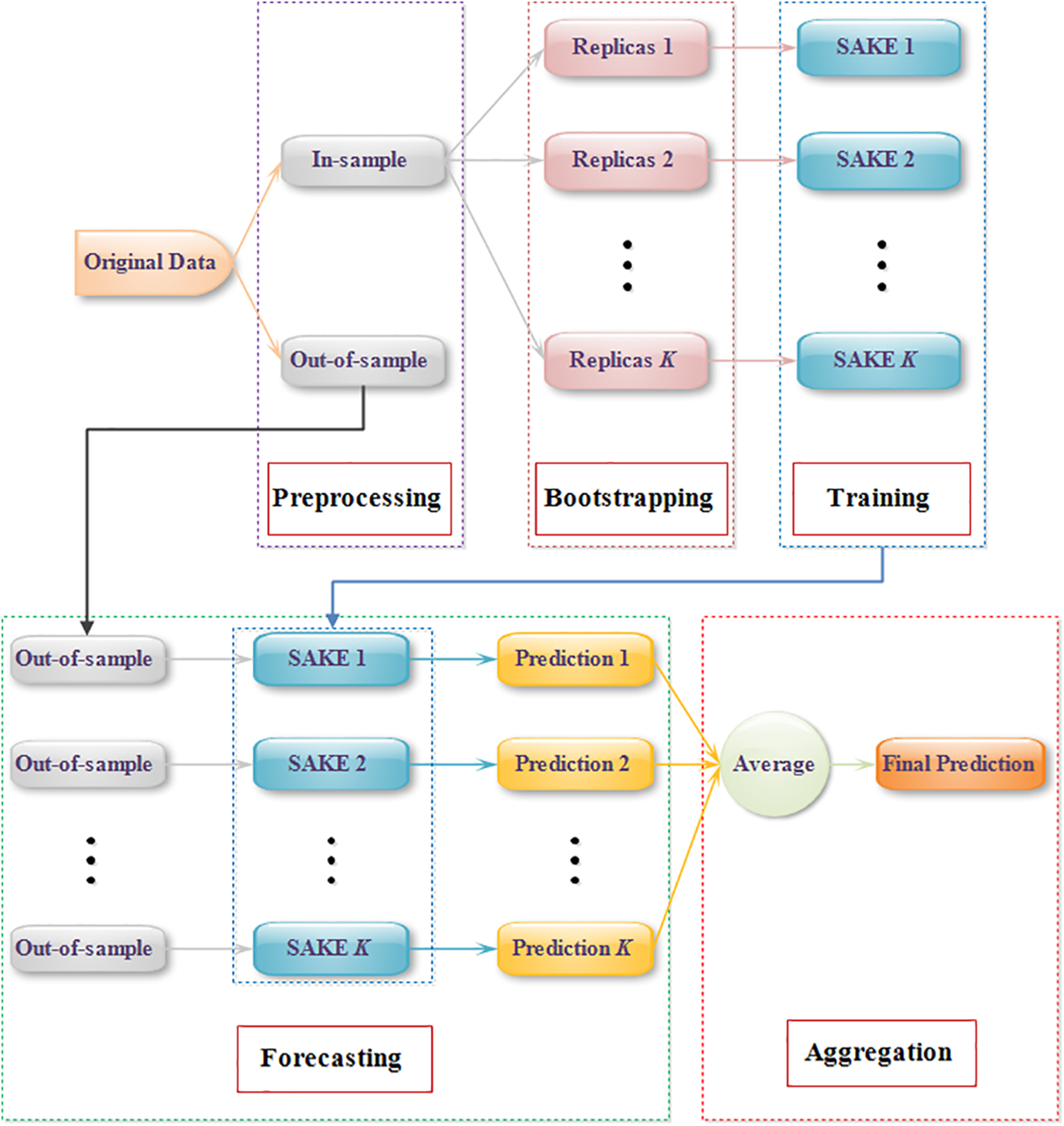
The process of B-SAKE ensemble deep learning approach. B-SAKE: bagging-based stacked autoencoder with kernel-based extreme learning machine.
Empirical study
This section provides a case study on Beijing tourist arrivals and compares the forecasting performance of our proposed B-SAKE with the benchmark models. “Data” section details the data sets involved in this study, including tourist arrival data, economic variables data, and SII data. “Performance evaluation criteria and statistic test” section describes the forecasting performance evaluation criteria and statistical tests. “Benchmarks and parameter settings” section introduces the benchmarks we choose and parameter settings. “Empirical results” and “Summary” sections give the forecasting results and reasonable interpretation.
Data
Tourist arrival data
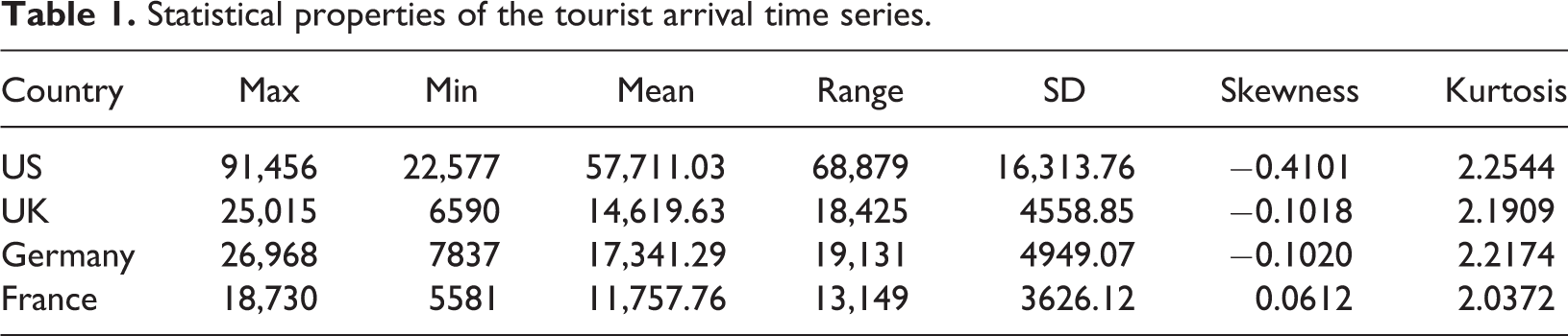
In this study, tourist demand (typically measured as tourist arrivals) is investigated for forecasting purposes. We select monthly inbound tourist arrivals in Beijing city over January 2008 to December 2018 from origin countries of the United States, the United Kingdom, Germany, and France, which is shown in Figure 6. It is observed that tourist arrivals show seasonality and volatility. The United States is the largest source of tourists for Beijing city within the four countries. Table 1 presents the statistical properties of the tourist arrival time series and indicates the difference in the statistical feature among the data sets. The tourist arrival data are obtained from the official website of the Beijing Municipal Bureau of Statistics (http://tjj.beijing.gov.cn/), which regularly publishes monthly tourist arrivals by nationality. The data sets are divided into the in-sample data set and the out-of-sample data set (see Figure 6). The in-sample data set serves as model training with data from 2008.1 to 2016.12, while the out-of-sample data set serves as model testing with data from 2017.1 to 2018.12. This division is consistent with the general laws of machine learning.
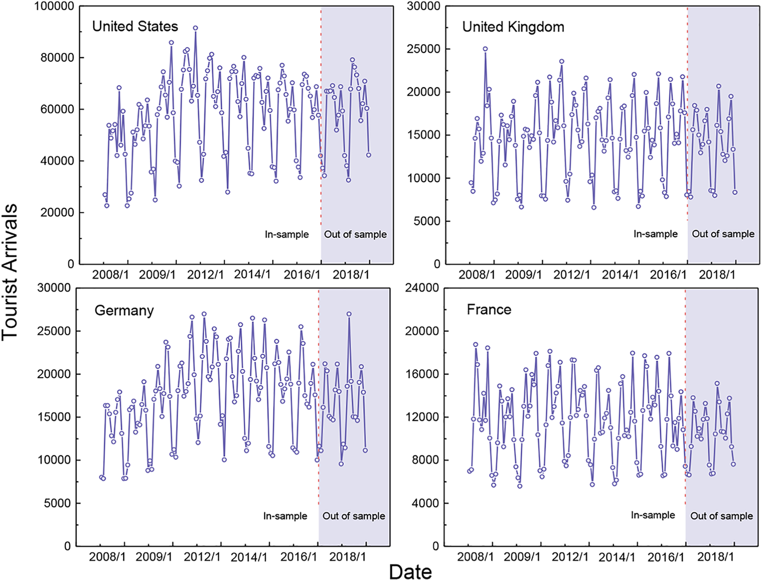
Tourist arrivals in Beijing city from four origin countries.
Statistical properties of the tourist arrival time series.
Economic variable data
Income and price are the basic variables of economic demand theory (Crouch, 1992). Income-like and price-like variables that have been extensively validated in the international tourism demand literature (Athanasopoulos et al., 2017; Li et al., 2005; Song and Li, 2008) include (1) income level of tourists, (2) future income expectations of tourists, (3) prices of the tourism products in the destination, and (4) prices of the tourism products in the substitute destinations. It is when income and price are considered at the same time that the tourists’ price perception of transnational tourism products could be accurately measured. Instead of constructing additional predictors, deep learning provides the possibility of end-to-end learning by directly utilizing typical income-like and price-like variables. This method not only greatly reduces the manual work but also avoids the loss of forecast accuracy. Considering the availability and reliability of data, we follow Athanasopoulos et al. (2017) and choose the following economic variables.
It is expected that tourists’ income level positively influences tourism demand. Tourist income level is usually measured in term of gross domestic product per capita

where
The interest rate spread reflects future economic activity and the business cycle (Anderson et al., 2007; Athanasopoulos et al., 2011; Athanasopoulos et al., 2017; Stock and Watson, 2012). Then future income expectations of tourists can be measured by the interest rate spread (IRS)

where
The demand of tourism product is inversely related to its price, which is indicated by the law of demand. The impact of exchange rates also needs to be considered for international tourism. We can use the price variable to measure this effect, which is defined as the ratio between the consumer price index (CPI) and standardized by the exchange rate
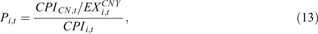
where
Furthermore, the demand of tourism product is also affected by the prices of other competing tourism products. International tourism demand literature indicates that similarities in climate, culture, and geography are indicative of substitute destinations (Kumar et al., 2020; Seetaram, 2012; Song et al., 2003). China, South Korea, and Japan are East Asian countries with similar climates, all influenced by Confucian culture, all have long histories and a large number of places of interest. Especially for European and American tourists, these three countries are typical destinations of Oriental culture tours (Noh and Vogt, 2013). Therefore, the substitute prices are defined as

where
The data of economic variables mentioned above are publicly accessible and can be downloaded via Wind (https://www.wind.com.cn).
SII data
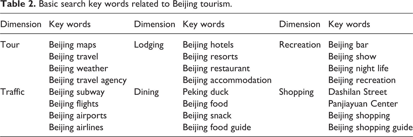
Following Yang et al. (2015) and Li et al. (2020), we choose 24 basic search key words in Google Trend based on the destination and various dimensions of tourism planning, including tour, lodging, recreation, traffic, dining, and shopping. The basic search key words related to Beijing tourism are listed in Table 2 with their corresponding dimensions. Then we search for the basic key words in a specific origin country and set iteratively recommended key words as the next time of search key words. We repeat this process until there are no new key words in the recommended list. Finally, we obtain 51, 45, 38, and 33 key words for the United States, the United Kingdom, Germany, and France, respectively.
Basic search key words related to Beijing tourism.
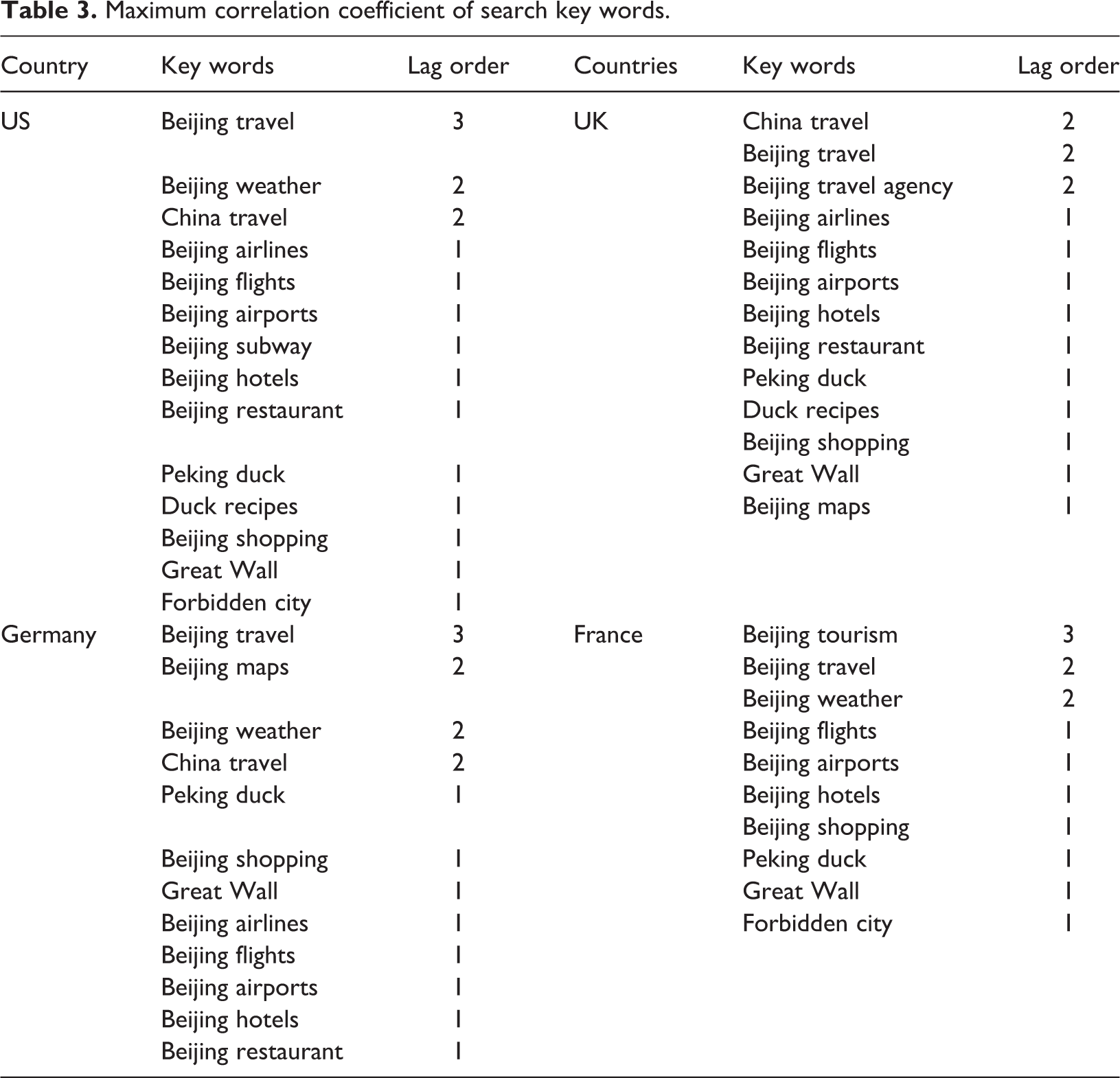
We calculate the Pearson correlation coefficient between tourist arrivals and key words with different lag periods. Four correlation coefficients are calculated for each of the key words, including the correlations between the visitor volumes in the current period and search query volumes from 1 to 3 months prior. We choose the key words with the highest correlation coefficient values, which are presented in Table 3. To obtain the appropriate key words, we use 0.7 as the threshold, in other words, we select the key words with a correlation coefficient value greater than 0.7. It can be observed that the optimal lag order of most key words is 1, indicating that tourists retrieve travel-related information one month in advance, which is consistent with our intuition.
Maximum correlation coefficient of search key words.
Performance evaluation criteria and statistic test
To evaluate and compare the forecasting performance of models, we adopt multiple error criteria commonly used in recent tourism demand forecasting literature (Law et al., 2019; Sun et al., 2019; Zhang, Li, et al., 2020, 2021), including MAPE, NRMSE, and DS. The specific formulas are written as follows:


where N is the number of observations in the data sets, xt and
To exclude the influence of the specific choice of data values in the sample, the Diebold-Mariano (DM) test and Pesaran-Timmermann (PT) test are employed to test the statistical significance of all models in the level forecasting and the directional forecasting, respectively. In the DM test, the MAPE is used as the loss function and thus the null hypothesis is that the MAPE of the test model is not less than that of benchmarks. The null hypothesis is rejected when DM statistics and the p value are less than the significance level. In the PT test, the null hypothesis assumes that the true and forecast values are independently distributed. Similarly, comparing PT statistics and the corresponding p value, the directional forecasting ability of different models can be evaluated from the statistical perspective. The process of the DM test and the PT test can be referred to Diebold and Mariano (1995) and Pesaran and Timmermann (1992).
Benchmarks and parameter settings
To evaluate the forecasting performance of the B-SAKE model in different forecasting schemes (one-step-ahead vs. multistep-ahead and in-sample vs. out-of-sample), we formulate 10 benchmark models, including univariate time series models, econometrics models, and AI models, of which the latter two are the multivariate models. Considering the seasonality and periodicity of tourism demand data, seasonal naive (SN), SARIMA, and seasonal exponential smoothing (SES) are chosen as univariate benchmarks. Due to the additional introduction of SII data and economic variable data, we also adopt a variant of SARIMA, namely SARIMAX (Tsui and Balli, 2015), which incorporates both seasonal influences and external variables. The autoregressive distributed lag (ARDL) model is also a common multivariate econometric model for tourism demand forecasting. The multilayer perceptron (MLP) and KELM models, as the most popular AI techniques, are widely used in the forecasting literature. We add SAE network for dimension reduction based on KELM to construct the SAKE model. In addition, we consider bagging-based (B-based) AI models including B-MLP, B-KELM, and B-SAKE.
The parameter specification is crucial for model performance. We adjust the parameters through minimizing in-sample forecasting errors. The appropriate parameters of SES, SARIMA, SARIMAX, and ARDL model are estimated according to Akaike’s information criterion. The numbers of hidden neurons of MLP and KELM are determined by the trial-and-error approach. The Gaussian kernel function is adopted in the KELM model. And the bootstrap samples of Bagging are set as 100 based on Inoue and Kilian (2008).
Empirical results
Forecast evaluations
We adopt the dynamic forecasting with rolling windows. For in-sample data and out-of-sample data, the first 12 observations are used to fit and forecast the next value, respectively. In the one-step-ahead forecasting, the window rolls forward one step each time, while in the multistep-ahead forecasting, the corresponding number of steps is rolled forward each time. After obtaining the results of the dynamic forecasting, we use the predicted and actual tourism arrivals for each origin country to calculate the average error rate for each evaluation criteria (MAPE, NRMSE, and DS). The multistep-ahead forecasting in this study includes 3-month-ahead forecasting and 6-month-ahead forecasting. To verify the effectiveness of bagging and SAE in dealing with overfitting and improving forecasting performance, we also design a comparison between in-sample forecasting and out-of-sample forecasting.
We evaluate the forecasting performance of our proposed B-SAKE model and the above 10 benchmark models in the above forecasting schemes using the MAPE, NRMSE, and DS evaluation criteria. The results are presented in Tables 4–6 and it can be summarized that (1) B-SAKE is the most accurate approach compared with the benchmark models in terms of the MAPE, NRMSE, and DS criteria. (2) The B-based models generally outperform the original models in forecast accuracy, which verifies bagging’s superiority in tourism demand forecasting. (3) As we expected, SAKE, combining SAE and KELM, has better forecasting performance than KELM. SAE automatically and effectively identifies data characteristics through dimensionality reduction. (4) The univariate models (i.e. SN, SARIMA, and SES) are the worst benchmark models, followed by the econometric models (i.e. ARDL and SARIMAX). This may be because these models cannot effectively capture the nonlinear patterns of tourism data compared with the AI models. In addition, the univariate models fail to take advantage of the effective information of tourism big data. (5) Although almost all model performance degrades from in-sample forecasting to out-of-sample forecasting, bagging and SAE significantly mitigate this problem, especially in one-step-ahead forecasting.
Forecasting performance of different models: 1-month-ahead forecasting.
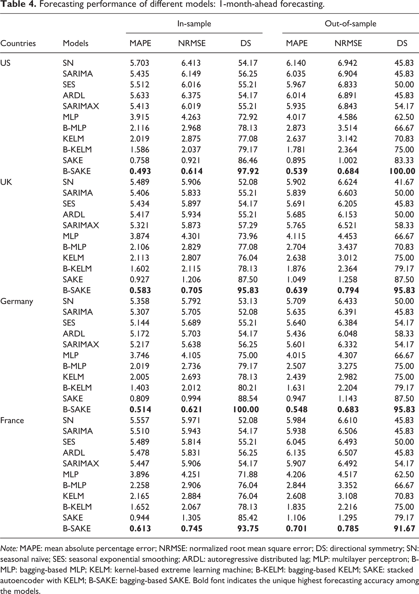
Note: MAPE: mean absolute percentage error; NRMSE: normalized root mean square error; DS: directional symmetry; SN: seasonal naïve; SES: seasonal exponential smoothing; ARDL: autoregressive distributed lag; MLP: multilayer perceptron; B-MLP: bagging-based MLP; KELM: kernel-based extreme learning machine; B-KELM: bagging-based KELM; SAKE: stacked autoencoder with KELM; B-SAKE: bagging-based SAKE. Bold font indicates the unique highest forecasting accuracy among the models.
Forecasting performance of different models: 3-month-ahead forecasting.
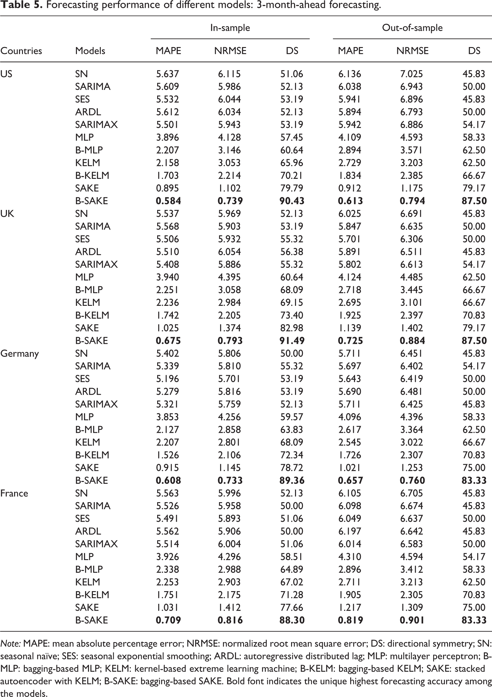
Note: MAPE: mean absolute percentage error; NRMSE: normalized root mean square error; DS: directional symmetry; SN: seasonal naïve; SES: seasonal exponential smoothing; ARDL: autoregressive distributed lag; MLP: multilayer perceptron; B-MLP: bagging-based MLP; KELM: kernel-based extreme learning machine; B-KELM: bagging-based KELM; SAKE: stacked autoencoder with KELM; B-SAKE: bagging-based SAKE. Bold font indicates the unique highest forecasting accuracy among the models.
Forecasting performance of different models: 6-month-ahead forecasting.
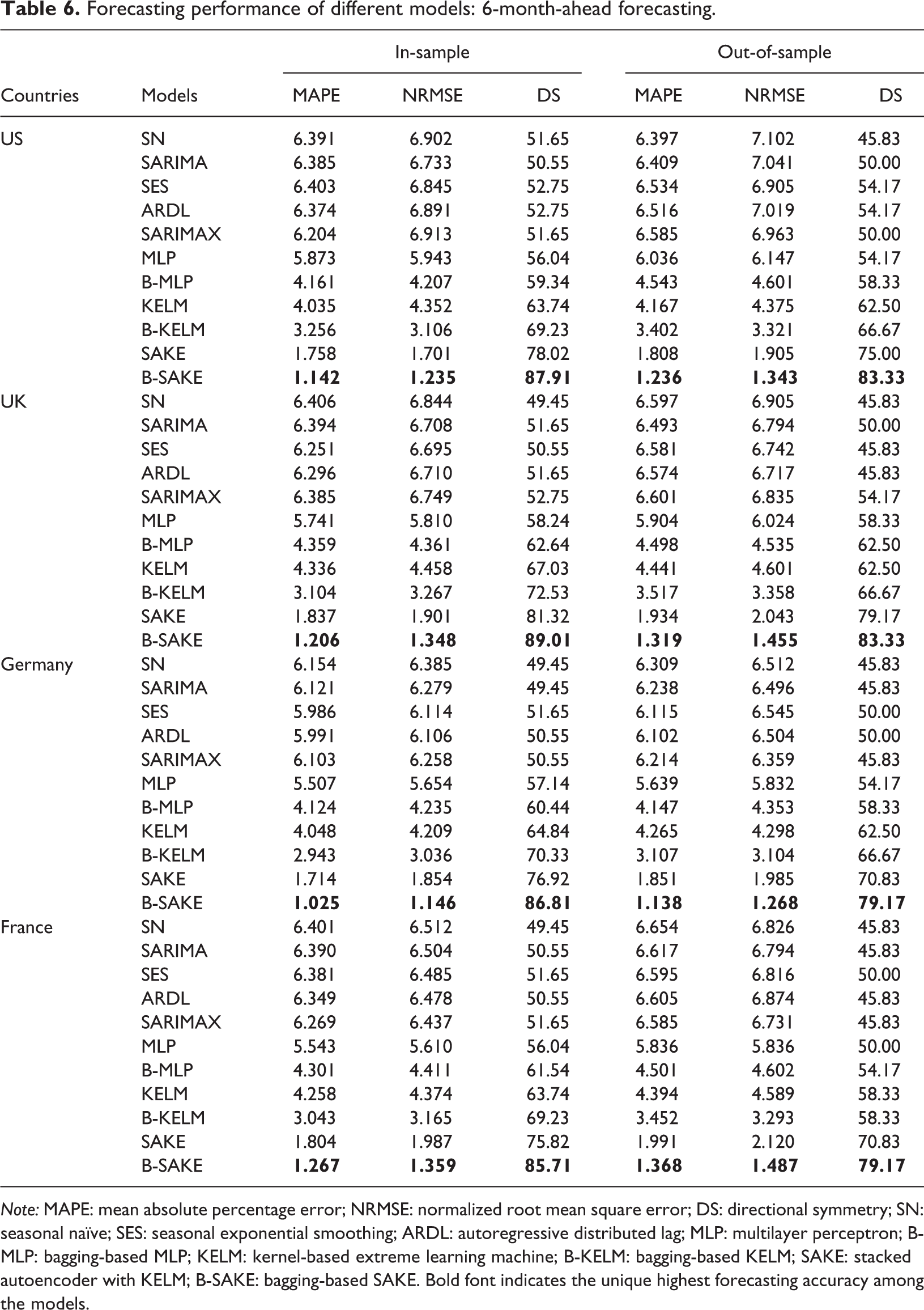
Note: MAPE: mean absolute percentage error; NRMSE: normalized root mean square error; DS: directional symmetry; SN: seasonal naïve; SES: seasonal exponential smoothing; ARDL: autoregressive distributed lag; MLP: multilayer perceptron; B-MLP: bagging-based MLP; KELM: kernel-based extreme learning machine; B-KELM: bagging-based KELM; SAKE: stacked autoencoder with KELM; B-SAKE: bagging-based SAKE. Bold font indicates the unique highest forecasting accuracy among the models.
In particular, our proposed B-SAKE model achieves the best forecast accuracy in all four origin countries, which is shown in bold in the tables. Taking the example of the case of 1-month-ahead forecasting in the United States, the reductions in MAPE are 91.22%, 91.07%, 90.97%, 91.04%, 90.92%, 86.58%, 81.24%, 79.56%, 69.74%, and 39.78% in comparison with those of SN, SARIMA, SES, ARDL, SARIMAX, MLP, B-MLP, KELM, B-KELM, and SAKE, respectively. For NRMSE, the reductions are 90.15%, 90.09%, 89.99%, 90.07%, 90.00%, 85.09%, 80.54%, 78.23%, 71.07%, and 31.74%, respectively. B-SAKE achieves 84–118% better directional forecasts than the univariate models or econometric models and 20–60% better directional forecasts than the AI models. From in-sample forecasting to out-of-sample forecasting, the accuracy loss of MAPE after applying bagging on the SAKE decreases from 18.07% to 9.33%, compared with that of the SAKE without bagging. Analogously, SAE helps KELM reduce the accuracy loss of MAPE from 30.61% to 18.07%. It is clearly illustrated that the B-SAKE model is a highly promising forecasting approach.
Statistic tests
To further verify the level and directional forecasting performance of the B-SAKE model from the statistical perspective, the DM test and the PT test are also employed to test the statistical significance of all the models within the out-of-sample data. Tables 7–12 report the results of the DM test and the PT test with respect to different forecasting horizons. The numbers outside the brackets in the tables are the DM statistics or PT statistics while the numbers inside the brackets are the corresponding p values.
The DM test results for B-SAKE versus univariate forecasting models.
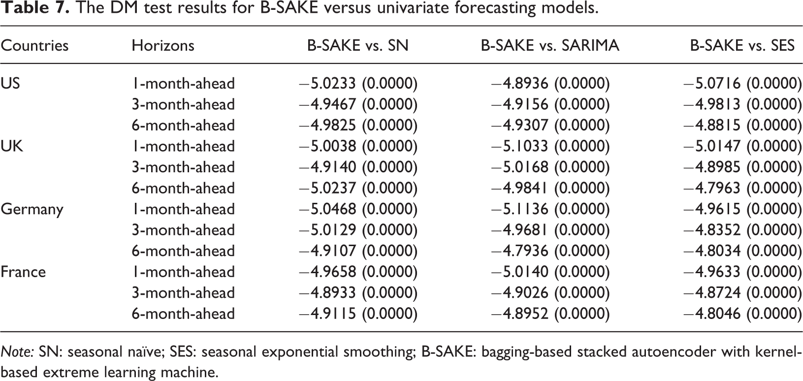
Note: SN: seasonal naïve; SES: seasonal exponential smoothing; B-SAKE: bagging-based stacked autoencoder with kernel-based extreme learning machine.
The DM test results for multivariate forecasting models in 1-month-ahead forecasting.
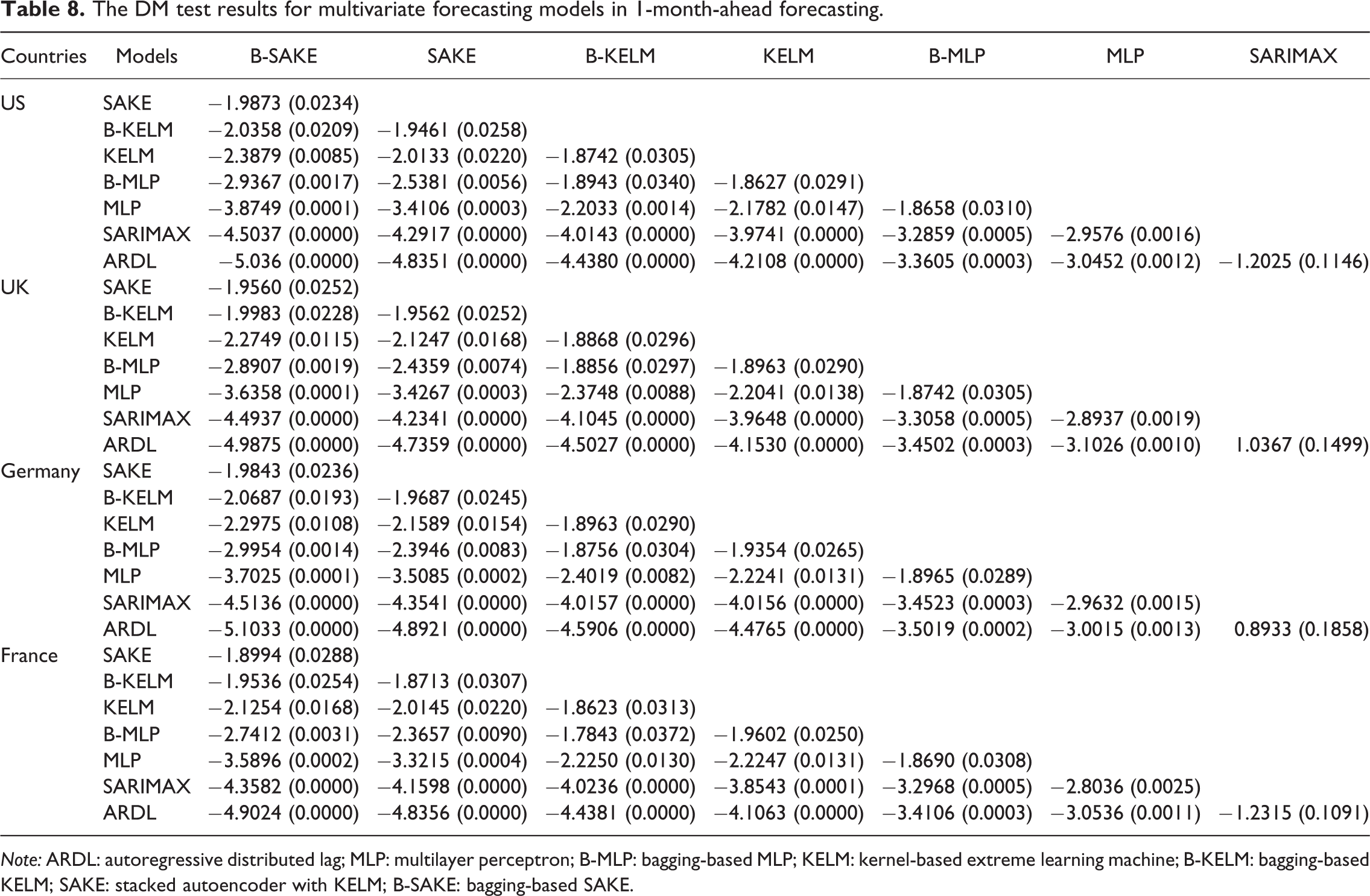
Note: ARDL: autoregressive distributed lag; MLP: multilayer perceptron; B-MLP: bagging-based MLP; KELM: kernel-based extreme learning machine; B-KELM: bagging-based KELM; SAKE: stacked autoencoder with KELM; B-SAKE: bagging-based SAKE.
The DM test results for multivariate forecasting models in 3-month-ahead forecasting.
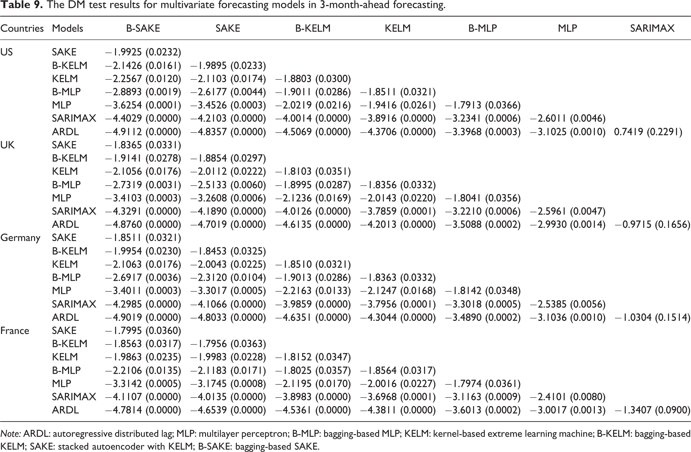
Note: ARDL: autoregressive distributed lag; MLP: multilayer perceptron; B-MLP: bagging-based MLP; KELM: kernel-based extreme learning machine; B-KELM: bagging-based KELM; SAKE: stacked autoencoder with KELM; B-SAKE: bagging-based SAKE.
The DM test results for multivariate forecasting models in 6-month-ahead forecasting.
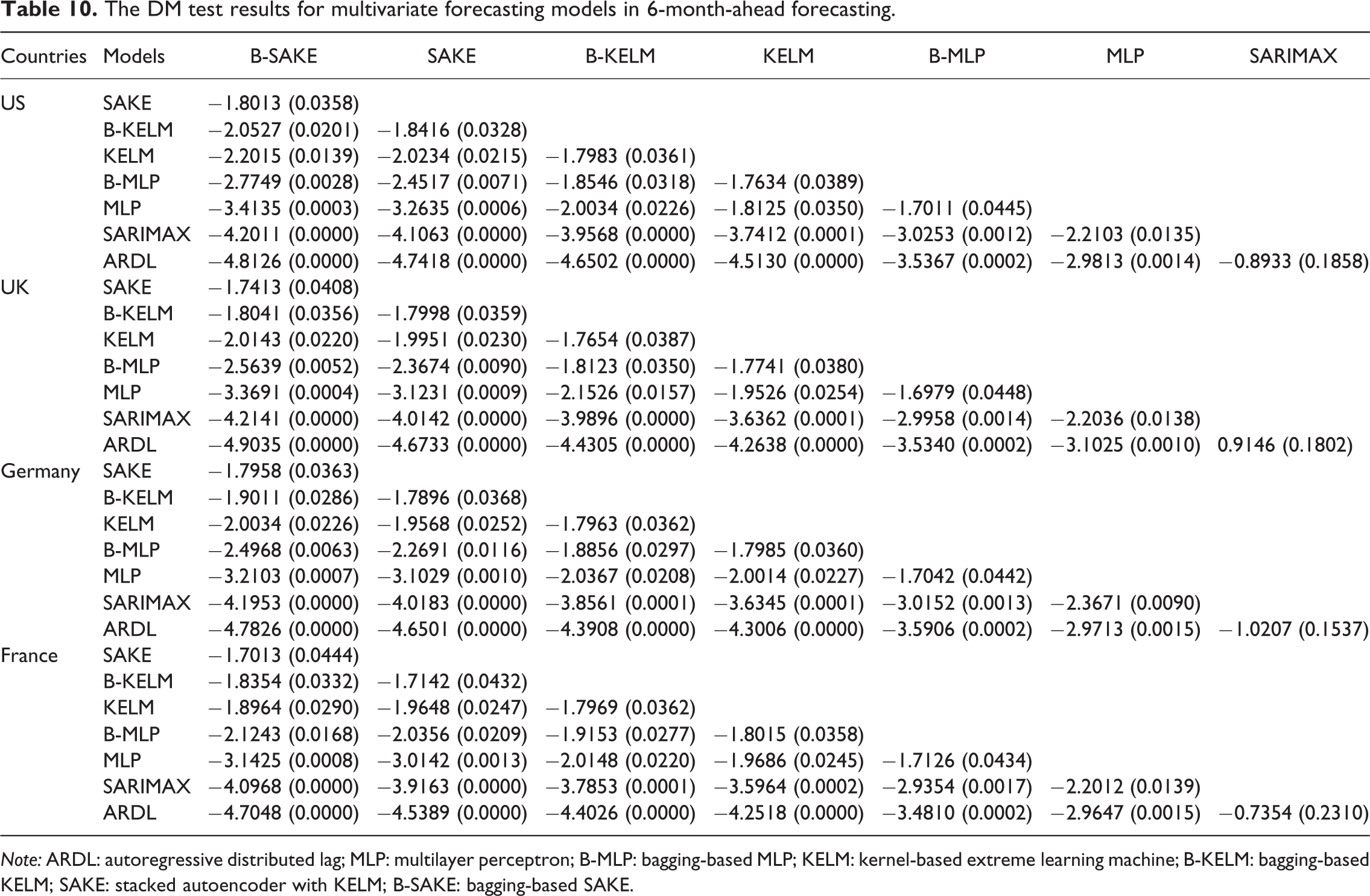
Note: ARDL: autoregressive distributed lag; MLP: multilayer perceptron; B-MLP: bagging-based MLP; KELM: kernel-based extreme learning machine; B-KELM: bagging-based KELM; SAKE: stacked autoencoder with KELM; B-SAKE: bagging-based SAKE.
The PT test results for univariate forecasting models.
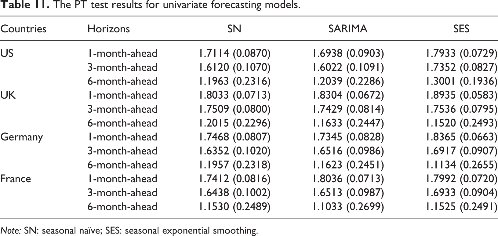
Note: SN: seasonal naïve; SES: seasonal exponential smoothing.
The PT test results for different models.
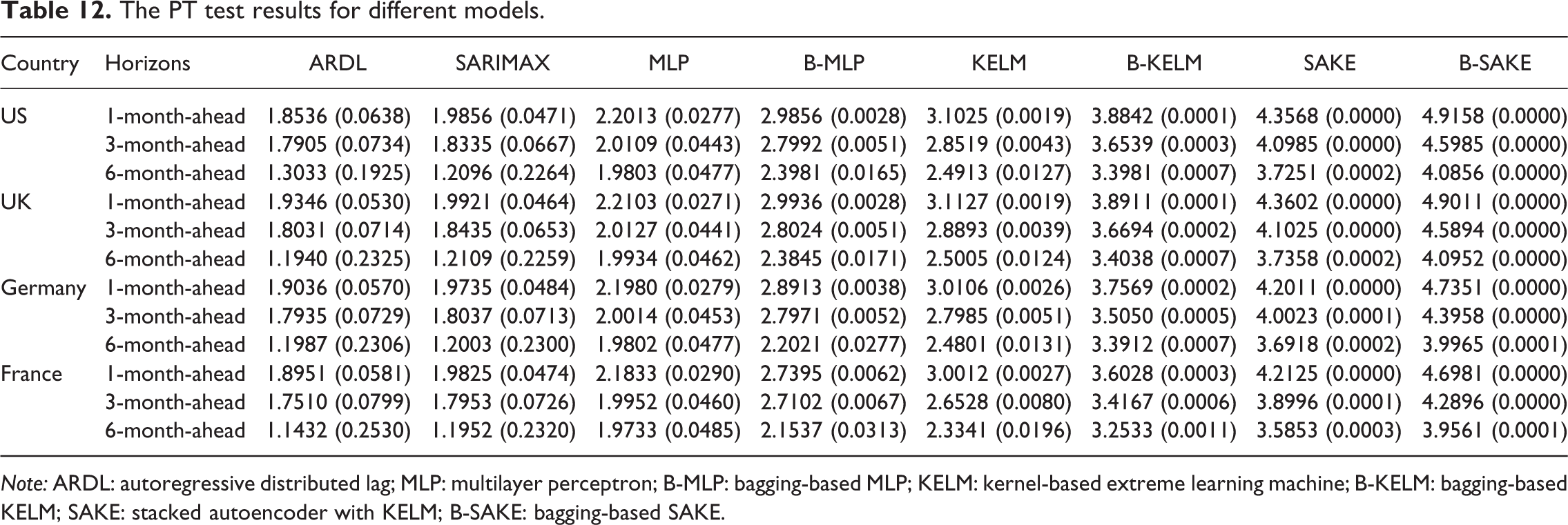
Note: ARDL: autoregressive distributed lag; MLP: multilayer perceptron; B-MLP: bagging-based MLP; KELM: kernel-based extreme learning machine; B-KELM: bagging-based KELM; SAKE: stacked autoencoder with KELM; B-SAKE: bagging-based SAKE.
According to the DM test results (Table 7–10), when testing the B-SAKE model, all the DM tests are less than −1.7013 corresponding to p values less than 0.0444, which means that the B-SAKE model outperforms the benchmark models under the 95% confidence level. This indicates the superiority of the B-SAKE model. Specifically, we note that when the B-SAKE is tested against the univariate models and econometrics models, the B-SAKE model statistically confirms its superiority under the 100% confidence level. Furthermore, Tables 8–10 present that the level forecasting performance of the models increases successively for MLP, B-MLP, KELM, B-KELM, SAKE, and B-SAKE in multistep-ahead forecasting scheme. B-based models and SAE-based models outperform the original models under the 95% confidence level, which demonstrates the effectiveness of bagging and SAE.
The results of the PT test are displayed in Tables 11 and 12. The forecasting results of the B-KELM, SAKE, and B-SAKE models reject the null hypothesis in both one-step-ahead forecasting and multistep-ahead forecasting under near the 100% confidence level, which indicate the powerful performance of these three models in the directional forecasting. The B-SAKE performs the best in all forecasting schemes, followed by the SAKE, B-KELM, KELM, B-MLP, and MLP. The univariate models and econometrics models are almost ineffective in multistep-ahead forecasting where their p values are greater than 0.1. Bagging and SAE can significantly improve performance in the directional forecasting.
Summary
In this section, we train the models and conduct numerical experiments employing the multidimensional data related to tourism demand, including historical data on tourist arrivals in Beijing from four countries, economic variable data, and SII data. The forecasting results of our proposed B-SAKE model and benchmark models are compared through different forecasting schemes. In summary, some interesting implications are obtained as follows. The proposed B-SAKE model achieves the highest forecast accuracy via MAPE, NRMSE, and DS and outperforms the benchmark models in the DM test and the PT test, followed by other AI models, whereas the univariate models and econometrics models rank the last. The univariate models and econometrics models are not applicable to forecasting nonlinear, uncertain, and irregular tourism data, while nonlinear AI models have significant advantages. As an ensemble approach, bagging can effectively mitigate overfitting and improve the forecast accuracy through the idea of the model average. The SAE is utilized to construct the deep learning network realizing feature recognition effectively. This study analyzes the forecasting performance of the models based on tourist arrival data in Beijing from four countries and comes to almost consistent conclusions, which illustrates the effectiveness and robustness of this model framework.
Discussion
Considering the tourism big data, a bagging-based multivariate ensemble deep learning model, integrating SAE and KELM, is proposed for tourism demand forecasting. The data applied in this article include historical data on tourist arrivals in Beijing, economic variable data, and SII data. The empirical study results indicate that our proposed B-SAKE model substantially outperforms the benchmark models in different forecasting schemes (one-step-ahead vs. multistep-ahead and in-sample vs. out-of-sample). In particular, we analyze the cases of forecasting tourist arrivals from four countries and reach consistent conclusions. Moreover, bagging and SAE in the ensemble deep learning model framework designed by us effectively solve the overfitting problem and improve the forecasting accuracy by increasing the data volume and improving the feature extraction efficiency, respectively.
The ensemble deep learning model we propose has significant implications for relevant government officials and tourism practitioners. This accurate and reliable forecasting model assists these stakeholders to design and implement effective policies and strategies to meet the potential needs of tourists, thus improving the quality of tourism services and the competitiveness of destinations. In addition, this ensemble deep learning model framework can be performed to forecast other complex problems, for instance, passenger flow forecasting, electric load forecasting, and financial market forecasting.
The limitation of this study is that other newly developed deep learning models in the tourism forecasting literature don’t serve as benchmark models. This is because the details of model construction have not been clearly stated in previous literature, and few shared data sets contributing to comparability. Fortunately, Zhang, Li, et al. (2021) have noticed this issue and release their data set on GitHub. Additionally, it is worth noting that weather, safety factors, and online comment data have been taken into consideration in the tourism demand literature (Chen et al., 2015; Ghaderi et al., 2017; Sohrabi et al., 2020). These data can theoretically be incorporated into our proposed B-SAKE model to further improve the forecast accuracy. It is also meaningful to explore the preprocessing of these types of data and the construction of indicators related to tourism demand.
Footnotes
Declaration of conflicting interests
The author(s) declared no potential conflicts of interest with respect to the research, authorship, and/or publication of this article.
Funding
The author(s) disclosed receipt of the following financial support for the research, authorship, and/or publication of this article: This research work was partly supported by the National Natural Science Foundation of China under Grants No. 71988101 and No. 71642006, the Fundamental Research Funds for the Central Universities under Grant No. SK2021007.