
Abstract
This research investigates the optimum spatial scale of regional tourism cooperation based on the tourism flows spillover in Mainland China. Using panel data from 341 prefecture-level cities in Mainland China, spatial econometric modeling is employed to estimate the spillover effects to determine the optimum spatial scale of regional tourism cooperation. The findings reveal that there are spatial correlations of tourism flow. In addition, tourism economic fundamental factor, surrounding market factor, tourism transportation facility factor, and tourist attraction factors have a positive and significant impact not only on local tourism flows but also on the surrounding areas. Finally, it is found that the optimum spatial scale of the regional tourism cooperation in Mainland China is [5, 15] cities, whereas for the eastern, western, southern, and northern regions, the optimum scale of the regional tourism cooperation is [5, 21], [5, 26], [5, 26], and [5, 11] cities, respectively.
Keywords
Introduction
Considering the development of economic globalization and regional integration, regional cooperation has become an inevitable trend and remains in process (Fritsch and Franke, 2004; Kohsaka, 2004; Sato, 1995; Uddin and Taplin, 2015). The tourism economy is an important part of economic development and regional tourism cooperation is an unsurprising avenue for tourism development (Fagence, 1996). Under such a background, seeking regional cooperation to achieve resource integration, market sharing, and information exchange to form a regional amplification effect has become a new development trend of the global tourism economy (Lin et al., 2020). Since its reform and opening-up, the Chinese tourism industry has rapidly developed, the scale of which has continued to expand, and the industrial system has become increasingly complete. In 2019, the number of individual Chinese tourists in China was 6.006 billion, the number of outbound tourists was 155 million, and the number of inbound tourists was 145 million. The total annual tourism revenue was 6.63 trillion yuan, which indicates an annual increase of 11%.
Meanwhile, the disorderly competition in the tourism market has also induced regional tourism cooperation (Dong et al., 2012; Li et al., 2020; Lin et al., 2020; Theocharous et al., 2020). Regarding tourist destinations, with the development of the tourism economy, competition among destinations has become increasingly fierce. Tourism activities are indeed regional, and the intense rivalry among the subjects of regional tourism has led to the repeated construction of tourism resources and similar products (Li et al., 2020), thus deepening the competition. If these circumstances continue, the tourism industry will eventually enter a vicious circle. From the perspective of tourists, with the improvement of material and spiritual living standards, people’s requirements for tourist activities have also demonstrated diversified and complicated characteristics. Tourists hope to obtain more and richer experiences in each journey (Fagence, 1996). Moreover, tourists pay more attention to the quality of tourism, and tourists’ consumption tends to be more rational. To alleviate this disorderly competition and effectively satisfy the diverse needs of tourists, various regional tourism cooperation organizations of different levels and scales are constantly appearing at home and abroad. The most successful international case is the integration of tourism in the European Union. In China, there is mature regional tourism cooperation, such as the Yangtze River Delta, the Pearl River Delta, and Huang-Huai-Hai (Duan et al., 2020). After experiencing the three stages of scenic spot competition, route competition, and city competition, the regional competition of Chinese tourism has entered a new era of inter-regional coordination and cross-regional competition (Li et al., 2020). Regional integration has become the basic unit of tourism competition. To maximize their interests in a fiercely competitive environment, tourist destinations must enhance their competitiveness through alliances, expansion, resource integration, and brand innovation, as well as attract tourists from inside and outside the region.
Regional tourism cooperation can achieve effective resource-sharing, market expansion, cost reductions, scaling of economies, and effects that the overall is greater than the sum of the parts (Arroll, 1993; Guoand He, 2012). This cooperation is an inevitable choice for regional economic development and is a significant way to improve tourism competitiveness and build tourism destination brands. However, as a spatial organization with a certain geographic scope, the optimum scope (or scale) of regional tourism cooperation is important. If the scale is too large, the tourism resources within the cooperation scope will not be fully utilized, which will result in a waste of resources. Contrarily, if the scale is too small, it will not be able to satisfy the needs of tourists, which is also not conducive to the healthy development of regional tourism cooperation (Costa and Lima, 2018; Fagence, 1996).
Considering the existing research on regional tourism cooperation at home and abroad, most scholars only stop at the construction and spatial structure of regional tourism cooperation, although some have realized the importance of the spatial scale (Hascoët, 2019; Li et al., 2020; Wang, 2009), and use various qualitative or quantitative methods to explore. However, some deficiencies remain: (1) in the qualitative research, only the approximate scale of the regional tourism cooperation is provided, and no explanation is given as to whether the scale of the regional tourism cooperation is appropriate; (2) in the quantitative research, either the spillover effect between regions is not considered or the spillover effect between multiple destinations could not be described simultaneously; and (3) previous methods do not consider the relevance of the geographic space. According to the first law of geography, a correlation lies between everything. The closer the distance between two things, the greater their correlation. Contrarily, the farther the distance between two things, the weaker their correlation. Therefore, the spatial correlation of geographic location plays a significant role in the construction of regional tourism cooperation. Based on this, we introduce the spatial econometric model, which assigns a spatial weights matrix to the tourism flows of neighboring cities/regions as a spatially lagging dependent variable and introduces it into the traditional econometric model. The regression coefficient (i.e., spillover coefficient) is used to measure the spillover effect of tourism flows (Yang and Wong, 2012). Among them, the definition of “neighbors” by the spatial weights matrix provides an effective way to measure the optimum scale of regional tourism cooperation. Specifically, this means setting different numbers of neighbors to perform scenario simulations to calculate the spillover effect under the corresponding scenarios. This is done to analyze the “optimum scale” of the regional tourism cooperation by establishing a quantitative relationship between the “number of neighbors” and the “spillover effect.”
So, we choose China as our context. As a pillar industry of the national economy and modern service industry in China, the tourism industry has witnessed rapid growth in recent years. Specifically, the total revenue from the tourism industry reached 6.0 trillion Yuan, which accounted for about 11.0% of China’s GDP in 2018. More importantly, these numbers are on the rise. In this context, for the relevant stakeholders, to further accelerate the high-quality development of the tourism industry in all regions of China, the regional tourism cooperation launched by local governments is playing an irreplaceable role in promoting the development of the regional tourism industry. For instance, as one of the most economically developed regions in China, the Yangtze River Delta has become a typical demonstration area for regional tourism cooperation. However, the scale of its cooperation expanded was continuously from the initial 16 cities in 2003 to 20 cities in 2004, 24 cities in 2005, and 25 cities in 2006. In other words, the scale of the cooperation is mainly determined by the subjective will of local governments, and whether the scale is optimal remains to be discussed. Similar issues could be found elsewhere in China. Therefore, for the relevant stakeholders, how to determine their optimum scale is of great significance for promoting the sustainable development of China’s tourism industry. This is also the main reason why this paper takes China as our research object. Moreover, for the relevant policy makers in other market economies such as India and Brazil, it might also provide an important reference to formulate more targeted measures for improving the development of the regional tourism industry.
The article is organized as follows: after the introduction, relevant literature is reviewed, including that which focuses on tourism spillover effects and the methods examining tourism flows spatial spillover. Based on past research, the stepwise regression and spatial econometric method are then detailed, with a description of the study’s research region and corresponding empirical data. Subsequently, the optimum scales of regional tourism cooperation in Mainland China and the different regions are presented and discussed. Finally, conclusions are provided.
Literature review
The spillover effect of tourism flows
The spillover effect represents a concept of externality. When an individual or organization takes a certain behavior, it affects not only itself but also the others, which means that this activity will produce an effect that the activity subject cannot enjoy (Sun and Wang, 2014; Zhang et al., 2020). As two basic types of spillover effects, knowledge spillover and technology spillover represent the internal mechanism of the effect. Knowledge spillover is proposed by Romer, who believes that the difference between knowledge and general commodities is that knowledge has a spillover effect and is beneficial to learning and communication between people. Moreover, it is transmitted invisibly (Hollanders and Weel, 2002). Kokko (1992) believes that demonstration and competition are the sources of technology spillover effect. Whether it is knowledge spillover or technology spillover, both will have a diffusion effect on economic activities and form an inter-regional linkage development. The tourism spillover effect is a concept of externality. It represents the positive or negative effect of a certain city/region on others in the tourism economic development (Yang et al., 2017; Yang and Fik, 2014; Yang and Wong, 2012; Zhou et al., 2017). The construction of regional tourism cooperation is an attempt to use tourism spillover effects to internalize it, thereby enhancing the overall development level of regional tourism. Accordingly, the size of the tourism spillover effects can become a certain “scale” for judging the effect of regional tourism cooperation. If the “internalization” of the tourism spillover effects under a certain tourism cooperation scale is the most significant and effective, the cooperation scale is theoretically the “optimum scale” of the regional tourism cooperation.
In fact, the tourism spillover effects, as the core internal force affecting the tourism cooperation of the regions and cities (Gooroochurn and Hanley, 2005), have received increasing attention from scholars (Lazzeretti and Capone, 2009; Li et al., 2020), such as the spillover effects of tourism and tourism employment (Capone and Boix, 2008) as well as the spillover effects of economic growth of tourism (Tian et al., 2021; Yang and Fik, 2014). However, studies on the optimum scale of regional tourism cooperation are scarce. The traditional method of exploring the spatial scale of this collaboration is mainly based on the “core–periphery” theory to qualitatively describe the “boundary” of the tourism destination (Li et al., 2020). However, among the two basic types of the spatial structure of regional tourism cooperation, emphasis should not only be placed on the role of the center-hinterland structure of “spatial dependence” but also on the importance of the hub-network structure of “functional connections” between nodes. In reality, this is manifested as a composite of these two structures. The attempt to define the spatial scale of the regional tourism cooperation based solely on the “core–periphery” theory would be theoretically incomplete. Meanwhile, the “degree of optimum” of the spatial scale requires both a qualitative interpretation and a quantitative measurement of this “degree” technically, so as to provide practical guidance to the construction and practice of the regional tourism cooperation (Kibicho, 2009). The related research on tourism spillover effects provides an effective way to perform this quantitative measurement.
Methods examining tourism flows spatial spillover
Simultaneous equation method
The simultaneous equation method calculates other unknown variables in the system by simultaneously solving all the equations of a steady-state process system (Kai, 1998). This method takes solving equations as the main idea and uses the least-squares method as the estimation method; it is widely used in the research of economic problems, and some scholars later introduced it into the tourism field. Tse (1999) observed a close link between the number of tourists, tourism receipts, and spending, as well as subsequent private domestic consumption. Zamparini et al. (2017) analyzed the impact of economic variables and noneconomic factors on tourism demand in 99 Italian regions from 1998 to 2003. The analysis reveals that the considered variables have significant effects on the evolution of tourism demand, with climate, tourism supply, and entrepreneurial capacity having the greatest impact. The model related to the simultaneous equation model is the Mundell–Fleming model (MF). Mundell and Fleming established the MF model in the 1960s to study financial and monetary issues under the market economy (Fleming, 1962; Mundell, 1962). Since their endeavors, the model has been continuously revised and applied to GDP research. In 2008, Li and Huang (2008) introduced the MF model to the spillover effect of regional tourism economy using tourism income in different regions as a variable to discuss the regression coefficient in the model. Moreover, this coefficient was used as an indicator to measure the inter-regional tourism spillover. Accordingly, the MF model has been applied to the field of tourism development.
Seemingly unrelated regression estimation
The seemingly unrelated regression estimation is similar to the equation-oriented method. An inherent correlation does not exist among the variables of the model; rather, it lies in the disturbance terms of the equations. This model was first processed in the analysis of a company’s annual investment problems (Zellner, 1962). Subsequently, it has been revised and optimized to solve complex economic problems across myriad fields. In the analysis of tourism-related research topics, Crouch employed this idea in 1994 to study tourism demand (Crouch, 1994). Meanwhile, Tihomir asserted that the seemingly uncorrelated regression estimates are more accurate in inferring and forecasting tourism demand. In addition, Gooroochurn and Hanley measured tourism spillovers in Northern Ireland and the Republic of Ireland, validated the existence of inter-regional tourism spillover effects, and measured the strength of this effect using a quantitative approach. However, they pointed out that the applicability of this method was not high for the study of tourism spillovers among multiple regions (Gooroochurn and Hanley, 2005).
Gap model
Based on the new growth theory and technology gap theory, Caniëls and Verspagen (2003) emphasized the importance of spatial proximity to the spread of knowledge and technology. Moreover, they defined and modeled it. Drawing on this model, based on the similarities among knowledge, technology, and tourism products, Deng et al. (2003) proposed a conceptual model of regional tourism spillover. Accounting for the differences of tourism products, the spatial distance is regarded as the distance gap and the grade and type difference of tourism products as the grade gap and type gap, respectively, to construct the model, which is the gap model. More recently, Shen (2020) verified the overflowing measure of tourism demand using the gap model based on a neural network.
Agent-based modeling
The core of agent-based modeling (ABM) is the complex adaptive system proposed by Holland in 1995 (Li et al., 2020). The adaptive process of individuals is believed to lead to the complexity of the system, and the interaction between agents’ results in the continuous change in their own attributes. Compared with other methods, the ABM focuses on starting from the perspective of micromechanism and directly assigns differentiated attributes and rules to different agents as an abstract representation of actual individuals. Each agent can enact and execute corresponding decisions through environmental and individual perceptions. This method can also solve the calculation and simulation problems under the large samples and combine the settings of specific rule attributes to perform the scenario simulation under different conditions, which is widely recognized by scholars. Accordingly, numerous scholars had simulated tourist behavior and tourism spillover effects (Li et al., 2020).
Of the four methods, the first three can only measure the tourism spillover effects between two regions but not measure the tourism spillover effects between multi-regions. Although the ABM can quantitatively analyze tourism demand spillovers occurring in multiple regions and explain the micromechanism of tourism demand spillovers, it does not consider the relevance of the geographic space. The emergence of the spatial econometric method has effectively solved this problem. After 40 years of development, the method has a relatively solid theoretical foundation and high feasibility (Yang and Fik, 2014; Yang and Wong, 2012). Thus, we used this method to measure the tourism spillover effects among multiple regions and take into account the geographic spatial correlation.
Model and data
Model
Stepwise regression
The stepwise regression method is used to determine the key explanatory variable that affects the tourism demand. When the explained variable is simultaneously affected by multiple factors, the solution inversion compact transformation method and the two-way test method are employed to analyze the contribution degree of the explanatory variable to the explained variable and to establish the optimum regression equation (Ing and Lai, 2011). Through repeated testing, this method can eliminate explanatory variables exhibiting multicollinearity and gradually introduce the explanatory variables with the largest contribution to make the regression equation more comprehensive and accurate. The equation is as follows

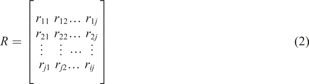
The following illustrates the construction of the correlation coefficient matrix by calculating the correlation coefficient between the explanatory variable and explained variable
According to the initial correlation coefficient matrix, the partial regression sum of squares between different explanatory variables and explained variable is calculated, which characterize the contribution of different explanatory variables.
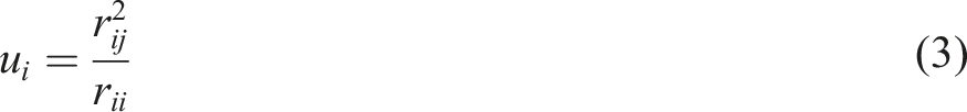
The explanatory variable corresponding to the maximum partial regression square and is selected as the introduced variable and is analyzed by the F-test. When the test result is greater than the empirically determined critical threshold, the variable can be introduced into the regression equation as the regression variable. Otherwise, the variable cannot be introduced into the regression equation and thus needs to be eliminated.
After the variable is successfully introduced, it needs to be used as the main element. The contribution of the variable is eliminated by solving the inverse compact transformation method, and a new correlation coefficient matrix is calculated. The partial regression sum of squares of each explanatory variable is recalculated using the new correlation coefficient matrix. This is performed to find the contribution of the remaining variables and then determine the newly introduced regression equation variables via the F-test until the regression equation cannot introduce or eliminate any variables. At this time, the selected explanatory variable is the introduced independent variable of the regression equation.
After selecting the explanatory variable, the regression coefficient corresponding to each variable can be calculated using equation (4), with the regression coefficient of the unselected variables being 0.

Where
First-order difference method
The first-order difference method refers to the difference between two consecutive adjacent items in a discrete function. The first-order difference demonstrates the magnitude of change of the dependent variable y (Soon-Mo and Woo, 2016). Supposing the function y = f(x), where y is only defined on the non-negative integer value of x and the independent variable x is taken over by non-negative integers in turn, that is, when x = 0, 1, 2, 3, ..., the corresponding function value is

Abbreviated as

When the independent variable changes from x to x+1, the change in the function y = y(x) is as follows

The above equation is called the first difference of the function y(x) at point x, usually written as

Spatial econometric model
Spatial weights matrix
The spatial weights matrix plays a significant role in the spatial econometric model; it is the simplest and most commonly used method for influencing spatial interaction. There are two criteria for its construction: one is to consider the relationship between the geographic spaces, and the other is to consider the economic relationship between regions (Bavaud, 1998). Among them, the spatial weights matrix that considers the relationship between the geographic spaces includes the matrix based on the adjacency relationship (divided into the rook adjacency matrix and queen adjacency matrix) and the matrix based on the physical distance (divided into the k-nearest neighbor spatial weight and threshold weight matrix). The matrix considering the economic relations between regions is the spatial weights matrix based on economic distance (Ying, 2000). Based on the purpose of this paper, the k-nearest neighbor spatial weight matrix is adopted.
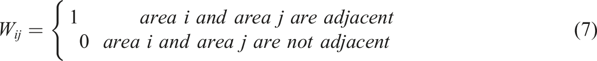
First, we need to set a threshold k and calculate the distances between area i and other areas. Then, we select k areas closest to the area i from them. We believe that these areas and area i are adjacent; they are assigned a value of 1. The remaining areas are not adjacent to area i and are assigned a value of 0.
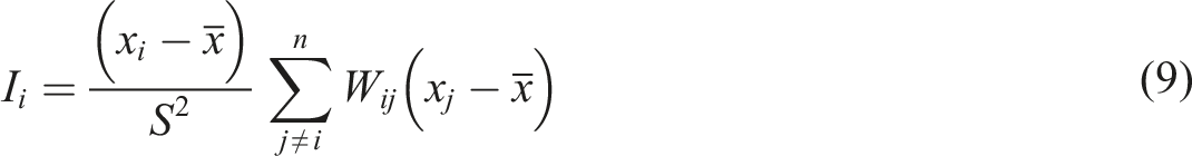
Moran’s I
The first law of geography states that a correlation is present between things—the closer the distance, the stronger the correlation, and the farther the distance, the weaker the correlation. The main methods for testing a spatial correlation are Moran’s I, G statistical test, Geary coefficient, LR (likelihood ratio) test, Wald test, spatial error Lagrangian multiplier (LMerr), and spatial lag Lagrangian multiplier (LMlag) (Jong et al., 2010). Among these methods, the most popular among scholars is Moran’s I, which is divided into global Moran’s I and local Moran’s I to measure the similarity of the attribute values of an object in adjacent regions of space (Ying, 2000). The equation of global Moran’s I is as follows
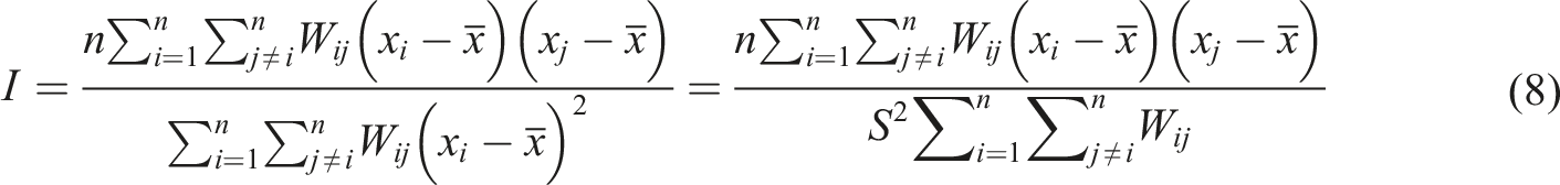
Where I denotes the Moran index:
The equation of local Moran’s I is as follows
Spatial econometrics panel data model
For most of the prior studies using the ordinary econometric regression method (Bond et al., 2001; Klette and Griliches, 1996), there might be bias and inconsistency in the estimative results if the endogenous issues between variables were ignored. In other words, endogenous issues consist of reverse causality, omitted variables, and measuring error. However, for other previous studies using spatial econometric models, these endogenous issues between variables can be better avoided (Lesage, 2008; Yang et al., 2017). In particular, in our paper, we first chose some independent variables based on stepwise regression and then instigated factors affecting tourism flows using the spatial econometric models. In fact, facing the possible endogenous issues in the spatial econometric models, Lesage (2008) pointed out in Chapter 2 and 3 of her book named Introduction to Spatial Econometrics that ordinary OLS estimation magnifies the traditional omission bias and uses spatial econometric models such as SDM and consistent estimators can obtain estimates that are not magnified biases. In addition, the spatial econometric model adopts maximum likelihood estimation, which can reduce the endogenous problem (Anselin, 2003). Yang and Fik (2014) also pointed out that the possible endogeneity problem can be alleviated by using spatial econometric models in their study.
The spatial econometrics model is developed on the basis of ordinary econometrics. A main assumption of the ordinary econometrics model is that each observation is independent, while the assumption of the spatial econometrics model is that the observations are spatially related. Spatial correlation means that observations at different locations are not independent in space, but present a certain non-random spatial pattern, that is y i = f(y i ). i = 1, 2, …, n, i≠j. If the distribution of observations in adjacent areas is similar, it indicates that there is a positive spatial autocorrelation, and if there is no similarity, it indicates that there is a negative spatial autocorrelation, if the distribution of observations in adjacent areas does not have a regular pattern, it indicates that there is no spatial correlation (in spatial data analysis, Moran’s I is generally used to measure the correlation of spatial data). The spatial effect determines that the analysis of spatial data can no longer continue to use the previous analysis method of OLS regression.
In general, the spatial econometrics model includes the spatial Durbin model (SDM), spatial lag model (SLM), and spatial error model (SEM). SDM measures whether variables have spillover effects in adjacent areas. This model indicates that the surrounding areas affect not only the explained variables but also the explanatory variables. The model can be expressed as follows

The SDM model can be estimated by the maximum likelihood estimation (MLE), and its log-likelihood function is specified as follows (Anselin, 2003)
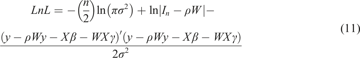
For computational convenience, the log-likelihood can be concentrated with respect to the coefficients
If

Spatial lag model discusses whether the variables have spillover effects in adjacent regions. It mainly examines the spatial correlation of variables in various regions (Anselin, 2003) and indicates that the explained variables are affected not only by various local factors but also by the explained variables in neighboring areas. The meaning of each variable of the above equation is presented in equation (10). The SLM model was also estimated by the MLE method.
If

The spatial dependence of SEM exists in the error perturbation term, which measures the degree of the error impact influence of the explained variable in the adjacent region on the observed value of the region. It fully considers the impact of spatially related error terms on the explained variable. The meaning of Y, β, and X is presented in equation (10).
For the selection of the best model, first, we employ the spatial Hausman test to determine the fixed-effect (FE) or random-effect (RE) and the maximum-likelihood estimation to estimate the model (Belotti and Ilardi, 2018). Second, we use the Wald test and LR test to determine which among SDM, SEM, and SLM is the best model. If the Wald test and LR test pass the significant test, the SDM will be the best model; If either the Wald test or the LR test fails the significance test, the SLM or SEM is the best. Then, we use the LM lag test, LM error test, Robust-LM lag test, and Robust-LM error test to judge which is the best for SLM and SEM. If the Robust-LM lag test and Robust-LM error test pass the significant test, and LM lag test passes the significant test but the LM error test fails the significant test, the SLM is the best; otherwise, SEM is the best. In the spatial econometric models, the spatial interactions indicate various spatial spillover effects between regions and can be estimated, which is one of the objectives of this research.
Variables and data
The tourism spillover effects can be considered from the perspectives of supply and demand (Yang and Fik, 2014). However, in terms of tourism supply spillover effects, due to the combined effects of various uncertain factors, such as marketing, and productivity in tourism supply, reaching a consensus is difficult on the characterization indicators of such factors, and the feasibility of calculation is low. The factors involved in tourism demand spillover effects are more explicit and direct. Accordingly, we quantitatively investigate the spillover effect of regional tourism cooperation from the perspective of tourism demand.
Summary of variables.
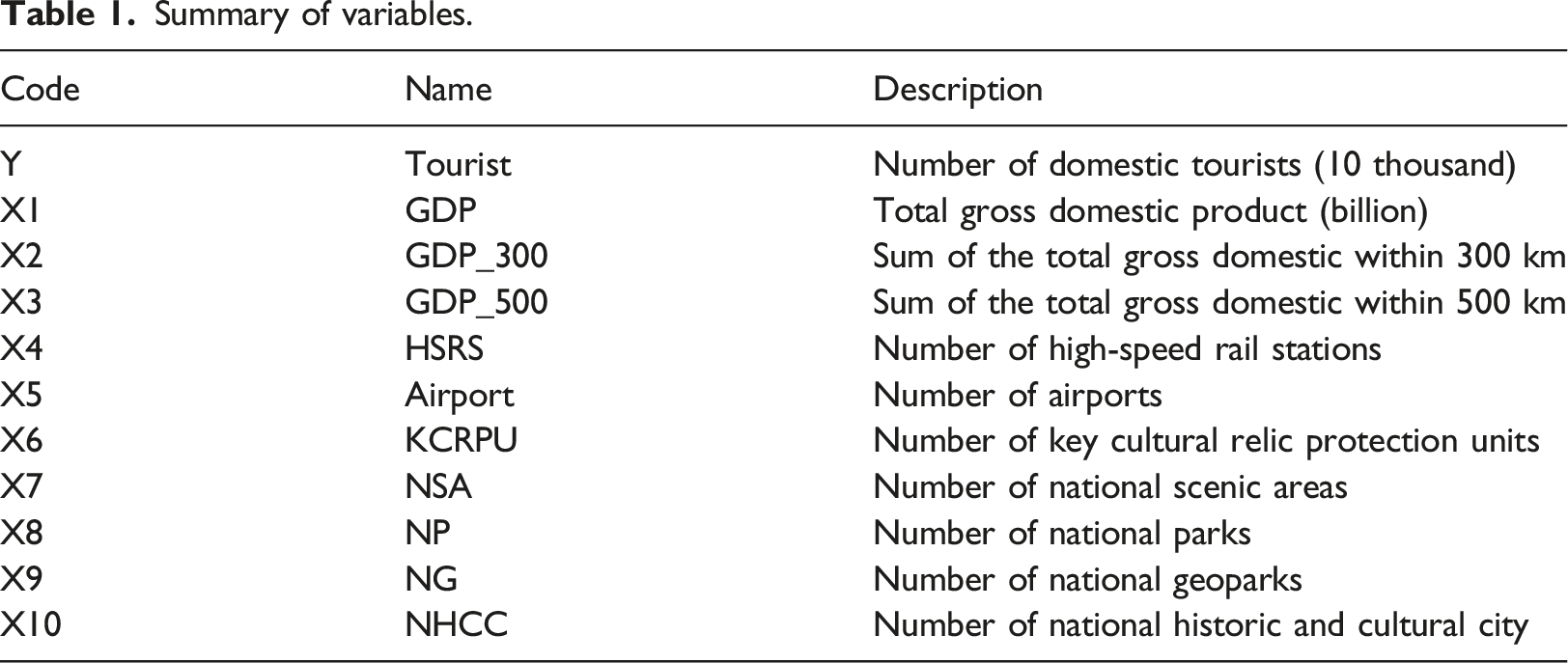
The explained variable Y, tourism demand, is measured as the number of domestic tourists in China (referred to as tourism flows). The number of domestic tourists in China and the domestic tourism income of China are the most popular indicators for tourism demand: 1. X1 represents the level of economic development of each region. 2. X2 and X3 represent the market size in a region. 3. X4 and X5 represent the local traffic accessibility of each prefecture-level city, as well as the strength of the surrounding area and the local traffic connection. The more convenient the traffic, the greater the attraction to tourists. 4. X6–X10 represent the basic tourist attraction of a region and are the first choices of tourists to travel. The number and popularity of tourist attractions in a region strongly influence the development of local tourism. Among them, X6 and X10 represent cultural tourist attractions, whereas X7, X8, and X9 represent natural landscape attractions.
The study period is from 2001 to 2015, and the research data were mainly obtained from the “China Regional Economic Statistical Yearbook,” “China Statistical Yearbook,” and China Scenic Spot website (http://www.chinataa.org). For some areas, if the relevant data cannot be found, we use the growth rate of the area over the years to estimate the missing value of the area in a certain year; in 2011, Anhui province abolished Chaohu City and placed it under the management of Hefei, Wuhu, and Ma’anshan. In this study, the relevant data of Chaohu City were divided into the corresponding regions according to the land area ratio of the three cities for statistics. The research objects are all prefecture-level administrative regions in Mainland China, including prefectures, autonomous prefectures, and leagues, which are all regarded as “city,” among which Chongqing, Shanghai, Tianjin, and Beijing were also deemed as “city” and Hong Kong, Macao, and Taiwan were not considered. Finally, a total of 341 cities were included.
Findings
Descriptive statistics
Descriptive statistics of variables (2001–2015).
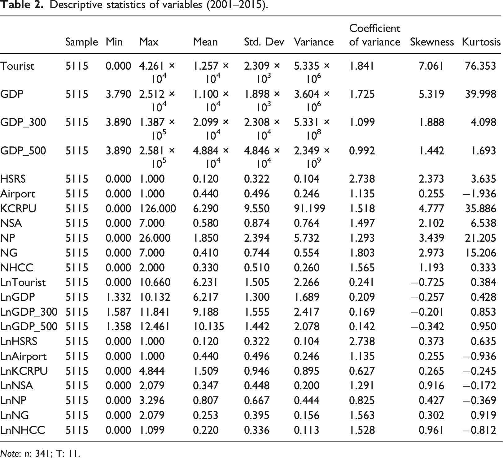
Note: n: 341; T: 11.
From the descriptive statistics of the original data, we can see that the average number of tourists is 1257 million, with the maximum value being 42,606 million and the minimum value being 0. This indicates that the number of domestic tourists is quite different in different cities. Similarly, the Std. Dev of GDP, GDP_300, and GDP_500 are also large, indicating that GDP, GDP_300, and GDP_500 are all fairly different in different cities. This implies that the level of economic development between regions is quite different. The Std. Dev of HSRS and Airport are 0.322 and 0.496, indicating that the difference of HSRS is smaller than that of Airport among regions. KCRPU, NSA, NP, NG, and NHCC all represent tourist attractions, and the differences are also present. Among them, the average value of NSA, NG, and NHCC is less than 1, indicating that the number of NSA, NG, and NHCC is small. The skewness and kurtosis of all these variables are greater than 1, which indicates that the original data does not follow a normal distribution.
From the descriptive statistics of the data after taking the logarithm, we can see that the variance and the coefficient of variance of all variables are smaller than the variance and the coefficient of variance of the original data. And the skewness and kurtosis values of the data after taking the logarithm are less than 1, which means that the data after taking the logarithm is close to a normal distribution. All of these indicated that the data after taking the logarithm is better. Therefore, we use the data after taking the logarithm to analyze the domestic tourism flows. In addition, LnGDP_300 and LnGDP_500 all represent the surrounding market, and these two variables have collinearity to a certain extent. From the variance and coefficient of variance of these two variables, we can see that the variance and coefficient of variance of LnGDP_500 are smaller than LnGDP_300, indicating that LnGDP_500 is better than LnGDP_300. Similarly, LnHSRS and LnAirport all represent the local traffic accessibility of each prefecture-level city, and the variance and coefficient of variance of LnAirport are smaller than LnHSRE, indicating that LnAirport is better. LnKCRPU, LnNSA, LnNP, LnNG, and LnNHCC are all present the basic tourist attraction of a region, and the coefficient of variance of LnKCRPU, LnNSA, and LnNP are smaller than LnNG and LnNHCC.
Selection of optimum explanatory variables
The results of the stepwise regression analysis for 2001–2015.
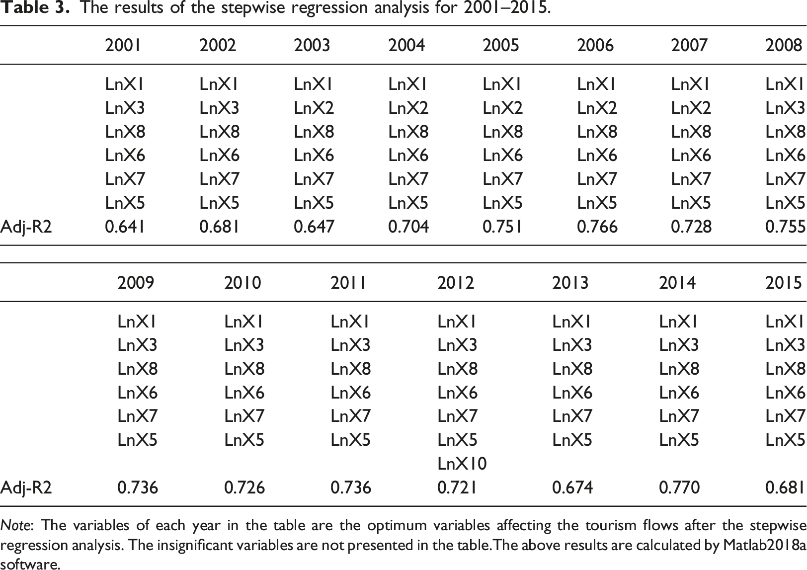
Note: The variables of each year in the table are the optimum variables affecting the tourism flows after the stepwise regression analysis. The insignificant variables are not presented in the table.The above results are calculated by Matlab2018a software.
From the result of the stepwise regression analysis, we can see that LnX1, LnX2, LnX3, LnX5, LnX6, LnX7, LnX8, and LnX10 are the significant variables affecting the tourism flows. LnX2 and LnX3 represent the scale of the tourism demand market in a region; the latter has a significant impact on the tourism flows in 10 of the 15 years, whereas the former has a significant impact on the tourism flows in only 5 of the 15 years. In addition, from the descriptive statistics, we know that the variance and coefficient of variance of LnGDP_500 are smaller than LnGDP_300. Accordingly, we select the LnX3 and delete the LnX2. In addition, a significant impact of LnX10 on the tourism flows is only shown in 2012, and the variance and coefficient of variance of LnX10 are greater than LnX6, LnX7, LnX8, and LnX9; thus, we also delete this variable. Finally, LnX1, LnX3, LnX5, LnX6, LnX7, and LnX8 are selected as the optimum variables affecting tourism flows. And X1 represents the tourism economic fundamental factors, X3 represents surrounding market factors, X5 represents tourism transportation facility factors, and X6, X7, and X8 represent tourist attraction factors.
Spatial correlation of tourism flows
Global Moran’s I
First, we calculate global Moran’s I to examine the global spatial correlation of tourism flows from 2001 to 2015 (Figure 1). From Figure 1, we can determine two particular outcomes: (1) Global Moran’s I of domestic tourists from 2001 to 2015 is greater than zero and thus passes the significant test, indicating that the domestic tourism flows have a positive spatial correlation. This correlation varies depending on the spatial position (distance and space sorting) of things in the geographic space. Many scholars—such as Yang and Fik (2014), Yang and Wang (2014), and Ma et al. (2015)—have asserted that domestic tourism flows have a spatial correlation on different scales. Our research results are consistent with those of previous studies. (2) The overall change trend of Moran’s I from 2001 to 2015 is divided into two stages. The continuous increase from 2001 to 2008 indicates that the spatial agglomeration of domestic tourism flows have increased year by year, that the trend has decreased after 2008, and that global Moran’s I reached the highest level in 2008. Based on the actual circumstances of our country, it can be understood that the grand holding of the 2008 Beijing Olympic Games attracted people from all over the country to migrate to specific areas, thus simultaneously promoting multiregional cross-border activities. The expansion of spatial correlation and agglomeration of tourism flows resulted in global Moran’s I reaching the peak in 2008. Global Moran’s I of domestic tourists in Mainland China during the period of 2001–2015.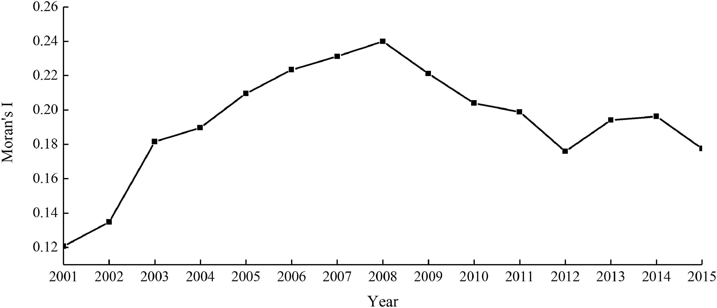
Local Moran’s I
However, global Moran’s I only reflects an average situation. It lacks understanding of the local areas and cannot effectively identify hot spots and cold spots. Therefore, the following part analyzes the spatial correlation of the tourism flows in 2001 and 2015 by using local Moran’s I. From Figure 2, the following can be observed: (1) there are high–high (HH), high–low (HL), low–high (LH), and low–low (LL) agglomeration areas in 2001 and 2015, in which the HH agglomeration indicates that the tourism flows in the region are large, as is the tourism flows in surrounding areas. The HL agglomeration indicates that the tourism flows in this region are larger than those in the surrounding areas. The LH agglomeration indicates that the tourism flows of this area are smaller than those in the surrounding areas. The LL agglomeration indicates that the tourism flows in this area are small, whereas the tourism flows in surrounding areas are also low. The HH and LL agglomerations are concentrated, whereas the HL and LH agglomerations are scattered. (2) From 2001 to 2015, the agglomeration of the tourism flows have undergone significant changes, namely, the scope of HH and LL agglomeration areas has continuously expanded, the number of agglomeration areas has been increasing, the number of HL and LH agglomeration areas has been decreasing, and the scope of LL agglomeration areas has slightly changed. (3) The HH agglomeration areas in 2001 were mainly distributed in the eastern coastal areas, such as the Beijing–Tianjin–Tangshan area, the Shandong Peninsula, the Yangtze River Delta, and the Pearl River Delta. These have been the priority development areas in China after the implementation of the reform and opening-up policy. Various preferential policies are provided, the level of economic development is relatively high, and the domestic and international connections are relatively large. Therefore, the tourism industry was developed across the country to form the HH agglomeration areas. By 2015, the HH cluster areas were not only limited to the eastern coastal areas; these areas included the central regions, such as the Shanxi Province, Sichuan Province, and Guizhou Province. The main reason for this change is that regional tourism cooperation has developed China’s tourism, and the LL agglomeration areas are mainly distributed in the northwest and northeast of China. Since ancient times, the northwest region, which has a large area and sparse population, has been at a low level of economic development in China. Although this region is rich in tourism resources, it has not been well developed. Therefore, its level of tourism development is relatively low. By 2015, the northwest region remains to be in the LL cluster area. The LISA agglomeration diagram of domestic tourism flows in China in (a) 2001 and (b) 2015.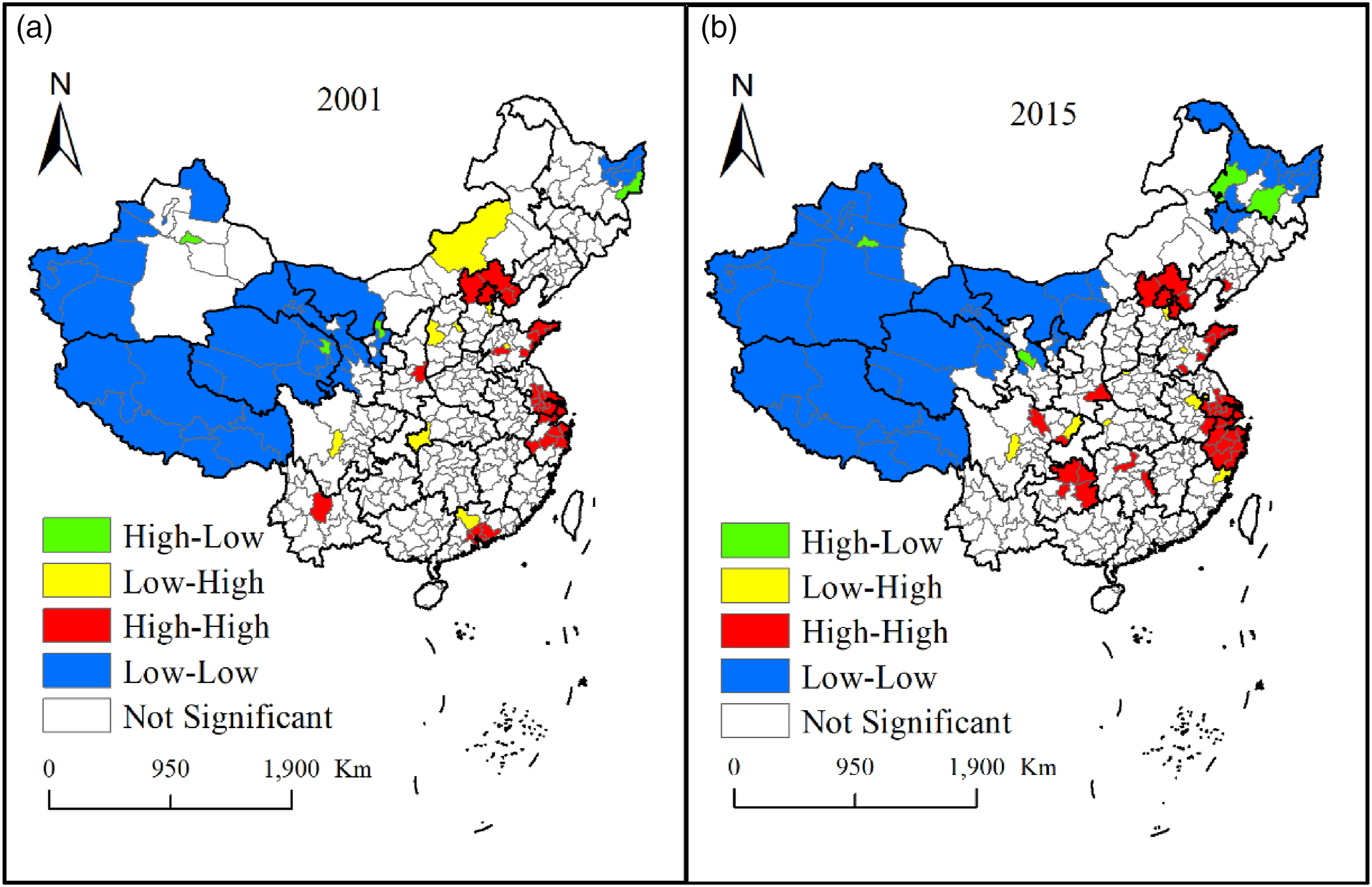
The optimum size of regional tourism cooperation and regional differences
Selecting the best spatial econometric model
The Wald test and LR test.
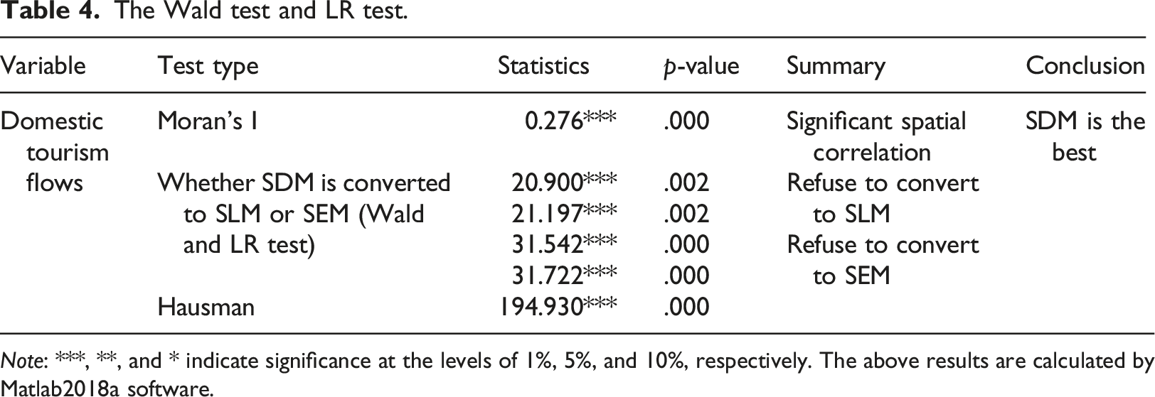
Note: ***, **, and * indicate significance at the levels of 1%, 5%, and 10%, respectively. The above results are calculated by Matlab2018a software.
The regression results of three kinds of fixed-effects SDM (k = 4).
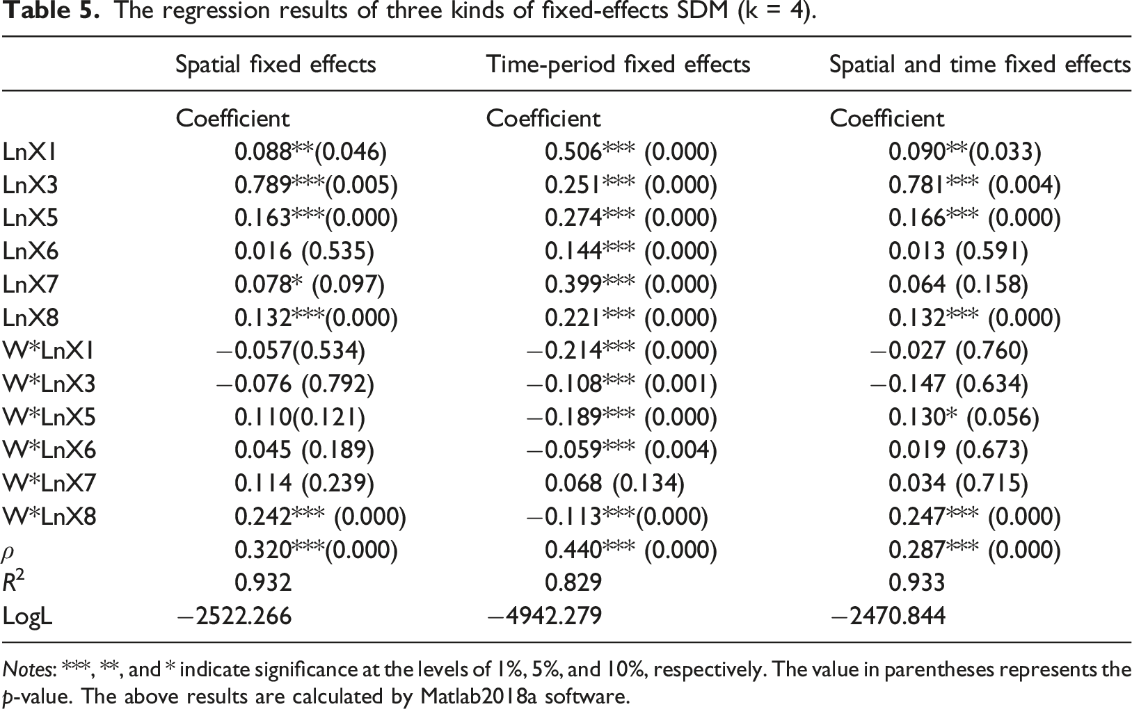
Notes: ***, **, and * indicate significance at the levels of 1%, 5%, and 10%, respectively. The value in parentheses represents the p-value. The above results are calculated by Matlab2018a software.
The SDM (spatial and time fixed effects) results under different k-nearest neighbor spatial weight matrices.
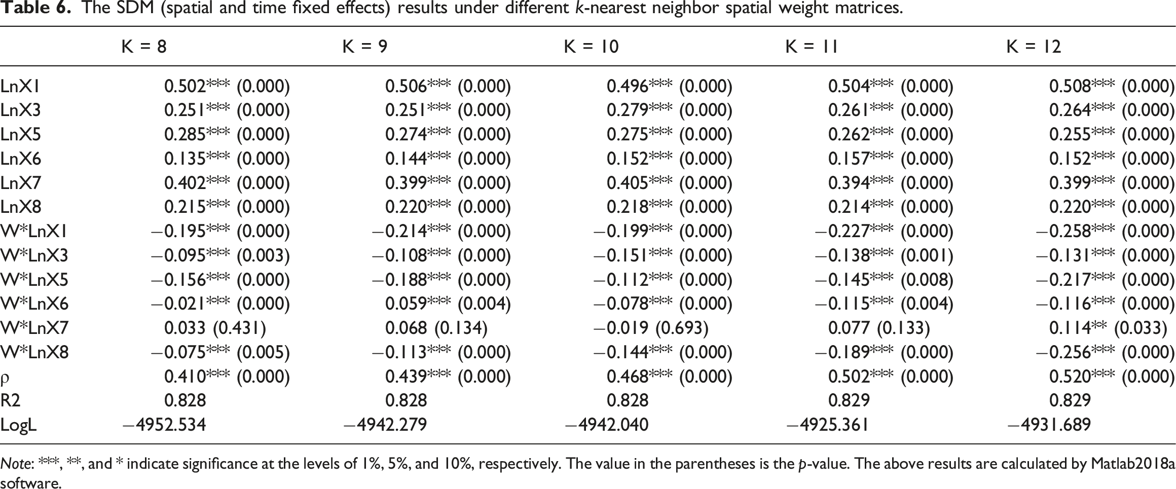
Note: ***, **, and * indicate significance at the levels of 1%, 5%, and 10%, respectively. The value in the parentheses is the p-value. The above results are calculated by Matlab2018a software.
The optimum scale of regional tourism cooperation in Mainland China
At present, more than 40 regional tourism cooperations exist in Mainland China. The scales of the cooperation are different, and there is no standard scale of the regional tourism cooperation. After analyzing all these regional tourism cooperation, most of the cities included in single regional tourism cooperation are found to be 4, followed by 7 or 8, and the number of cities included in some regional tourism cooperation even reaches 17, 19, and 25 (Figure 3). However, how to determine the scale of these regional tourism cooperation and whether the scale of the regional tourism cooperation is reasonable? Previous scholars lacked the quantitative explanation. Therefore, research on the optimum scale of regional tourism cooperation requires further work. The frequency distribution map of the number of cities in single regional tourism cooperation.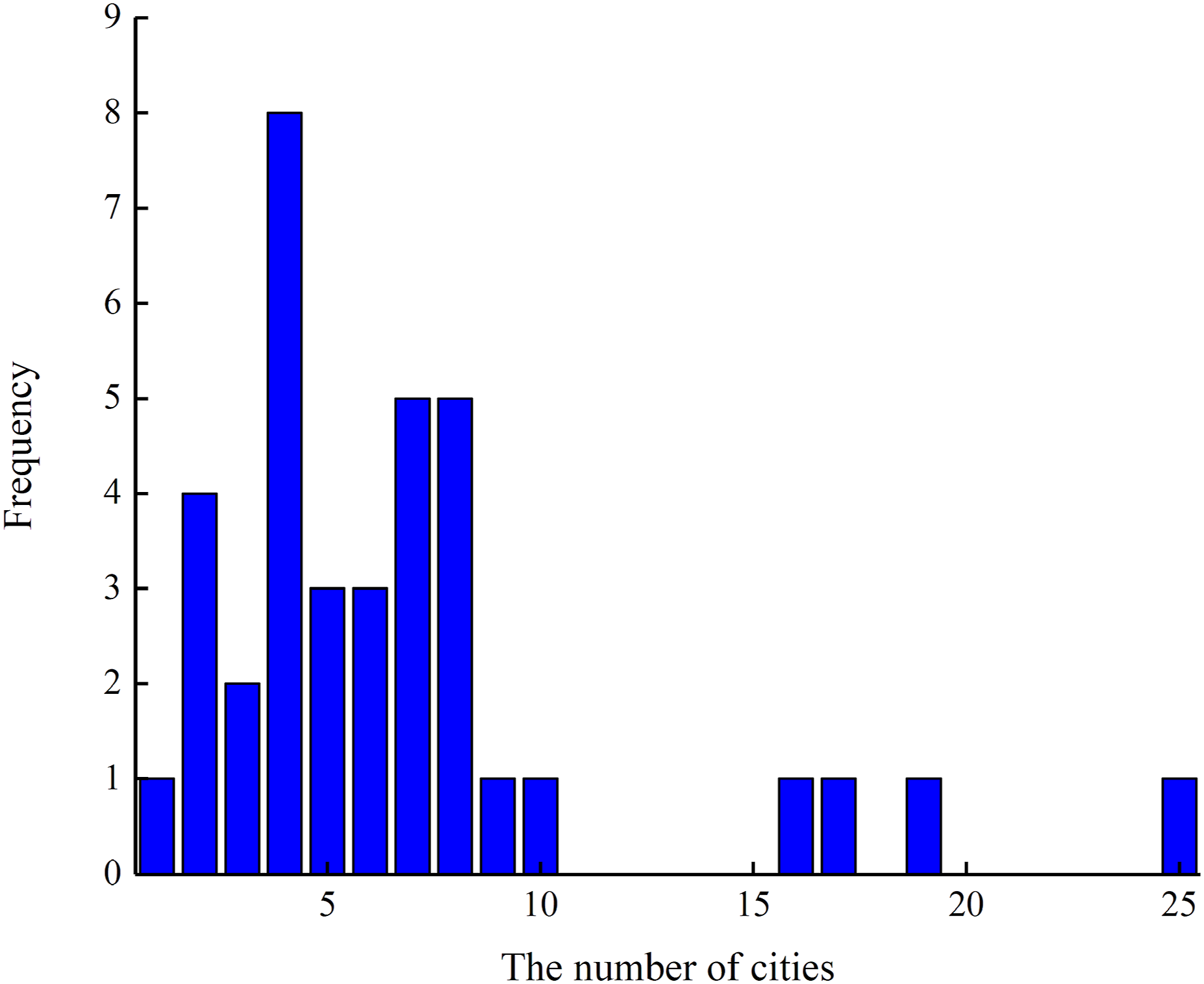
Based on Figure 3, this study set 50 k-nearest neighbor spatial weight matrices, and the values of k in the k-nearest neighbor spatial weight matrices are taken from 1 to 50, respectively. The main reason is that in previous studies, the number of cities in Mainland China for regional tourism cooperation was up to 25. Moreover, there cannot be too many cities for regional tourism cooperation as it will result in the waste of resources, which is not conducive to the maximization of tourism benefits. Therefore, we set here the upper limit of k as 50. Then, the 50 k-nearest neighbor spatial weight matrices are sequentially brought into the SDM to discuss the tourism flows spillover coefficient. In the process of spillover coefficient analysis, we introduce the first-order difference method to judge the stability of the tourism flows spillover coefficient.
Figure 4(a) presents the change in the tourism flows spillover coefficient in all cities in Mainland China with the increase in the number of adjacent cities. From the figure, it can be seen that the change trend first exhibits a rapid increase, followed by a slow increase, with a certain degree of stability. Moreover, the spillover coefficient is negative when k = 1, k = 2, and k = 3, indicating that when the number of cities included in regional tourism cooperation is not more than four, the tourism development between cities is in a state of competition, and regional tourism cooperation is not conducive to the development of cities. The central concept of this paper is to identify the optimum scale of regional tourism cooperation according to the changes in the spillover coefficient of tourism flows. Although it can be seen from Figure 4(a) that the tourism flows spillover coefficient is exhibiting an upward trend overall, we cannot induce that having a greater number of cities joining in building regional tourism cooperation is better. If the number of cities is large, the cost of cooperation between regions will increase, and the coordination of various issues will also decline, which is not conducive to the smooth development of regional tourism cooperation. Accordingly, we believe that when the tourism flows spillover coefficient exhibits a shift from rapid growth to slow growth, the range of k is the optimum scale of the regional tourism cooperation. For Mainland China, it can be seen from Figure 4(b) that when k = 4, the variation range of the tourism flows spillover coefficient becomes smaller. Figure 4(a) demonstrates that when k = 4, the tourism flows spillover coefficient reaches a higher value than when k = 1, k = 2, and k = 3. When k = 14, the spillover coefficient reaches a peak, and the variation range of the spillover coefficient begins to stabilize. From Figure 4(b), it can be seen that with the increase in the number of cities, the change trend of the tourism flows spillover coefficient begins to stabilize, especially when k = 14. This indicates that with the continuous increase in the number of cities, the tourism flows spillover coefficient does not significantly change, and when the value of the k-nearest neighbors reaches more than 14, the tourism cooperation between cities will not have a strong advantage. Therefore, we believe that when the number of the k-nearest neighbors’ cities are [4, 14], that is, when the number of cities that constitute regional tourism cooperation is [5, 15], the scale of regional tourism cooperation is reasonable. Global Moran’s I of domestic tourists in Mainland China during the period of 2001–2015.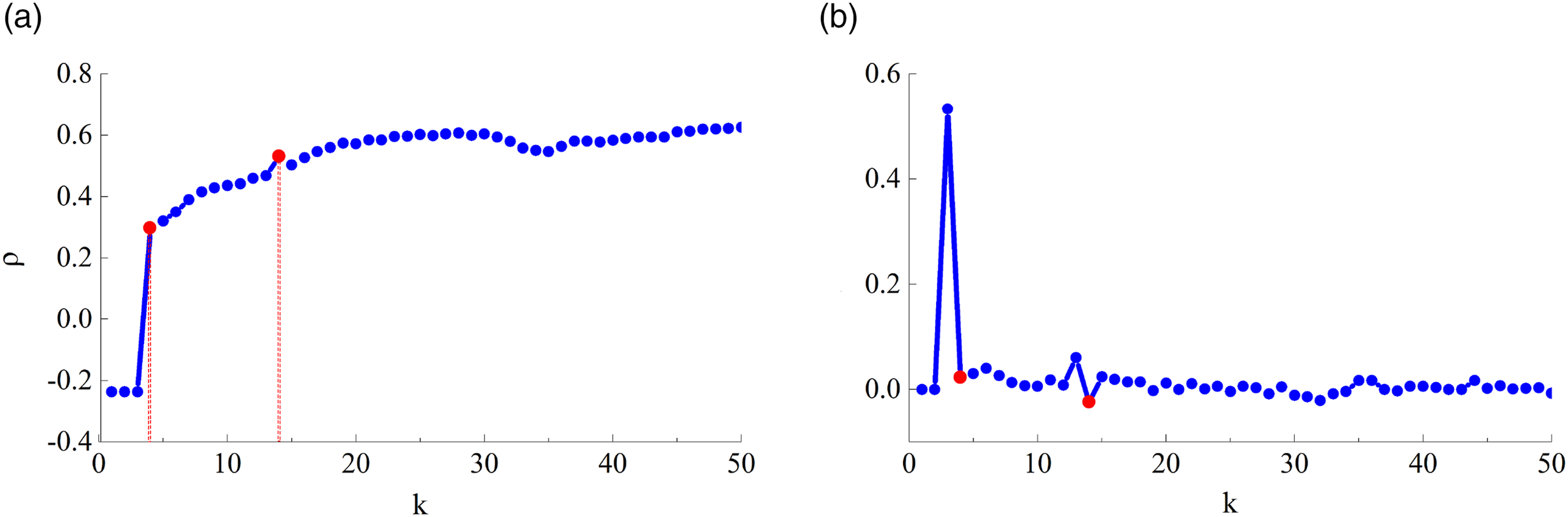
Regional differences in the optimum scale of regional tourism cooperation
Due to the expansion of China’s territory and the large regional differences, different regions have different scales when constructing regional tourism cooperation. To further analyze the differences in the scale of regional tourism cooperation in the different regions of China, we use China’s three major economic zones (http://news.xinhuanet.com) as the dividing standard to divide China into the eastern region and the midwestern region. The eastern part includes 130 cities in 12 provinces, including Beijing, Tianjin, Liaoning, Hebei, Shandong, Jiangsu Sheng, Shanghai, Zhejiang, Fujian, Guangdong, Guangxi, and Hainan. The midwestern part encompasses 228 cities in other provinces, except the eastern part. Analogously, for the eastern region and the midwestern region, we also constructed 50 k-nearest neighbor spatial weight matrices, where the value of k is 1–50, and they are, respectively, brought into the SDM to extract the spillover coefficient so that the differences in different regions can be analyzed. Figures 5 and 6 present the changes in the tourism flows spillover coefficient in the eastern and midwestern regions. The tourism spillover coefficient under different k-nearest neighbor spatial weight matrices in (a) eastern China and (b) its first-order difference result. The tourism spillover coefficient under different k-nearest neighbor spatial weight matrices in (a) midwestern China and (b) its first-order difference result.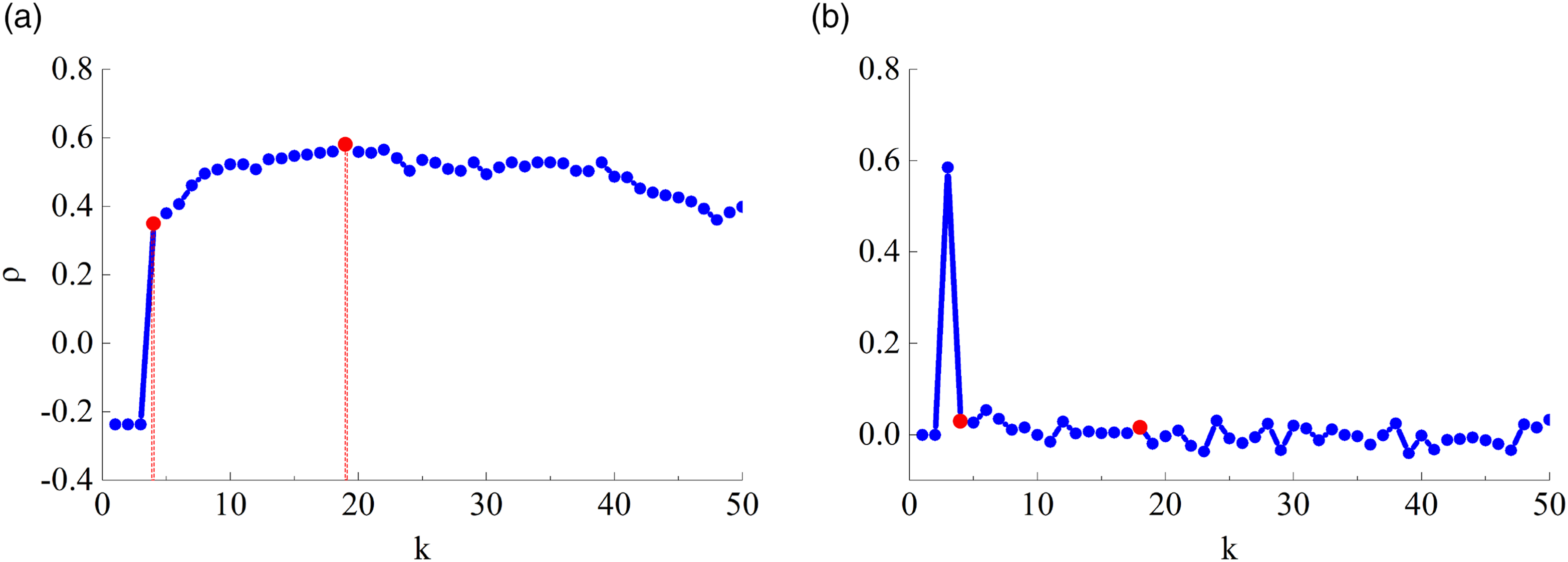
The spillover coefficient in the eastern region initially demonstrated a rapid increase, followed by a slow increase to a high value and then a slow decrease (Figure 5(a)). When the value of k is 4, the tourism flows spillover coefficient evidently shifts from being negative to positive, and as the value of k continues to increase, the tourism flows coefficient also continues to increase. When the value of k is 19, the tourism flows spillover coefficient reaches its maximum. When the value of k is between 20 and 50, the tourism flows spillover coefficient exhibits a downward trend, which indicates that when the number of cities is within the range of [20, 50], the overall benefits of the regional tourism cooperation continuously decrease. The regional tourism cooperation constructed at this time violated the principle of win–win cooperation, rendering it unsuitable for building large-scale regional tourism cooperation. The main reason for this is that the tourism industry in the eastern region is relatively developed, and the tourism cooperation between regions is relatively mature, which has reached the phenomenon of increasing returns to scale. With the increase in the number of cities, tourism cooperation between regions is expected to gradually reach saturation. Exceeding a certain range will destroy the balance between regions and reduce the overall benefits. Figure 5(b) also demonstrates that the change trend of the spillover coefficient is stable when k is between 4 and 19. And when k is between 20 and 50, the change trend of the spillover coefficient is also stable. Therefore, we believe that the number of cities needed to achieve an optimum regional tourism cooperation in the eastern region is [5, 20].
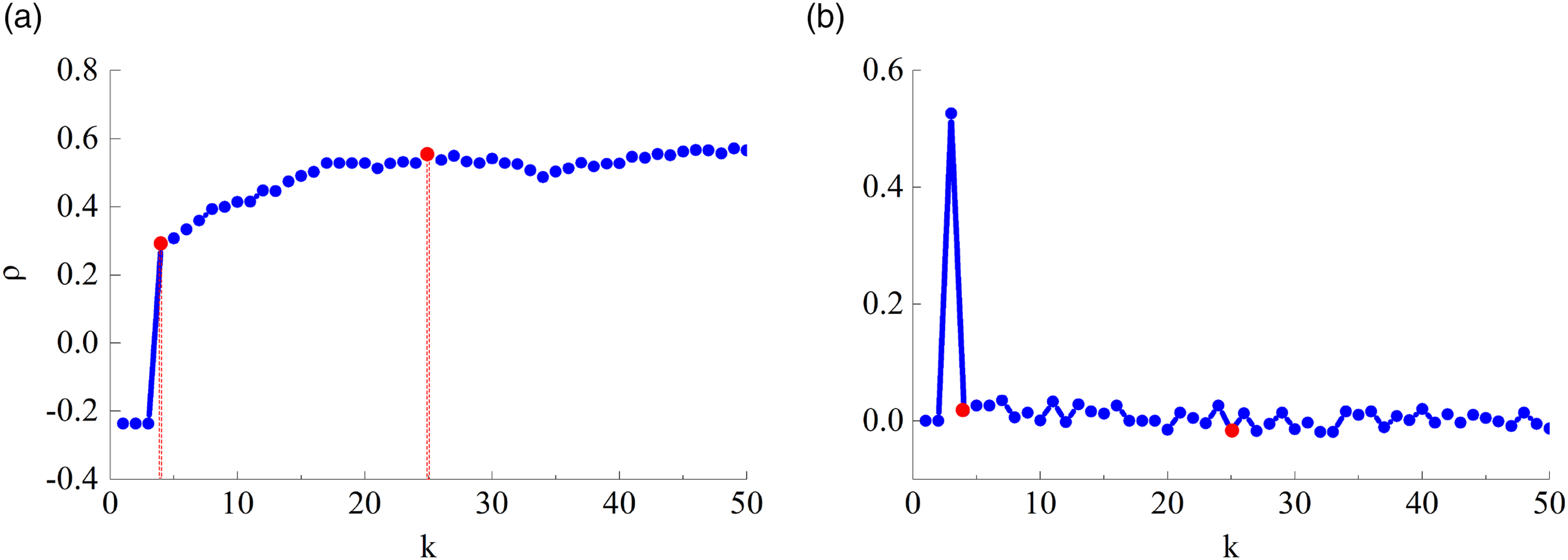
Midwestern China exhibits a change trend of its tourism flows spillover coefficient similar to Mainland China: it first demonstrates an increasing trend, followed by a decreasing and a slowly increasing trend (Figure 6(a)). Similarly, for the midwestern region, we believe that the turning point when the change trend of tourism flows spillover coefficient shifts from rapidly increasing to slowly increasing is the optimum number of cities for building regional tourism cooperation. From Figure 6(a), it can be seen that when k = 4, it is evident that the coefficient of tourism flows spillover shifts from negative to positive. When k = 25, the coefficient of tourism flows spillover reaches a high value and then starts to decrease. In addition, when k = 35, the tourism flows spillover coefficient starts to increase again, and the number of cities in the regional tourism cooperation reaches 50 when the spillover coefficient again reaches the same level as the k = 25. The participation of a large number of cities will result in a waste of tourism resources, which is not conducive to the healthy development of the regional tourism cooperation. From Figure 6(b), it can be seen that the change trend of the spillover coefficient is stable after k = 25 in the k-nearest neighbor spatial weight matrix. Therefore, we believe that when the value range of k is between 4 and 25, the scale of the regional tourism cooperation is optimum. Therefore, the number of optimum cities in the midwestern region that constitute the regional tourism cooperation is [5, 26].
After comparing and analyzing the differences between the eastern and midwestern regions, we also compare the differences between the northern and southern regions. The southern region mainly includes Shanghai and all cities in Zhejiang Province, Jiangsu Province, Jiangxi Province, Anhui Province, Hunan Province, Hubei Province, Chongqing Province, Sichuan Province, Yunnan Province, Guizhou Province, Guangxi Province, Fujian Province, Guangdong Province, and Hainan Province. The northern region mainly consists of Beijing, Tianjin, and all cities in Shandong Province, Henan Province, Shanxi Province, Shanxi Province, Hebei Province, Gansu Province, Qinghai Province, Xinjiang Uygur Autonomous Region, Inner Mongolia Autonomous Region, Liaoning Province, Jilin Province, and Heilongjiang Province. The cities in the Tibet Autonomous Region are not considered as the region is not suitable for the development of regional tourism cooperation due to its roundabout area, harsh environment, relatively scattered tourism resources, and few high-level tourism resources. Similarly, 50 k-nearest neighbor spatial weight matrices were selected to calculate the tourism flows spillover coefficient. The results are presented in Figures 7 and 8. The tourism spillover coefficient under different k-nearest neighbor spatial weight matrices in (a) northern China and (b) its first-order difference result. The tourism spillover coefficient under different k-nearest neighbor spatial weight matrices in (a) southern China and (b) its first-order difference result.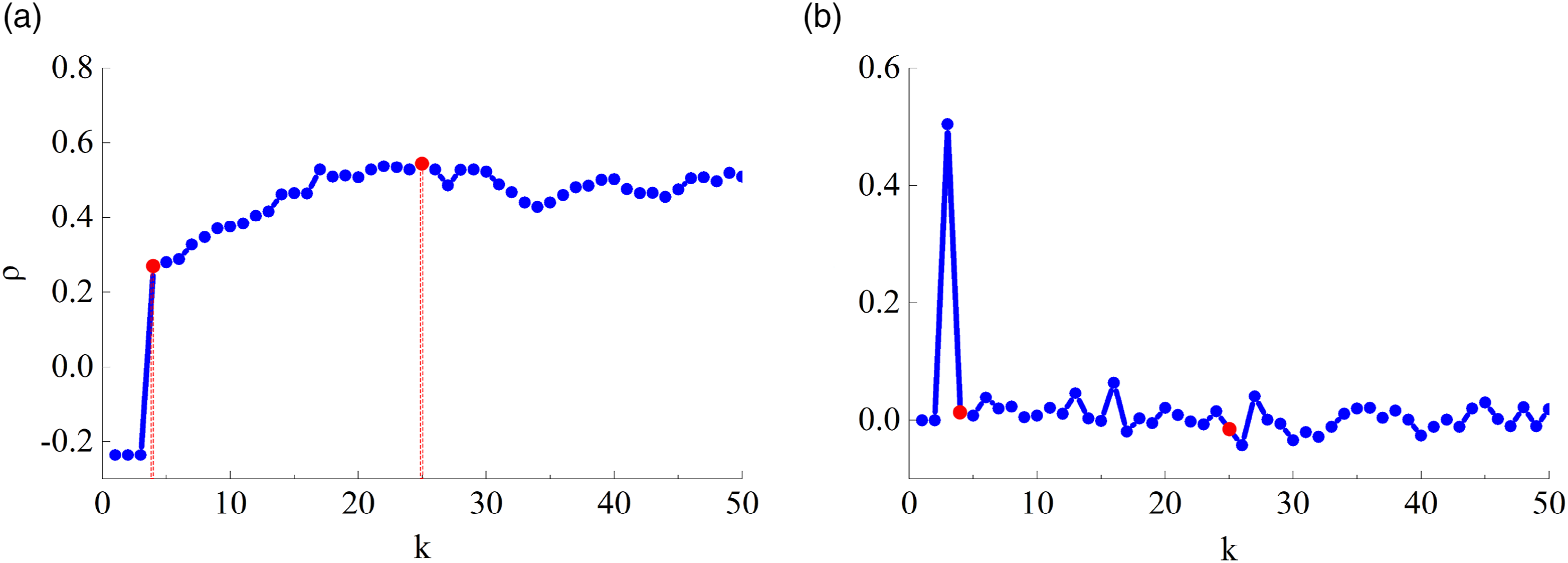
As can be seen from Figure 7(a), the tourism flows spillover coefficient in the northern region initially exhibits a rapidly increasing trend, followed by a slowly increasing trend. When k = 25, the tourism flows spillover coefficient reaches the maximum value, which is 0.57, and thus passes the significance test at the level of 1%, indicating that every 1% increase in the number of tourists from neighboring areas will result in an increase of 0.57% in the number of tourists in that area. The spatial effect of tourism flows between regions is mainly reflected by the spatial effect of neighboring regions. However, this spillover effect of tourism flows does not always increase with the increase in the number of neighboring cities. However, a bottleneck period appears in the process of a gradual increase in the number of neighboring cities, causing the elasticity of tourism flows to decrease. According to Wang and Wang’s (2000) explanation of the location theory of the tourism industry, when the marginal utility is greater than 1, tourists will be attracted to the destination. When the marginal utility is less than 1, even if the destination has abundant tourism resources, it will not attract more tourists. Therefore, in the interval of k = 25 and k = 34, the marginal utility of tourists from surrounding areas to a certain destination decreases. Thus, the tourism spillover coefficient decreases. However, as the value of k increases, the marginal utility of tourists exhibits an increasing trend. The regional tourism cooperation shows the development stage, the bottleneck stage, and the consolidation stage. In constructing regional tourism cooperation, not only the tourism marginal utility of tourists needs to be considered but also other factors. Based on Figure 7(a) and Figure 7(b), we believe that the optimum number of cities for constructing the regional tourism cooperation is between 5 and 26 in the northern region.
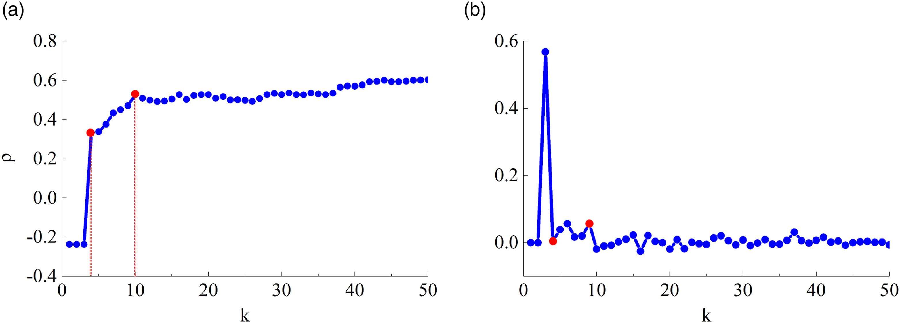
Figure 8(a) presents the changes in the tourism flows spillover coefficient in the southern region. The difference between the northern region and southern region is that the latter exhibits a rapidly increasing trend, followed by a slightly decreasing and then a slowly increasing trend, which is not as obvious as in the northern region. When k = 10, the tourism flows spillover coefficient reaches the first peak value. Figure 8(b) presents the result of the first-order difference; from the figure, it can be seen that when the value of k is greater than 10, the change trend of the tourism flows spillover coefficient is relatively stable. Hence, we believe that the optimum number of cities for constructing regional tourism cooperation is [5, 11]. The optimum scale of the northern and southern regional tourism cooperation exhibits a relatively large difference. Probably, the main reason is that tourism in the northern region mostly pertains to sightseeing, and only by connecting multiple cities can the benefits of regional cooperation be maximized. However, the southern regions mostly involve vacation tourism, and the destinations are relatively independent. When constructing regional tourism cooperation, only a small number of cities can be added to maximize the spillover between regions.
The stability of tourism flows spillover and optimum regional tourism cooperation
Based on the changes in the tourism flows spillover coefficients across Mainland China—eastern region, midwestern region, northern region, and southern region—the differences of the different regions can be observed: the optimum number of cities for constructing regional tourism cooperation in Mainland China is [5, 15], the ideal number of cities within the cooperation in the eastern region is [5, 20], the most favorable number of cities in the midwestern region is [5, 26], the most advantageous number of cities in the northern region is [5, 26], and the optimum number of cities in regional tourism cooperation in the southern region is [5, 11]. All of these indicate that the different regions are divided, and the optimum scale of the regional tourism cooperation is also different due to the different cities joining the cooperation. The reason for the difference in the scale of the eastern and midwestern regional tourism cooperation is mainly because the development of tourism in the eastern region is more mature than that in the midwestern region. Moreover, adding only a small number of cities to the cooperation can lead to the optimization of the overall benefits of the region. For the midwestern region, the development of the cooperation is not yet mature, and the expansion or reduction of the scale impacts the overall benefits of the region. Therefore, the scale of the regional tourism cooperation in the midwestern regions has stabilized near a fixed value. With continuous development, the optimum scale of cooperation will change. A substantial difference can be observed in the optimum size of the regional tourism cooperation between the northern and southern regions, mainly because the people in these regions have different needs for tourism: the north mainly desires sightseeing, whereas the south desires holiday tourism.
Conclusion
This paper takes the domestic tourism flows of 341 cities in Mainland China as the research object and discusses the optimum scale of regional tourism cooperation from the perspective of the spatial spillover effect of tourism flows and the k-nearest spatial weight matrix by using spatial econometric methods. Compared with the previous studies, the research features of this article are mainly manifested in the following aspects: first, 341 cities in Mainland China are the research objects, thus covering an extensive area and involving numerous cities; second, from the perspective of geospatial correlation, global Moran’s I and local Moran’s I of domestic tourism flows are employed to prove whether the tourism flows is spatially relevant; third, on the basis of judging the spatial correlation, the spatial econometric model is used to determine the reasons for the spillover effect between tourism flows; and finally, by constructing and using the k-nearest neighbor spatial weight matrix, setting different values for k, observing the change trend of tourism flows spillover effects under different spatial weighting matrices, and combining the actual situation, the optimum scale of regional tourism cooperation in Mainland China and different regions was analyzed and determined. The main conclusions are as follows: (1) The tourism economic fundamental factor, surrounding market factor, tourism transportation facility factor, and tourist attraction factors all have a positive and significant impact not only on local tourism flows but also on the surrounding areas, with tourism economic fundamental factor having the greatest impact. Based on previous studies, this paper summarizes 10 factors as explanatory variables that influence tourism flows. By using the stepwise regression, six significant factors were finally obtained, and GDP represents the tourism economic fundamental factor, GDP_500 represents surrounding market factor, Airport represents tourism transportation facility factor, and KCRPU, NSA, and NP represent tourist attraction factors, indicating that these are currently the most important factors affecting domestic tourism flows. Furthermore, we found that these factors also had a significant impact on the tourists in the surrounding areas. (2) A spatial correlation exists in the tourism flows between regions, and it gradually increases over time. Spatial correlation promotes the spillover effects of tourism flows between different regions, which is the basis for regional tourism cooperation. (3) The optimum scale of regional tourism cooperation in Mainland China and the different regions is presented. The optimum number of cities of the regional tourism cooperation in Mainland China is [5, 15], the ideal number of cities of the cooperation in the eastern region is [5, 20], the most favorable number of cities in the central and western regions is [5, 26], the most advantageous number of cities in the northern region is [5, 26], and the optimum number of cities of regional tourism cooperation in the southern region is [5, 11].
In order to further explore the optimal scale of regional tourism cooperation, we analyze and summarize the shortcomings in previous studies and use the spatial econometric model to explore from the perspective of the spatial weight matrix. The stepwise regression is used to extract explanatory variables to make the factors that affect tourism flows more clear. After that, the average scale of regional tourism cooperation across the country and different regions is given. Although compared with previous studies, this paper quantitatively gives the average scale of regional tourism cooperation based on spatial correlation and multi-tourism destinations; there are still some shortcomings that need to be improved.
First, when selecting the spatial weight matrix in this paper, only the k-nearest neighbor spatial weight matrix was considered. In fact, when conduction regional tourism cooperation, the economic development level of a region will also affect whether the region will be included in the regional tourism cooperation. Therefore, in future research, the economic weight matrix should also be taken into consideration. Second, the development of tourism has phases, and the scale of regional tourism cooperation at different stages will be different. This study only considers the overall situation in the past 15 years and does not discuss the phased differences in regional tourism cooperation, which is still an issue worthy of an in-depth discussion in the future.
Footnotes
Declaration of conflicting interests
The author(s) declared no potential conflicts of interest with respect to the research, authorship, and/or publication of this article.
Funding
The author(s) disclosed receipt of the following financial support for the research, authorship, and/or publication of this article:This work was supported by the (Fundamental Research Funds for the Central Universities) under Grant number (2021ECNU-HWCBFBLW009) and the [National Natural Science Foundation of China] under Grant (number 42130510).