
Abstract
Forecasting tourism demand in a timely manner is critical for ensuring the smooth operation of the tourism industry. Over time, time series models have been widely applied to estimate the number of tourists arriving. In this paper, we proposed a XGBoost model for tourism demand forecasting based on the STL seasonal decomposition. The first phase of our proposed model involves applying STL decomposition to preprocess the time series, separating it into two components: the seasonal and de-seasonal terms. During the second phase, the seasonal term is modeled and predicted with the Holt-Winters model. For the de-seasonal term, the ARIMA model is first employed to capture the residual part, Then, the XGBoost model is utilized to reconstruct both the de-seasonal term and its lag, along with the residual part obtained from the ARIMA model. By integrating the forecast outputs from both the Holt-Winters and XGBoost models, the final tourism demand predictions can be derived. The effectiveness of the proposed model is demonstrated using the tourist arrivals data in Macau from eight countries: United States, Germany, Malaysia, Philippines, India, Thailand, Italy and Korea (South Korea). The validation results indicate that the proposed model exhibits superior forecasting performance for time series data showing seasonality and trendency, simultaneously enhancing interpretability without increasing model complexity. The model outperforms five benchmark comparison models when assessed using the Symmetric Mean Absolute Percent Error (SMAPE), Root Mean Square Error (RMSE), Mean Absolute Error (MAE), and Mean Absolute Percentage Error (MAPE) metrics.
Introduction
Tourism demand forecasting research offers valuable insights for governments and businesses, helping them to better anticipate market trends, optimize resource allocation and development, improve tourism service quality, and boost revenue and employment opportunities. Furthermore, accurate forecasting supports the rationalization of marketing strategies and advertising plans to attract more tourists and promote sustainable tourism development.
In research on tourism demand forecasting, its majority of forecasting methods have traditionally focused on time series methods. Many scholars have favored traditional modeling methods for their outstanding explanatory power and simplicity. Commonly used models include ARIMA (Lim and McAleer, 2002), SARIMA (Chang and Liao, 2010), Prophet (Taylor and Letham, 2018), Holt-Winters (Lim and McAleer, 2001), among others.
When utilizing these models to forecast tourist arrivals, only the linear aspect of relevant demand characteristics is taken into consideration. This assumes a linear correlation between future values of the data and the lagged values and residuals. However, when the data exhibits a nonlinear structure, these models may not accurately and precisely forecast. Their effectiveness is prominent when dealing with absence of complex nonlinear components.
For the past few years, various nonlinear methods have been utilized for tourism demand forecasting. These methods can capture the nonlinear structure of tourist data, resulting in a significant enhancement in forecasting accuracy. Currently, the main methods center around support vector machines (Pai et al., 2005), random forests (Zhang and Tang, 2022), gradient boosting trees (Liu et al., 2020), and integrated learning methods such as packing(Athanasopoulos et al., 2018), boosting (Ozaslan et al., 2022) and superposition (Kumar et al., 2022).
Further on, these methods incorporate more complex neural networks for prediction, including Artificial Neural Network (ANN) (Khashei and Bijari, 2010), Convolutional Neural Network (CNN) and Long Short Term Memory Network (LSTM) (Ni et al., 2021), the faster KELM (Sun et al., 2019), and the ensemble deep learning approach(Sun et al., 2022). These models are capable of performing nonlinear and non-stationary forecasting of time series data, significantly enhancing forecasting accuracy.
Despite demonstrating promising accuracy for most time series data, these methods’ performance is highly dependent on the correct selection of hyperparameters, which are typically related to the data. Mis-specification of these parameters can lead to a substantial decrease in forecast accuracy for out-of-sample predictions. Additionally, these complex models are prone to overfitting, meaning they may learn both the underlying patterns and the noise in the data, which can impair their ability to generalize to unseen data. Another significant drawback of some of the approaches mentioned is the lack of interpretability and the “black-box” nature of these models.
On the other hand, to overcome the limitations of single predictive models and enhance their scalability and generalization, researchers have proposed a hybrid of linear and non-linear methods for predicting the tourist arrivals. See next Section for the detailed literature review.
Data decomposition techniques have become a powerful tool in this field due to the unique seasonality and trends in tourist arrival datasets (Zhang et al., 2021). Frequency domain-based decomposition methods have demonstrated superior performance in handling seasonal and nonlinear time series data. Typically, the approach involves decomposing the original data into different components and then applying a combined forecasting strategy. The seasonal component is estimated and removed first, followed by the estimation of the remaining components. Among the standard decomposition methods, X12 (Cuccia and Rizzo, 2011, Empirical Mode Decomposition (EMD) (Fatema et al., 2022), and Seasonal-Trend-Loess (STL) (Gurnani et al., 2017) have been widely used. Researchers (Faraway and Chatfield, 1998; Nelson et al., 1999; Zhang and Qi, 2005) have investigated the effectiveness of time series decomposition, particular de-seasonalization, on modeling and forecasting performance. They found that decompose the time series before applying the models for prediction yields significantly better results, dramatically reduce forecasting errors.
Most studies, including ours, primarily focus on time series decomposition for its specific advantages in interpretability while simultaneously improving the predictive accuracy. In terms of interpretability considerations, these algorithms, encompassing both classic and hybrid methods, typically generate the final aggregate prediction by simply summing up the components. Despite claimed multiple benefits, several remaining issues significantly restrict the further development of these algorithms. Classical models, which assume a linear relationship, are not well-suited to handle complex nonlinear problems. Moreover, the differencing processing employed in these methods often fails to satisfactorily address the nonlinearity and seasonality. Hybrid methods usually combine the seasonal and trend terms using a linear model for forecasting purposes while assuming that only the residual term contains nonlinear factors. However, within the trend term itself- apart from the residual term-there exist not only linear factors but also nonlinear factors. Furthermore, when forecasting with seasonal time series data, incorporating the seasonal component into the forecast together often leads to suboptimal results.
Against the above background, we propose a novel hybrid method for tourism demand forecasting. Specifically, we introduce an XGBoost-based approach that forecasts tourist arrivals using STL seasonal decomposition to address the limitations of existing time series forecasting models. XGBoost, which stands for Extreme Gradient Boosting, is a highly optimized implementation of the gradient boosting algorithm. Its competitive advantage lies in its superior balance between exploration and exploitation, making it more effective than alternative methods. Notably, XGBoost offers key features such as incorporation of diverse regularization penalties to mitigate overfitting risks, and the ability to detect and learn from non-linear data patterns. To extract the seasonal component from the raw data, the Seasonal-Trend-Loess (STL) method is introduced. Compared to other decomposition methods, such as X12 and EMD, STL offers several distinct advantages, including: (1) STL is adaptive to abnormal values which ensures the robustness, thereby enhancing the accuracy of prediction. (2)STL has a wide applicability as it can handle time series with any seasonal frequency greater than one. (3) Being based on numerical methods, STL eliminates the need for parameter determination, making it an easily achievable method.
The application of hybrid models in tourism prediction is still in the stage of continuous exploration. Since the ensemble learning frameworks show promise as an effective method, this study aims to address these gaps by incorporating seasonal decomposition and introducing the interpretable ensemble learning method XGBoost to enhance available datasets and improve prediction performance.
In the first phase of our proposed model, STL decomposition is utilized to preprocess the time series data. This involves decomposing the time series into two components: the seasonal term and the de-seasonal term. During the second phase, we model and predict the seasonal term using the Holt-Winters model. For the de-seasonal term, we first employ the ARIMA model to capture the residual part. Then, the XGBoost model is utilized to reconstruct both the de-seasonal term and its lag, along with the residual part obtained from the ARIMA model. By combining the forecast results from the Holt-Winters model and the XGBoost model, we can obtain the final forecasting tourist arrivals. Furthermore, a direct strategy is used to implement multi-step-ahead forecasts.
The remainder of the paper is organized as follows. Section 2 provides a review of the literature on the forecasting of tourism demand using hybrid methods. Section 3 provides a brief overview of the basic modeling approaches, including Seasonal-Trend-Loess (STL), Auto-Regressive Integrated Moving Average (ARIMA), Seasonal ARIMA (SARIMA), Holt-Winters, and eXtreme Gradient Boosting (XGBoost). In section 4, the formulation of the proposed model and the description of the tourist arrivals datasets are presented. Section 5 applies the proposed model to forecast tourist arrivals and compares its performance to other forecast models. Section 6 contains the concluding remarks.
Literature review
To enhance their scalability and generalization, an increasing number of hybrid models have been proposed and widely applied in the forecasting of the demand for tourism. Liang, 2014 proposed the SARIMA-GARCH model to forecast the tourist arrivals in Taiwan. He et al., 2021 proposed a SARIMA–CNN–LSTM model for forecasting tourist arrivals. The model is a combination of the SARIMA model and the deep neural network framework. It integrates CNN and LSTM layers to identity linear and nonlinear data characterization. The results indicated that the SARIMA–CNN–LSTM model outperforms the individual models in terms of forecast accuracy. Wu et al., 2021 proposed a novel hybrid approach, SARIMA + LSTM to forecast daily tourist arrivals in Macau. SARIMA + LSTM leverages the forecasting power of the SARIMA model with the capability of LSTM aiming to minimize residuals further. The results show that the prediction technology of SARIMA + LSTM is superior to other methods. Tsui and Balli, 2017 forecast international tourist arrivals at eight major Australian airports using the SARIMAX-EGARCH volatility models. The results indicated that the proposed hybrid model is effective in identifying the impact of both positive and negative shocks on the arrival of international tourists. Recently, Xing et al., 2022 proposed a novel adaptive multiscale ensemble (AME) learning approach that integrates variational mode decomposition (VMD) and least square support vector regression (LSSVR) for short-, medium-, and long-term seasonal and trend prediction of tourist arrivals. The proposed model demonstrates superior directional and forecasting accuracy compared to other benchmark models. Sun et al., 2022 proposed a bagging-based multivariate ensemble deep learning approach, B-SAKE, which integrates stacked autoencoders and kernel-based extreme learning machines to address the challenges of predicting tourist arrivals to Beijing from four countries. By utilizing historical tourist arrival data, economic variable data, and search intensity index (SII) data, the proposed method is superior to the baseline model in terms of horizontal accuracy, in terms of directional accuracy, and even in terms of statistical significance. He et al., 2022 proposed an ensemble learning-based forecasting model. Initially, the model produces multiple sub-models. Each sub-model reconstructs the prediction input by selecting a sequence of information to learn the time series features. A novel technique is introduced to aggregate the outputs of these sub-models, thereby improving the robustness of the prediction to non-linear and seasonal features. To validate the effectiveness of the proposed framework, tourism demand data from the Chengdu Research Base of Giant Panda Breeding over the past 5 years is used as a case study. Bi et al., 2024 proposed a novel spatially dependent travel demand prediction model for diverse tourist sights. There are three stages to the model: selecting attractions, generating base predictors, and combining base predictors. In the first stage, a method based on multidimensional scaling is used to identify the relevant attractions and to determine the intensity of the spatial dependence between each pair of attractions. The second stage is the development of a hybrid basic predictor, integrating LSTM networks with an autoregressive model; The LSTM networks capture the spatial dependence among the attractions, while the autoregressive model takes into account the scale of the volume of tourists at each of the attractions. Finally, in the third stage, to mitigate over-fitting problems associated with LSTM models and to improve forecast stability, a strategy for combining these basic predictors is proposed.
Basic models
In this section, the basic modeling approaches of the STL, Holt-Winters, ARIMA, SARIMA and XGBoost models for time series forecasting are firstly briefly reviewed.
Seasonal-trend-loess (STL)
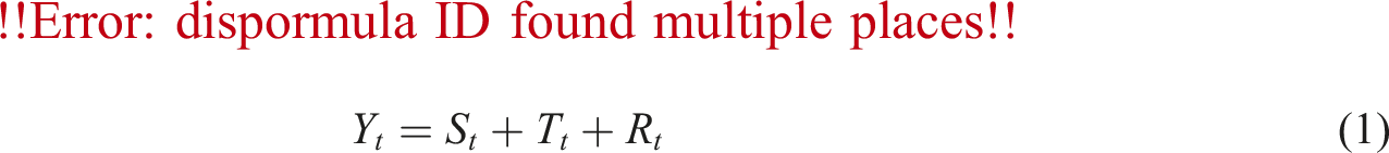
Developed by Cleveland et al., 1990, STL is a classical time series decomposition method that employs an algorithm based on locally weighted regression. This technique enhances data decomposition, especially for seasonality. Unlike other classical seasonal decomposition models such as X12 and SEATS, STL allows for flexible adjustment of the sizes of the seasonal and trend shift windows. It also improves the model’s robustness through outer loops, thereby enhancing outlier treatment. The STL method decomposes the time series Y
t
into three components: the seasonal part S
t
, the trend part T
t
and the residual part R
t
. The decomposition equation is as follows:
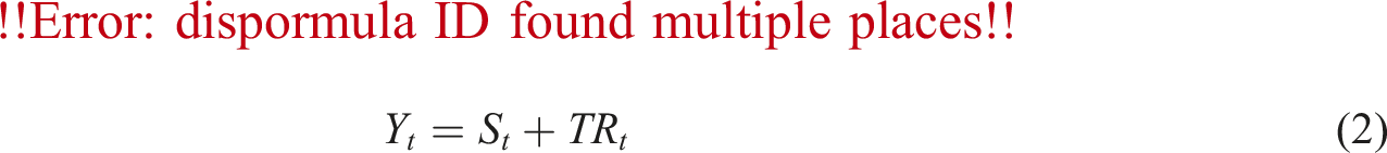
Abbreviating the trend part and the residual part, i.e. the part T
t
+ R
t
to TR
t
, and the expression becomes
Holt-Winters
The Holt-Winters seasonal model (Holt-Winters) is a widely used technique in time series analysis that utilizes the cubic exponential smoothing algorithm. Originally proposed by Winters in 1960, this model has been refined by researchers such as Cipra, Romera, and Hyndman. The Holt-Winters method is particularly effective for time series data that exhibit fixed periods, such as seasonal patterns. By decomposing the time series into its seasonal components, the method reduces seasonal noise and improves forecasting accuracy. This is especially useful when making multi-step-ahead forecasts for seasonal series. The updated equation for this model is:
Trend update:

Seasonal Updates:
Predicted value:
h-step-ahead forecasting values:
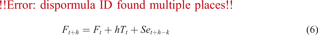
Where k is the period length, S t is the true value of the sequence, and α, β, γ ∈ (0, 1) are the individual smoothing parameters.
ARIMA and SARIMA
ARIMA is a classical time series model. It combines autoregressive and moving average processes and difference variables. It is a member of the autoregressive moving average (ARMA) model family. The ARMA model is commonly used as a benchmark tool for forecasting the demand for tourism services (Hu and Song, 2020; Li et al., 2017, 2020; Pan and Yang, 2017; Park et al., 2017; Jun et al., 2018; Zhang et al., 2020). The ARIMA(p, d, q) model is written as:
Where B is the lag operator, and φ is the autoregressive terms, and θ is the moving average terms, and a t is white noise series.
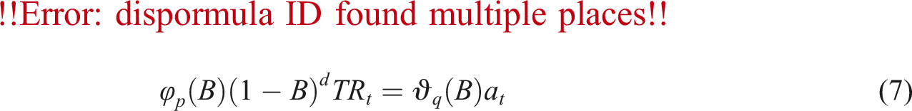
Seasonal ARIMA (SARIMA) can be used to account for the seasonality in tourist arrival data. The SARIMA model, an extension of the ARIMA model outlined by Box and Jenkins, is primarily a linear model applied to univariate time series. Over time, the SARIMA model has been developed to incorporate both seasonal and non-seasonal components. The model can be denoted as SARIMA (p, d, q) (P, D, Q) , written as:
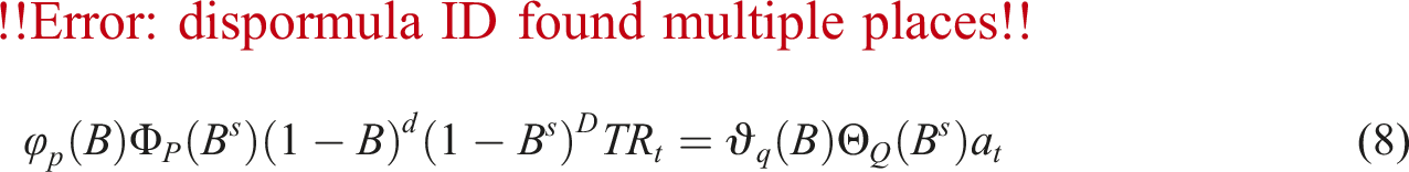
where p, q, and d represent the autoregressive (AR) term order, moving average (MA) term order, and difference term, respectively, while P, Q, D represent the seasonal AR term order, MA term order, and seasonal difference term order, respectively. Generally, P and Q range from 0 to 3, D ranges from 0 to 1, and s represents the length of the fixed period, the frequency of seasonal fluctuations in the time series. B is the lag operator and B s is the seasonal lag operator, and φ, Φ are the autoregressive and seasonal autoregressive terms, and ϑ, Θ are the moving average and seasonal moving average terms, and a t is white noise series. In this paper, we use the “auto.arima” function built in the “forecast” package of R statistical software to automatically select the optimal parameters for ARIMA/SARIMA models (Hyndman et al., 2020).
eXtreme gradient boosting (XGBoost)
XGBoost is a boosted tree algorithm proposed by Chen and Guestrin, 2016. This algorithm integrates multiple decision tree models using the gradient boosting method, ensuring interpretability while improving prediction accuracy. The boosted tree XGBoost employs additive operations to combine several base models, creating a strong learner. By incorporating dependencies among weak learners and utilizing sparse matrix storage for multi-threaded computation, XGBoost is significantly faster than other typical learners. It also effectively captures non-linear trends and reduces variance through the inclusion of a regular term, thereby preventing overfitting. The general expression for the model is:
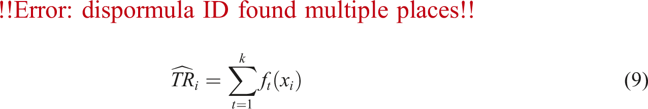
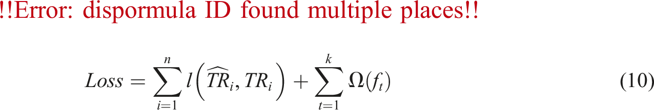
Here, k represents the number of base learners, and f denotes the base learner. The expression of the loss function with the inclusion of the regular term is given by:
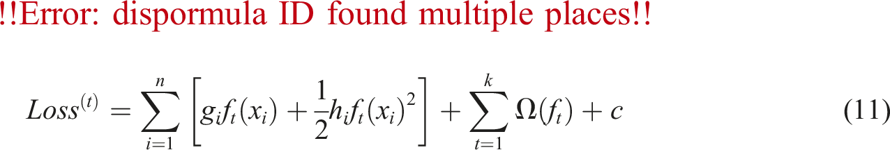
Where Ω represents the canonical term. The objective function is solved using Taylor expansions. By leveraging the property of summing basis functions and the fact that the predicted value of tree t − 1 is known when predicting tree t, we arrive at:
Here, g
i
is the first order derivative of
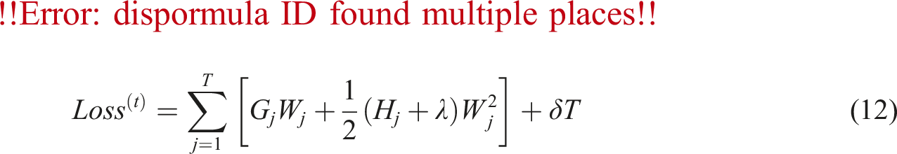
where G
j
=
Methodology
Proposed model
We construct a STL-XGBoost model, which combines the advantages of STL, Holt-Winters, ARIMA and XGBoost.
The Holt-Winters method is one of the most commonly used techniques in the Exponential Smoothing family of forecasting models. It is interpretable, requires fewer control parameters, and can be easily automated. Additionally, it adapts well to changes in trends and seasonal patterns in time series data as they occur. There are two variations of Holt-Winters, which differ in their treatment of seasonality: additive and multiplicative. These variants are more flexible in handling seasonality compared to the SARIMA model. As mentioned above, ARIMA is widely used in demand forecasting. It employs differencing to convert a non-stationary time series into a stationary one, and utilizes autocorrelations and moving averages of residual errors to forecast future values. It performs well on short term forecasts.
The specific flow chart is shown in Figure 1. The proposed model can be divided into five steps: 1) Input the original tourist arrivals time series. 2) STL decomposition is used to decompose the time series into two compenents: seasonal term and de-seasonal term (Trend + Residual terms). 3) For the seasonal term, model with Holt-Winters to obtain the forecasting result. 4) For the de-seasonal term, model with ARIMA first, then model with XGBoost model to obtain the forecasting the de-seasonal term. 5) The final forecasting tourist arrivals can be obtained by adding the Holt-Winters model’s forecasting result to the XGBoost model’s forecasting result. Flow chart for STL-XGBoost models.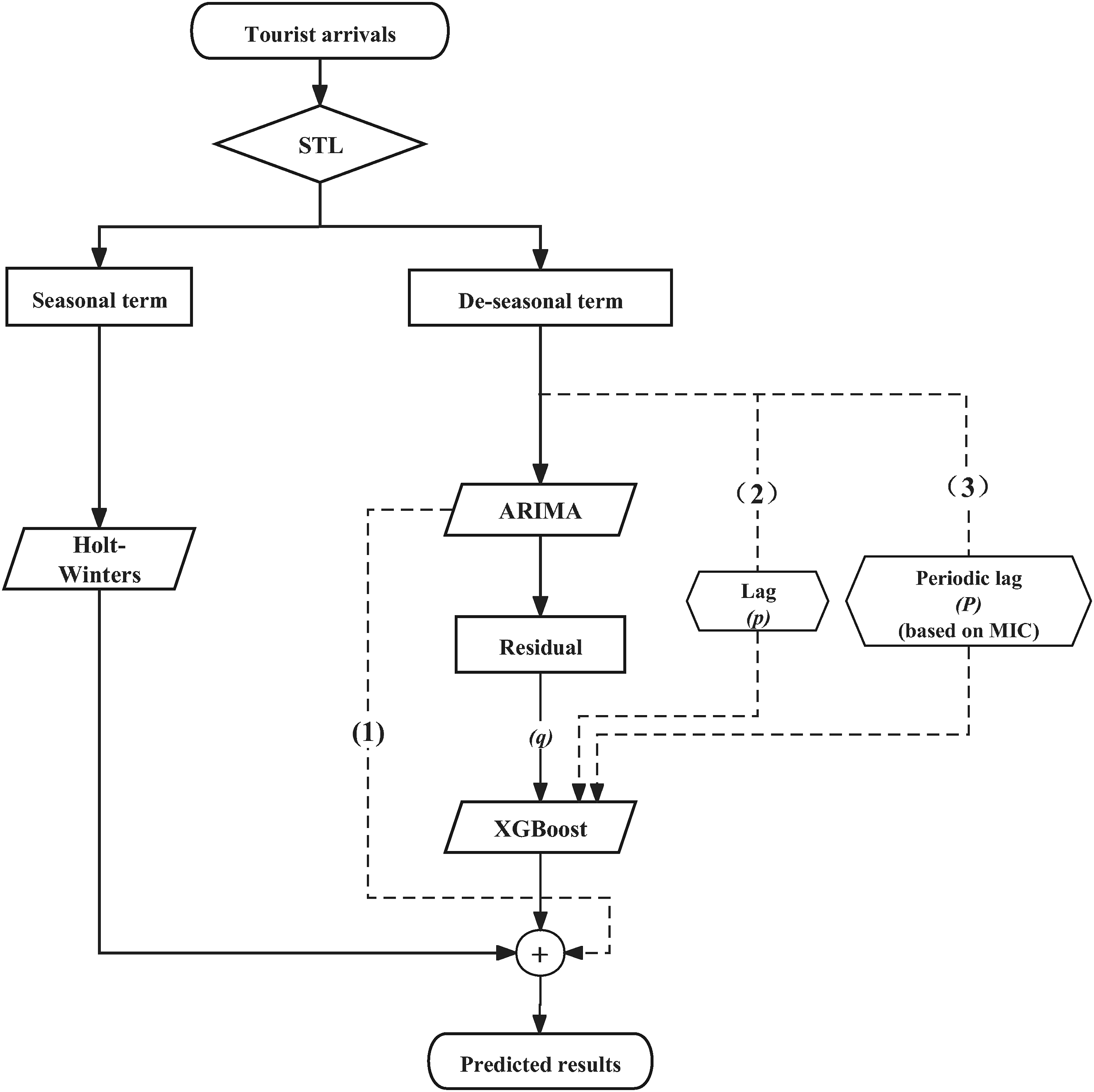
It is important to note that the fitting phase of Step 4 consists of two stages. During the first stage, the residual series (e t ) is generated from the de-seasonal term (TR t ) using an autoregressive integrated moving average (ARIMA) model. In the second stage, three different situations were considered to propose three different models.
The first model involves using the ARIMA residual series (e t ) as input for the XGBoost model to obtain the forecasting result. This model is denoted as SLT-XGBoost (1).
The second model incorporates both the ARIMA residual series (e t ) and the de-seasonal series (TR t ) as input for the XGBoost model to obtain the forecasting result. This model is denoted as STL-XGBoost (2).
The third model includes the ARIMA residual series (e t ), the de-seasonal series (TR t ), and the lagged periodic series as inputs for the XGBoost model to obtain the forecasting result. This model is denoted as STL-XGBoost (3). The decision to include the lagged periodic series in the STL-XGBoost (3) model is based on the calculation of the Mutual Information Coefficient (MIC) (Kinney and Atwal, 2014) for the series. MIC is an effective correlation measure that is capable of capturing a wide range of both functional and non-functional relationships between variable pairs in datasets. MIC can provide a more comprehensive measure of dependency not just linear or monotonic.
The key innovations of this method are as follows: 1) It utilizes STL seasonal decomposition to split the original time series without directly forecasting the seasonal series, effectively resolving bias issues arising from seasonal series forecasting in modeling tapes; 2) Different methods are employed to model the different components of the decomposition, leveraging the advantages of each model; 3) The inherent assumptions of the model, specifically the linearity and non-linearity of the components, are taken into account to enhance prediction accuracy; 4) Instead of employing complex network models for prediction, only interpretable models are used, enhancing interpretability while improving prediction accuracy.
Data collection
To evaluate the performance of our proposed model, we conducted empirical studies using Macau as our research subject. Macau is a world-renowned tourist destination and a Chinese special administrative region, attracting a constant influx of international tourists on a daily basis. Due to its reunification with China and subsequent rapid economic growth, tourism has become a major industry in Macau, contributing to over 40% of the total output in the 20th century. Therefore, analyzing short-term tourist arrivals in Macau is vital for both the Macau government and businesses to gain a comprehensive understanding of future market trends and changes (Song and Witt, 2006). This, in turn, leads to improvements in the quality and standards of tourism services.
For this study, we collected monthly tourist arrival data in Macau from eight countries: United States, Germany, Malaysia, Philippines, India, Thailand, Italy and Korea (South Korea). The data spanned from January 2009 to December 2018 and consisted of a total of 120 observations for each country. The data were sourced from the official website of the Macau Government Tourist Office (https://macaotourism.gov.mo). As shown in Figure 2, there is considerable volatility in the arrivals from these countries, with seasonal and cyclical patterns, as well as trends and random fluctuations, arising from nonlinear dynamics. Time series plots of tourist arrivals from eight countries.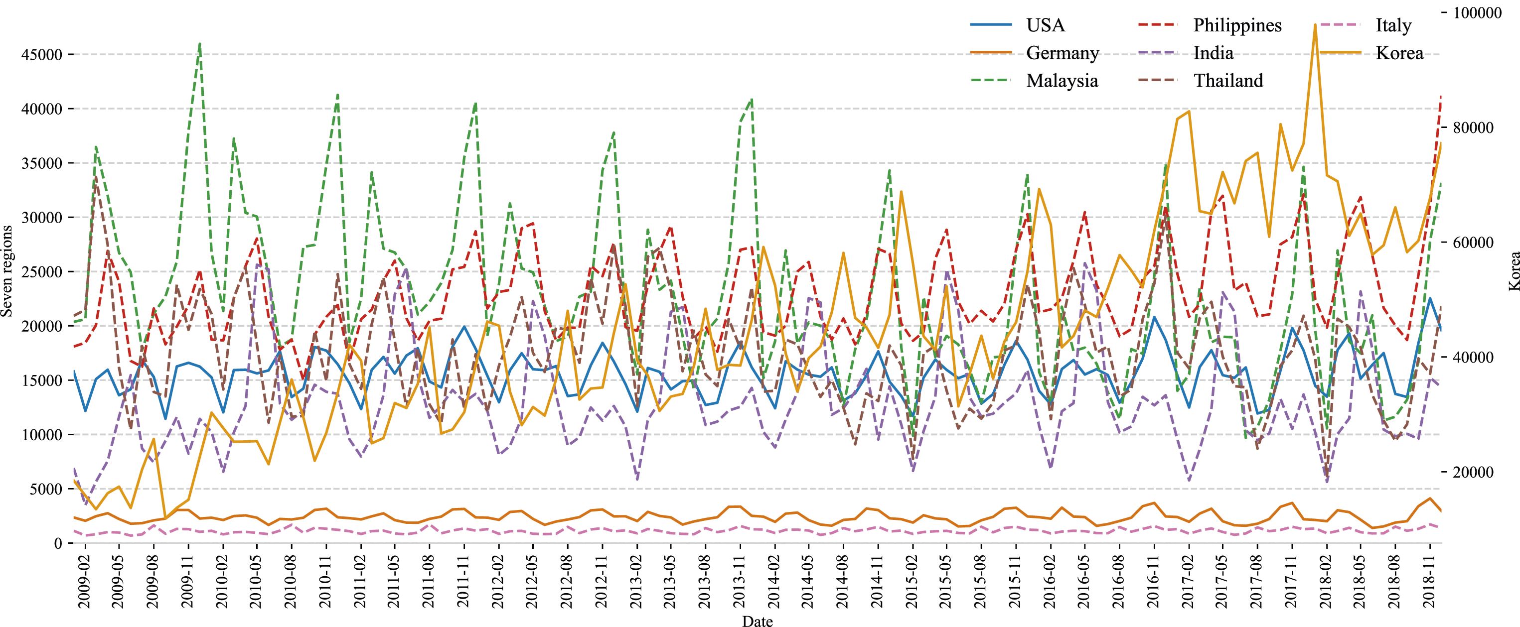
To train and evaluate our model, we split the original data set into a training set and a testing set at a ratio of 9:1. The training set consisted of data from January 2009 to December 2017, totaling 108 observations, while the test set encompassed data from January 2018 to December 2018, comprising 12 months of data. Addtionally, we employed a specific time series cross-validation method for selecting the optimal hyper-parameters of the proposed model (Hasan et al., 2020; H. Assaad and Fayek, 2021). As time series data are made up of neighboring data points that are often highly dependent on each other, standard cross-validation is not appropriate. The hyperparameters have been tuned prior to the training and testing of the model. In order to avoid introducing bias, a grid search time series cross-validation was performed on the training set to identify the optimal combination of hyperparameters. Grid search involves evaluating multiple combinations of hyper-parameters for the model. Due to the length of the time series being studied, a repeated 5-fold time series cross-validation was used. Using this cross-validation approach, the training set expands with each consecutive split selected in advance, while the test window size remains constant and shifts sequentially until the fifth and final split. There are two reasons why repeated time series cross-validation is momentous: firstly, it ensures robustness by accessing performance across different periods; secondly, it prevents information leakage from future data points by respecting chronological order. The selection of hyper-parameters was based on achieving high performance while ensuring generalization (i.e., avoiding overfitting). Thus, we quantified model performance by averaging prediction errors over these five splits. Based on the aforementioned, the data partitioning protocol employed in this study is as follows (as depicted in Figure 3): (1) employ time series split 5-fold cross-validation on the training set; (2) assess the model’s performance on each of the five validation splits for every iteration; (3) determine the hyper-parameters of the computational model based on minimizing averaged prediction errors; (4) evaluate the final performance of the proposed model on the unseen test set. 5-fold time series cross validation.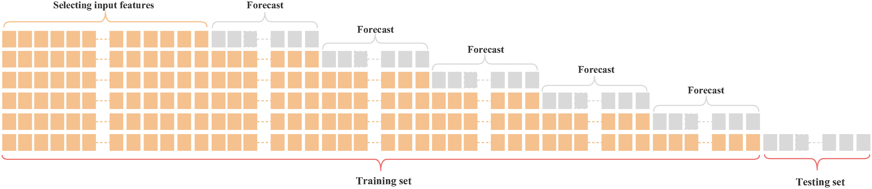
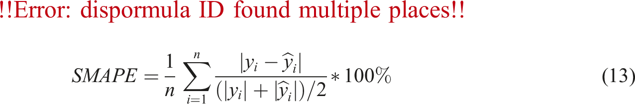
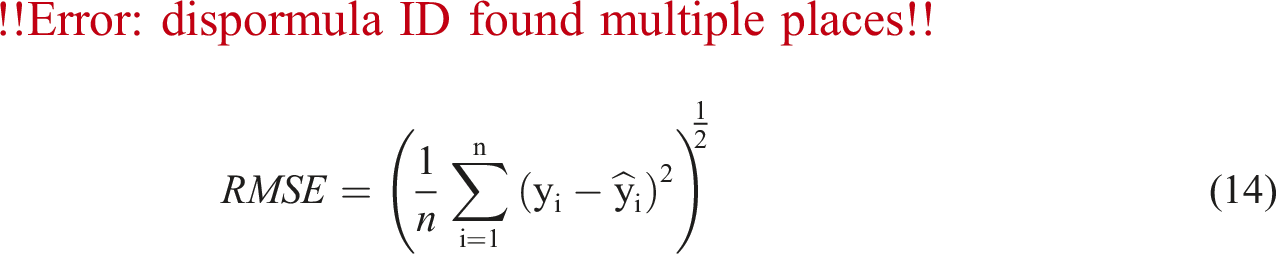
Evaluation indicators
To comprehensively evaluate the performance of the proposed models, we employ a set of evaluation indicators that offer different perspectives. These indicators include Symmetric Mean Absolute Percent Error (SMAPE), Root Mean Squared Error (RMSE), Mean Absolute Error (MAE), and Mean Absolute Percentage Error (MAPE). The mathematical formulas for these metrics can be found below.
where y
i
is the actual number of tourist arrivals and
Process and results
According to the workflow shown in Figure 1, the tourist arrivals data are firstly decomposed by STL decomposition. The decomposed components include seasonal term, trend term and residual term, and the last two terms are combined to form the de-seasonal term, as shown in Figure 4. In Figure 4, there are a total of five subgraphs from top to bottom. The first subgraph is the actual tourist arrivals graph (Y
t
) (taking Malaysia for example) and the second to fourth subgraphs are the seasonal (S
t
), trend (T
t
) and residual (R
t
) term that decomposed by STL decomposition. The fifth subgraph is the de-seasonal term (TR
t
= T
t
+ R
t
). STL seasonal decomposition results.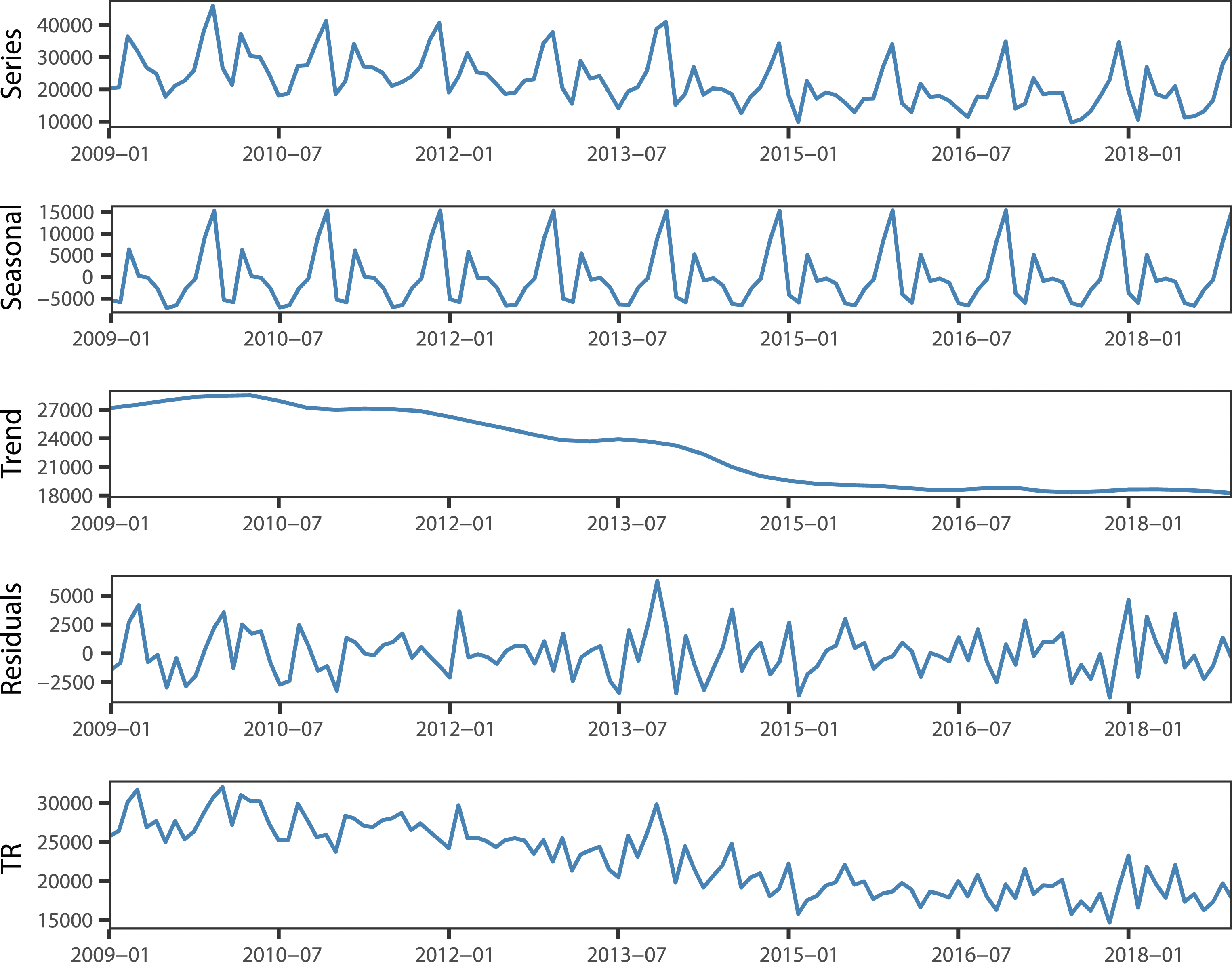
For the seasonal term (S t ), the Holt-Winters model is used to fit it to obtain the seasonal forecasting result. For the de-seasonal term (TR t ), the ARIMA model is firstly employed to fit it and generate the residual series (e t ). Then, three different situations were considered to put into the XGBoost model to obtain the de-seasonal forecasting result. XGBoost (1) model incorporates the ARIMA residual series as input to obtain the forecasting result; XGBoost (2) model incorporates both the ARIMA residual series (e t ) and the original de-seasonal series (TR t ) as input to obtain the forecasting result; STL-XGBoost (3) includes the ARIMA residual series (e t ), the original de-seasonal series (TR t ), and the lagged periodic series as inputs to obtain the forecasting result. Here the Mutual Information Coefficient (MIC) is employed to evaluate if there are periodical correlation between the de-seasonal series (TR t ). (See Appendix Table 1A for the results of MIC). The MIC values of the original de-seasonal series and the period lag are mostly larger than 0.25, which indicate significantly intra-periodical and periodical correlations. Finally, the tourist arrivals forecasting can be obtained by adding the Holt-Winters model’s forecasting result to the XGBoost model’s forecasting result.
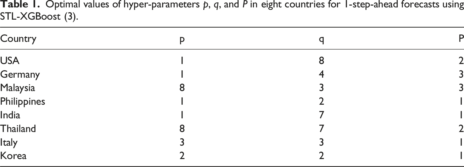
Optimal values of hyper-parameters p, q, and P in eight countries for 1-step-ahead forecasts using STL-XGBoost (3).
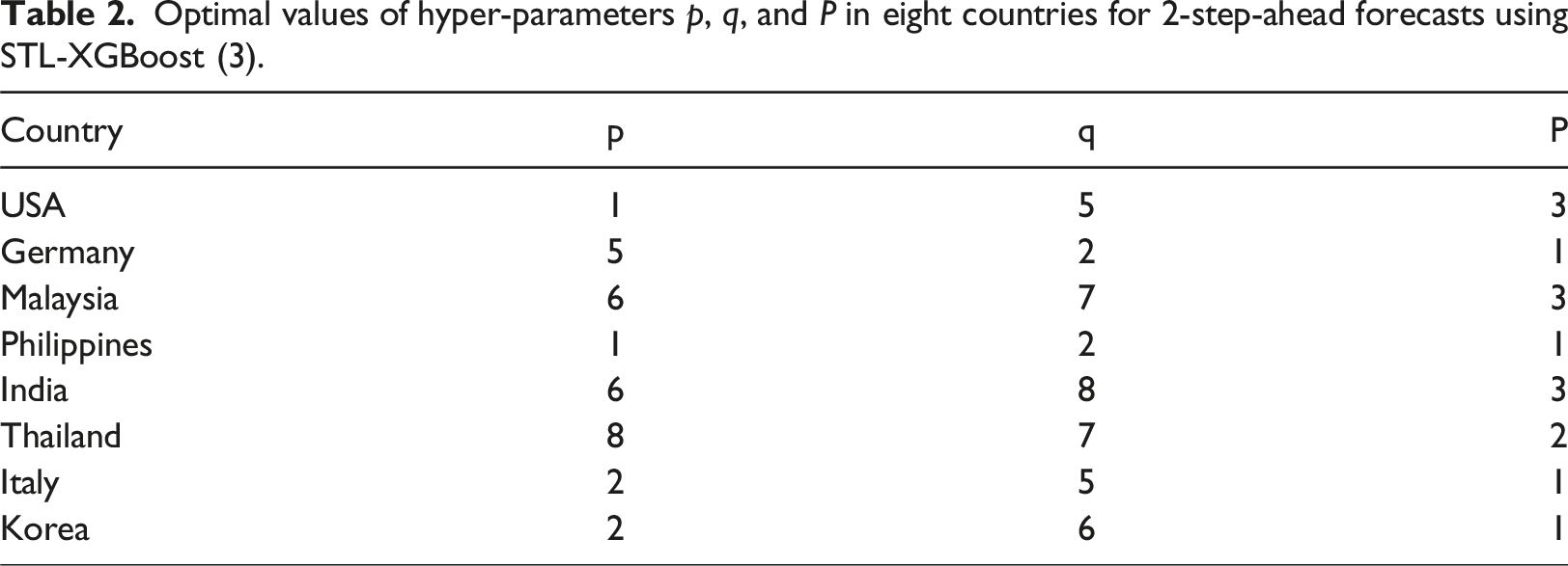
Optimal values of hyper-parameters p, q, and P in eight countries for 2-step-ahead forecasts using STL-XGBoost (3).
Optimal values of hyper-parameters p, q, and P in eight countries for 3-step-ahead forecasts using STL-XGBoost (3).

We constructed a comparative analysis of our proposed STL-XGBoost (1), STL-XGBoost (2), and STL-XGBoost (3). To test the forecasting performance of the proposed models, the h-step-ahead (h = 1,2,3) out-of-sample forecasts were generated. The out-of-sample prediction period was selected as 12 months. Based on the data from January 2009 to December 2017, a preliminary in-sample estimation of all models was performed. Subsequently, the estimates were computed continuously by including one observation at a time up to December 2018.
Prediction performance indicators such as SMAPE, RMSE, MAE and MAPE were calculated for each model as these metrics are commonly used in tourism demand forecasting. Using SMAPE as an example, relative comparisons have been made on the basis of the improvement of Model A over Model B, which has been calculated as follows:
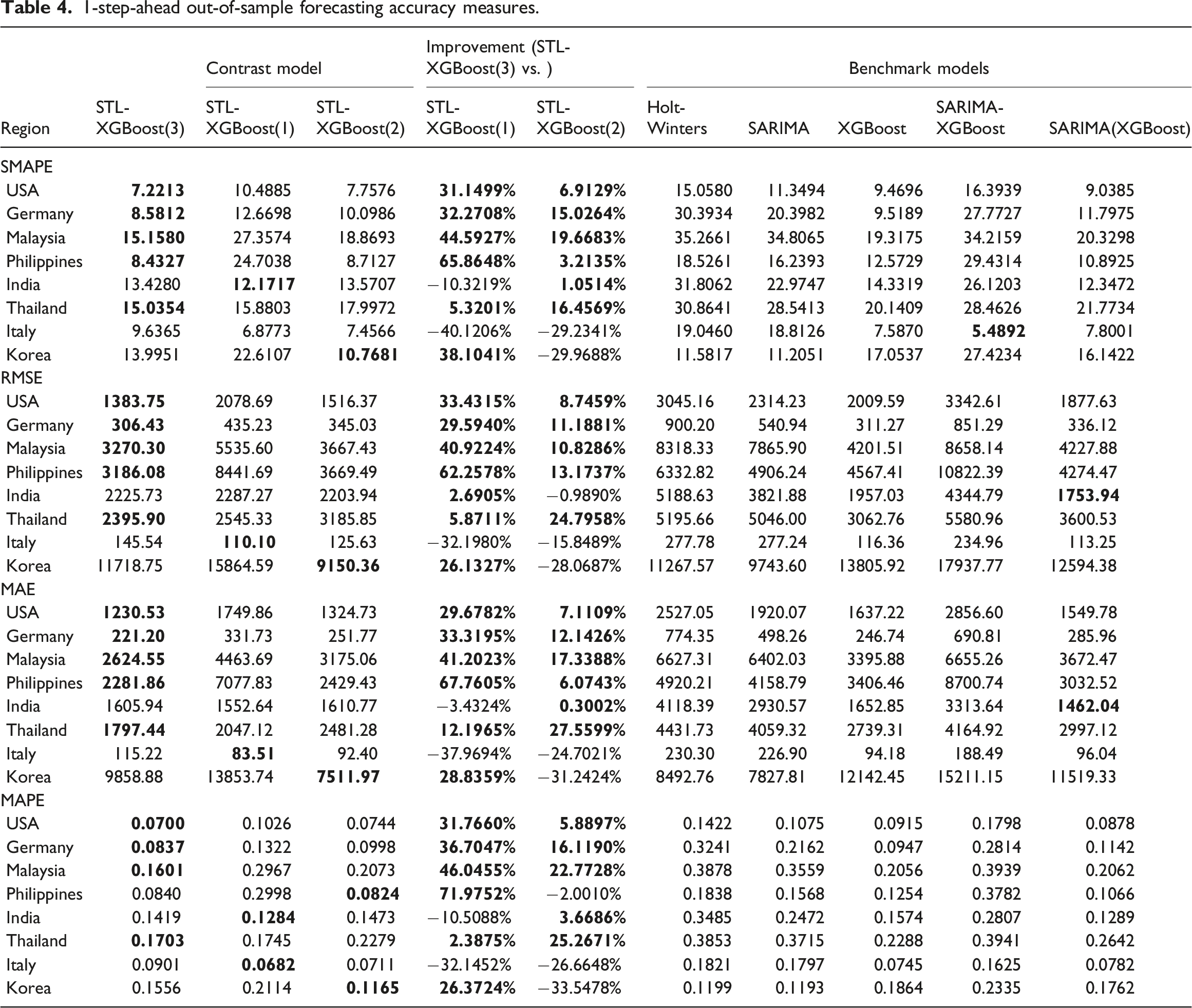
1-step-ahead out-of-sample forecasting accuracy measures.
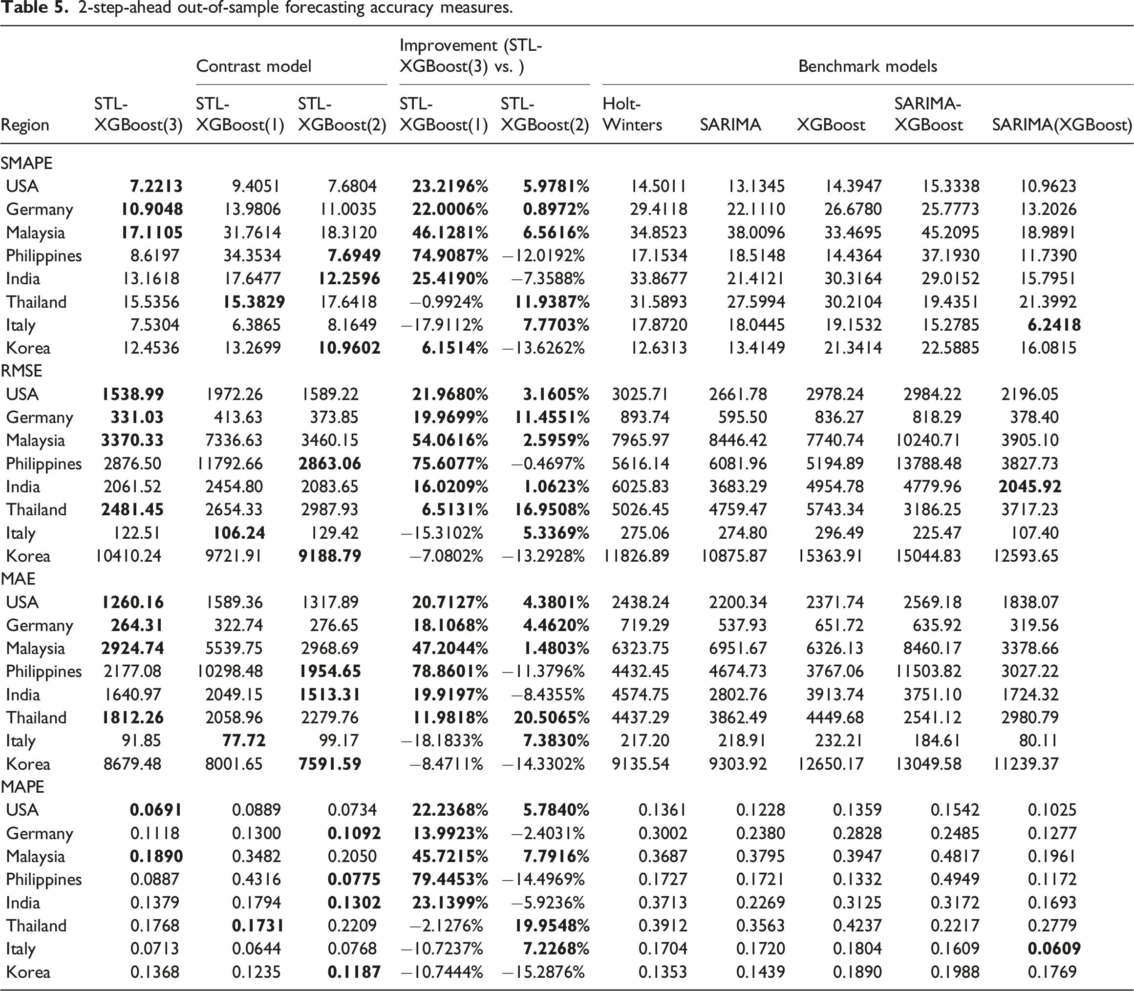
2-step-ahead out-of-sample forecasting accuracy measures.
3-step-ahead out-of-sample forecasting accuracy measures.
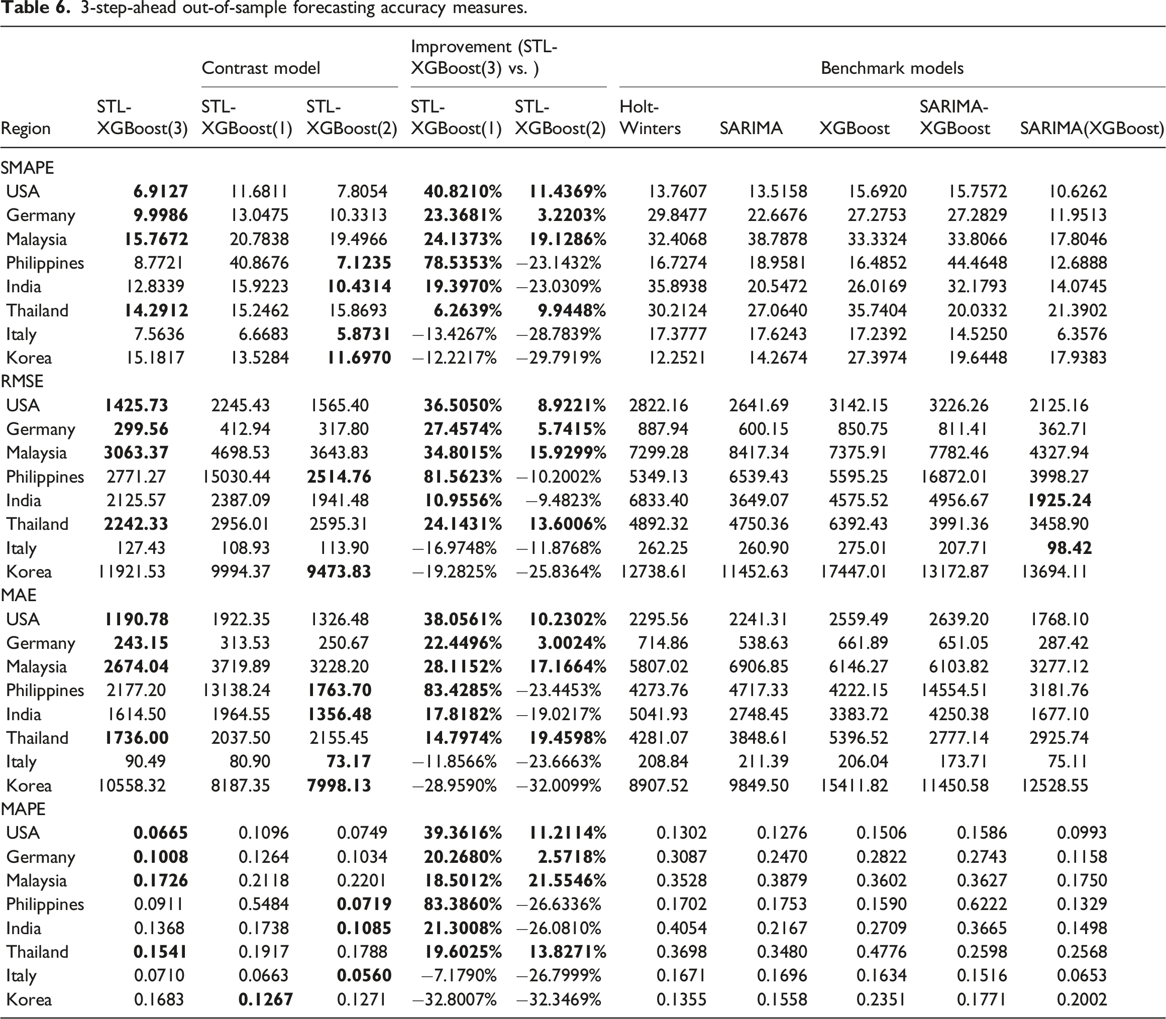
The results of the improvement in Tables 4–6 show that, compared with STL-XGBoost(1), the STL-XGBoost(2) and STL-XGBoost(3) model improved the forecasting accuracy for most source countries under consideration. Metrics such as SMAPE, RMSE, MAE, and MAPE also indicate better performances. Among them, the STL-XGBoost(3) model performs the best, followed by the STL-XGBoost(2) model. In terms of short-term forecasting accuracy for 1-step-ahead prediction, the STL-XGBoost(3) model outperforms others in most source markets. The improvements observed in this study mostly exceed 10%, indicating a significant enhancement in forecasting accuracy for short-term predictions. For long-term forecasting with 2- and 3-step-ahead predictions, both STL-XGBoost(2) and STL-XGBoost(3) exhibit even more remarkable improvements over STL-XGBoost(1).
It is noteworthy that the STL-XGBoost(2) model exhibits superior forecasting accuracy for predictions compared to the STL-XGBoost(3) model in the case of Korea. The time series plot depicting tourist arrivals from Korea reveals a consistent upward growth trend, with numbers escalating from 10,000 to nearly 80,000 (refer to Figure 2). This pattern distinguishes itself from other countries under consideration. A similar finding can be found in reference Song and Witt, 2006. Even in this scenario, our proposed STL-XGBoost(2) model demonstrates optimal performance primarily due to the robust trend observed in tourist arrivals from Korea. Consequently, when forecasting for Korea, greater emphasis should be placed on trend analysis as disturbances have negligible influence. Moreover, it is evident that the accuracy of 3-step-ahead forecasts by the STL-XGBoost(2) model surpasses that of STL-XGBoost(3) for Italy as well. Tourist arrivals from Italy have remained relatively stable without significant disruptive factors; henceforth only lag needs to be incorporated into residuals while periodic lag becomes unnecessary. Therefore, particularly for long-term predictions, the STL-XGBoost(2) model without periodic lag may outperform the STL-XGBoost(3) model with periodic lag.
These comparison findings verified the positive roles of including the ARIMA residual series, the de-seasonal series, or the lagged periodic series as inputs for the XGBoost model to obtain the predicted data. It helps to better fit the data and improve forecasting ability and performance.
On one hand, just includes the ARIMA residual series as input for the XGBoost model may hinder the prediction accuracy because the model only learns the residual’s nonlinearity. On the other hand, both empirical observations and the MIC values suggest a association between de-seasonal series and periodic lag series within specific short-term periods. Therefore, it is crucial to consider these series. In other words, the forecasting of the de-seasonal term is still affected by the periodical lag in short term prediction. Therefore it is essential to incorporate both the lag term and the periodic lag term together with the ARIMA residual term into the XGBoost forecasting model for accurate short-term predictions.
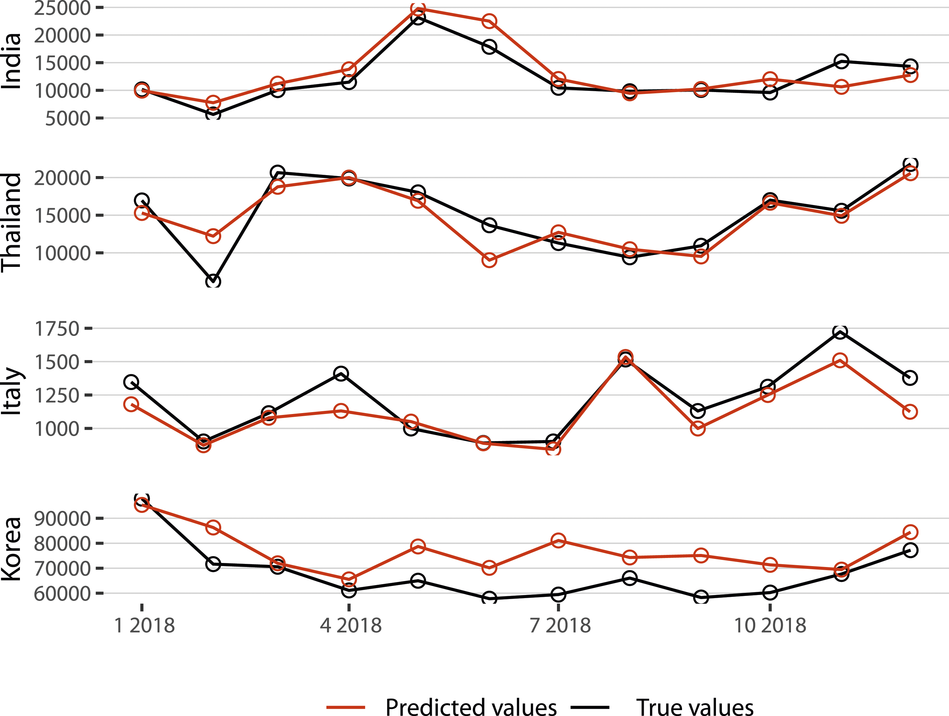
Figures 5 and 6 also display the predicted tourist arrivals from the countries under considered for the next 1 month based on STL-XGBoost(3) which is the one model of STL-XGBoost models. The results clearly indicate that the predicted arrivals are quite close to the actual tourist arrivals in Macau. The directional shifts in the actual and predicted values are consistent, demonstrating that the increases and decreases in the predicted values are consistent with the actual fluctuations in the tourist arrival time series. This holds true even for countries such as the United States, Philippines, and Thailand, which exhibit abrupt change points. Forecasts of tourist arrivals from the top four countries in Macau. Forecasts of tourist arrivals from the last four countries in Macau.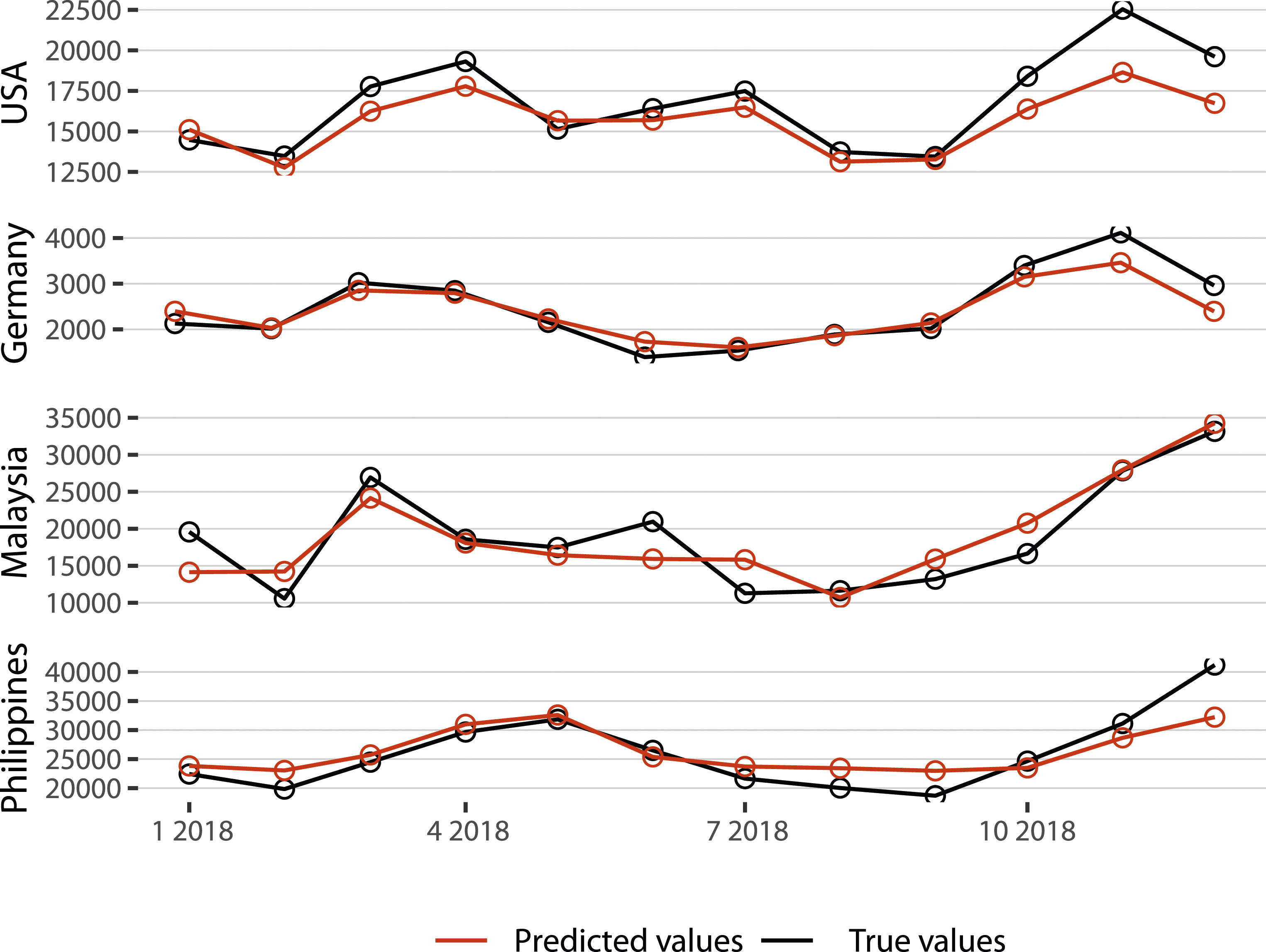
In order to show the forecasting performance of the proposed STL-XGBoost model more clearly, we present a comparative analysis of our proposed model, STL-XGBoost, with five other models. These include three benchmark models: SARIMA, Holt-Winters and XGBoost, as well as two hybrid models: SARIMA-XGBoost and SARIMA(XGBoost).
The SARIMA-XGBoost model was created by combining the SARIMA prediction and the XGBoost prediction, with the input being the SARIMA residuals. On the other hand, the SARIMA(XGBoost) model involved using the original tourist arrival data, its periodic lag and the SARIMA residuals as inputs for XGBoost prediction.
We also determined the optimal hyper-parameters for all the comparative models using the grid search method. Four evaluation indicators, namely SMAPE, RMSE, MAE, and MAPE, were employed to assess the forecasting performance. The prediction task involved estimating the tourists arrival from eight countries, including the United States, Germany, Malaysia, Philippines, India, Thailand, Italy and Korea in Macau. The models were evaluated for their ability to predict tourist arrivals 1 month, 2 months, and 3 months in advance. The comparison results are also presented in Tables 4–6.
The results of Tables 4–6 show that our proposed STL-XGBoost model, no matter it is STL-XGBoost(1), STL-XGBoost(2) or STL-XGBoost(3), has the most best forecasting performance of all the horizons of the forecast (h-step-ahead, i.e., h = 1,2,3) for all the countries under considered relative to five other models.
In particular, compared with SARIMA model, the reductions of STL-XGBoost(3) in SMAPE are 36.37%,57.93% 56.45%,48.07%,41.55%,47.32% and 48.78% in the case of 1-step-ahead forecasts for the seven countries under considered respectively, except for Korea. Compared with Holt-Winters and XGBoost, the reductions of STL-XGBoost models in SMAPE are quite significant. The reason behind the inferiority of SARIMA and Holt-Winters relative to STL-XGBoost model are that these two benchmark models are not capable of efficiently capturing nonlinear patterns and more sensitive to the outliers of tourism data. The worse performance of the XGBoost is due to that it is not capable to capture the seasonal components of tourism data.
The SARIMA-XGBoost hybrid model was used for predicting seasonal characteristics. However, its ability to reduce prediction errors compared to benchmark models is not consistently apparent. The results show mixed outcomes, with improvements in some cases and decreases in others, indicating that the model lacks stability. Therefore, using simple a additive of linear and nonlinear models for prediction is not consistent better in most cases.
To address the impact of seasonal factors on the nonlinear model and avoid assuming a simple linear and nonlinear additive relationship, the SARIMA model prioritized deriving residuals. In addition to incorporating the model-derived residuals, original sequence and the periodic lag part were included in the XGBoost model. This allowed the model to learn multiple nonlinear relationships, resulting in the SARIMA(XGBoost) model. The prediction results show that the SARIMA(XGBoost) model generally performs better than benchmark models that rely solely on linear or nonlinear models, or a combination of both. However, when compared to our proposed STL-XGBoost models, the SARIMA(XGBoost) model performances worse in terms of prediction accuracy and precision. The reduction of STL-XGBoost models except for India, in SMAPE is about 10%-30% compared with SARIMA(XGBoost).
Therefore, based on the comparison with the SARIMA-XGBoost and SARIMA(XGBoost) hybrid models, it is beneficial to extract and model the seasonal term separately. This approach results in overall smaller errors and improves prediction performance.
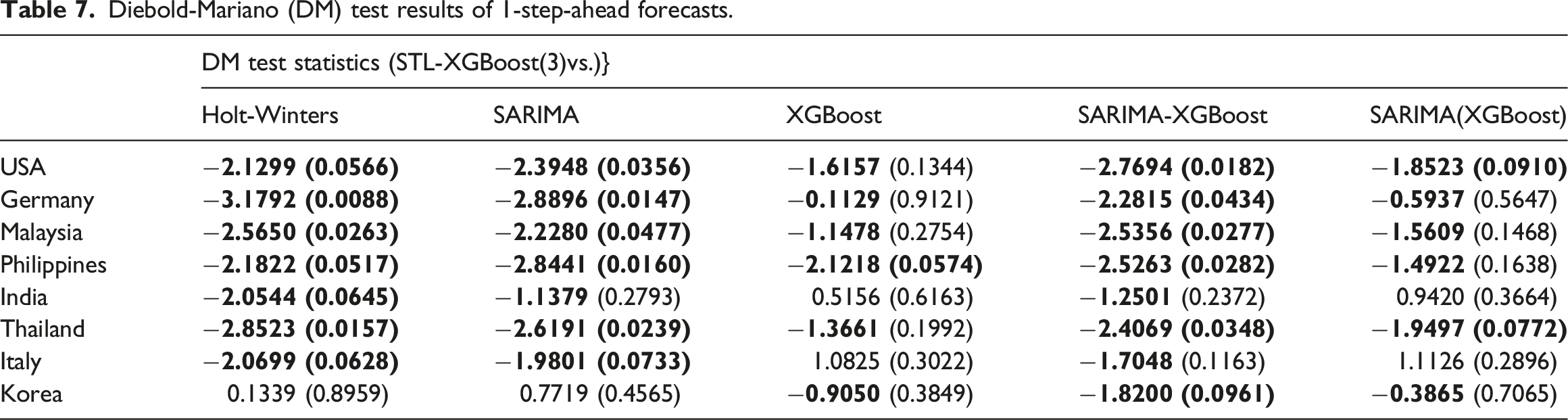
Diebold-Mariano (DM) test results of 1-step-ahead forecasts.
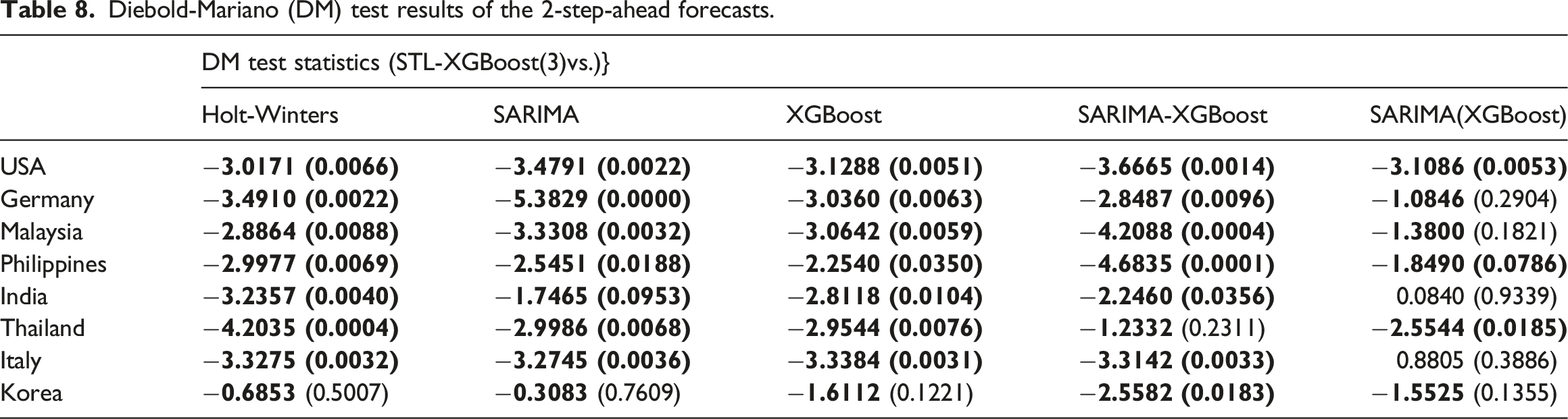
Diebold-Mariano (DM) test results of the 2-step-ahead forecasts.
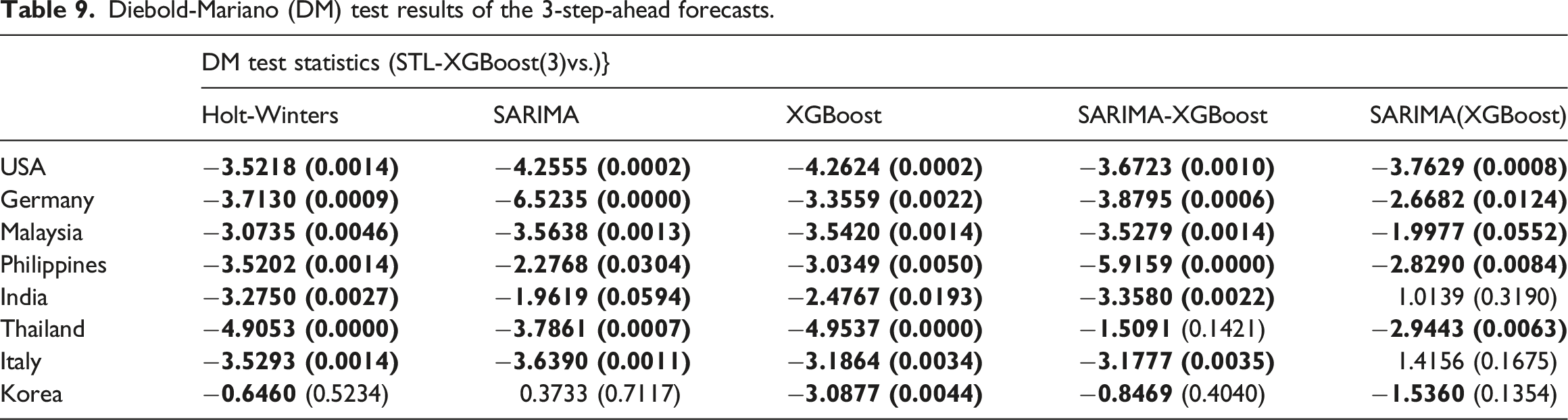
Diebold-Mariano (DM) test results of the 3-step-ahead forecasts.
Discussion and conclusions
In this study, we proposed a forecasting model called STL-XGBoost to address the challenge of predicting tourist arrivals with seasonal and trend characteristics. The model effectively overcomes the limitations associated with non-stationary, non-linear, and seasonally complex time series models.
To achieve this, we employed STL seasonal decomposition to decompose the time series data into two components: the seasonal term and the de-seasonal term. By individually modeling these terms, we were able to effectively analyze and capture the seasonal patterns, trends and noise in the tourist arrivals data.
For the seasonal components, we utilized the Holt-Winters model, which has been widely used for modeling time series data with seasonal patterns. This allowed us to accurately capture the seasonal effects on tourist arrivals. For the de-seasonal components, we employed the ensemble learning model XGBoost. Unlike traditional non-linear models, XGBoost offers greater interpretability, speed, and stability. By considering both the lagging factors and the causal effects induced by these factors, our model mitigates the assumptions of a simplistic linear additive relationship as observed in the ARIMA model in the de-seasonal components.
Furthermore, our STL-XGBoost model exhibits scalability, generalizability, and wide applicability. It comprehensively considers the seasonal characteristics, the coexistence of trend stochastic and non-linear features, and effectively handles the complexity and uncertainty of tourist arrivals data. It provides a more accurate and reliable forecasting tool for predicting tourist arrivals with seasonal and trend characteristics.
Although our proposed STL-XGBoost model has demonstrated satisfactory predictive performance to some extent, we solely relied on time series data for prediction and did not consider other factors such as numerical features of holiday effects and economic fluctuations, as well as textual features of real-time policies that exert significant influence on tourist arrivals. Moreover, the uncertainty surrounding various factors often exceeds researchers’ initial assumptions. Additionally, empirical evidence reveals that the complexity of the tourism market cannot be fully addressed by a limited number of classical models. Therefore, it is anticipated that future research on modeling should integrate a wide range of factors, including text-based variables and interaction effects, while employing more adaptable techniques to develop highly accurate predictive models capable of effectively addressing the intricacies and uncertainties inherent in real-world tourism market.
Supplemental Material
Supplemental Material - Forecasting tourist arrivals using STL-XGBoost method
Supplemental Material for Forecasting tourist arrivals using STL-XGBoost method by Minmin He and Xiyuan Qian in Tourism Economics
Footnotes
Declaration of conflicting interests
The author(s) declared no potential conflicts of interest with respect to the research, authorship, and/or publication of this article.
Funding
The author(s) received no financial support for the research, authorship, and/or publication of this article.
Correction (May 2025):
In the published version of the article, there was an error in the article type listed in the header on the title page. It was previously listed as a “Review Article” but has now been corrected to “Research Article.” The article has been updated online to reflect this change.
Supplemental Material
Supplemental material for this article is available online.
Author biographies
References
Supplementary Material
Please find the following supplemental material available below.
For Open Access articles published under a Creative Commons License, all supplemental material carries the same license as the article it is associated with.
For non-Open Access articles published, all supplemental material carries a non-exclusive license, and permission requests for re-use of supplemental material or any part of supplemental material shall be sent directly to the copyright owner as specified in the copyright notice associated with the article.