A three-dimensional method for the simulation of temperature fields induced by solar radiation

Abstract

The determination of temperature fields is usually required for the calculation of structural deformation and stress induced by temperature variation. To guarantee the serviceability and safety of structures by improving calculation accuracy, this study presents a three-dimensional structural temperature field simulation framework that accounts for shadowing effects and changes in solar radiation intensity throughout the day. Field experiments were conducted to update the established model and to verify the accuracy of the numerical algorithm. The proposed method was finally applied in a case study to determine the temperature fields of both a rail and a U-shaped concrete girder. The results show that the temperature field of the concrete girder had obvious nonlinear distribution characteristics. Three-dimensional structural temperature field analysis is especially required for complicated structures with varied sections along the longitudinal axis.

Keywords

field experiments numerical calculation shadowing effects solar radiation temperature difference temperature field

Introduction

The deformation and stress caused by temperature variation are important factors that must be considered in the design and construction of structures such as machines, airplanes, buildings, and bridges. A structure’s temperature field can be generally divided into the uniform temperature and the gradient temperature. The uniform temperature causes expansion or contraction movement along the member’s axial length, whereas the gradient temperature induces bending deflections. Thermal stress can be then produced by these deformations in the structure. Thermal deformation and stress both have adverse effects on a structure’s serviceability and safety. Therefore, accurate determination of a structure’s temperature distribution has many applications in the design of prestressed concrete bridge girders (Barr et al., 2005), the assessment and selection of bridge expansion joints (Arockiasamy et al., 2008), the study of bridge performance using fiberglass-reinforced plastic and other new composite materials (Kong et al., 2014; Yu et al., 2008), the analysis of the thermal behavior of cracked concrete members in fire (Ervine et al., 2012; Wu et al., 2014), structural health monitoring of large bridges (Xia et al., 2013; Xu et al., 2010), and the study of track-bridge interactions in railway bridges (Mirza et al., 2015; Ryjáček and Vokáč, 2014) due to daily variations in temperature.

It was generally assumed in early studies that the temperature field within a beam component of a complex structure either remained steady or varied linearly along the beam height. Zuk (1965) derived an approximate formula for calculation of the maximum vertical temperature difference in the cross section of a concrete beam, with the assumption that the temperature distribution varies linearly over the beam height. Some scholars later realized the irrationality of the linear distribution assumption. For example, Priestley (1978) adopted a 5th power function to represent the internal temperature field of the concrete bridge, based on the theoretical model and on engineering practice. Churchward and Sokal (1981) suggested that it is more reasonable to use the hyperbolic function to express the nonlinear temperature distribution within the structure based on the measured data.

Because the geometry and boundary conditions of the temperature fields of real structures are usually very complicated, it is difficult to obtain an accurate temperature field by analytical methods. Numerical simulation has therefore become the most powerful method with which to estimate a structure’s temperature field. Earlier researchers such as Emerson (1973), Hunt et al. (1975), and Mirambell and Aguado (1990) used the finite difference method to solve the differential equation of heat conduction. Since then, the finite element method (FEM) has been more extensively applied to investigate the structural temperature field. Elbadry and Ghali (1983) developed a dedicated finite element program named FETAB to analyze the structural temperature field and used it to obtain the temperature distribution law of the two-dimensional (2D) section of both simply supported and continuous concrete box girder bridges. Branco and Mendes (1993) dealt with the temperature boundary condition with the use of Fourier transformation and proposed an FEM for calculation of the temperature field. Currently, the FEMs coded in commercial software ANSYS (Kong et al., 2014; Xia et al., 2013), ABAQUS (Lee, 2012; Mirza et al., 2015; Wu et al., 2014), and other general finite element software are widely used to establish the effects of temperature on a structure via finite element models. Although three-dimensional (3D) modeling of the temperature field is available with the use of an FEM, some researchers (Lee, 2012; Wen-shuo et al., 2014) have used a 2D model with the assumption that the temperature has a uniform distribution along the direction of the longitudinal axis. The advantage of such simplification is that the computation cost is greatly reduced; however, major errors may occur in the case of variable cross section or spatial shadow. Studies have shown that the temperature field calculated by the simplified method is not reliable (Hoffman et al., 1983), especially for complex structures such as concrete arch dams (Fleischer et al., 2004).

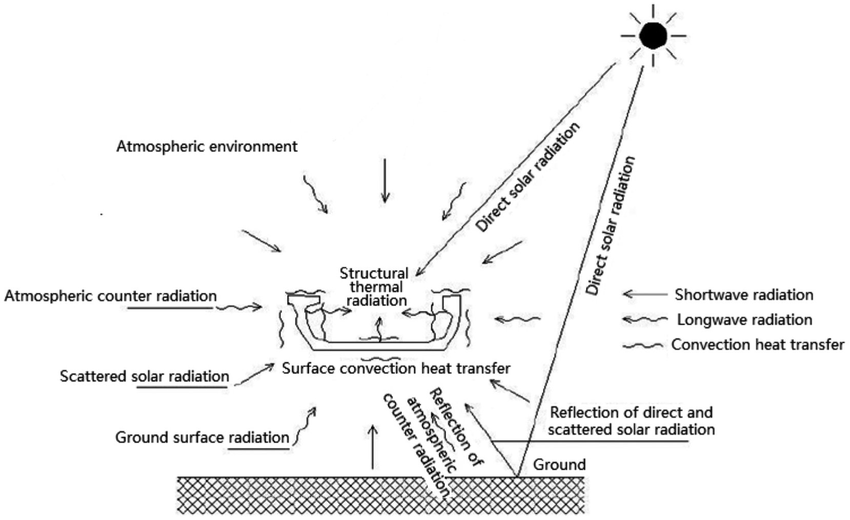
The difficulty of calculating the 3D structural temperature field lies mainly in determining a method to simulate thermal boundary conditions that change with time and space. In addition, due to the shadow produced by both the structure itself and the surrounding environment, not all of the parts of the structure are exposed to direct solar radiation, which is another important factor in the structural temperature field under sunshine. Numerous studies failed to account for the shadowing effect (Arockiasamy et al., 2008; Kong et al., 2014), which introduced errors to the calculation of the temperature field. Some studies deduced formulas to calculate the shadow covering in the plane for beam sections of specific structures such as box beams (Elbadry and Ghali, 1983) and I-shaped beams (Lee, 2012). However, it cannot be widely applied in general use, and the plane simplification also leads to certain errors.

In this study, a self-compiled program was used in combination with the general finite element software ANSYS to deal with the 3D temperature boundary conditions. The solar radiation intensity was determined based on the clear-sky model of the American Society of Heating, Refrigerating, and Air Conditioning Engineers (ASHRAE), and the model’s parameters were updated via solar radiation intensity tests. At the same time, the temperature field of the U-shaped concrete girder was tested to verify the accuracy of the numerical algorithm. A case study was conducted to calculate the temperature fields of both the railroad rail and the girder. Finally, investigations were conducted on the daily temperature distribution law of the girder and the relative temperature difference between the rail and the girder.

Numerical calculation method

Differential equations of heat conduction and temperature boundary conditions

Let T(x, y, t) denote the temperature of an object at the given position (x, y, z) and at time t. According to the principle of heat balance, the well-known heat conduction differential equation can be expressed as (Elbadry and Ghali, 1983)

\frac{\partial T}{\partial t} - \frac{λ}{c ρ} \nabla^{2} T = \frac{W}{c ρ}

(1)

where $ρ$ is the density of the object, c is the specific heat capacity, $λ$ is the thermal conductivity coefficient, and W is the intensity of the internal heat source. The solution of equation (1) requires the initial condition and the boundary condition. The initial condition can be written as

{(T)}_{t = 0} = f (x, y, z)

(2)

where f(x, y, z) is a known function that indicates the object’s temperature distribution at the moment t = 0.

Generally, the boundary condition can be given in three alternate ways by giving (1) the temperature of any point on the object’s surface at all instants, (2) the normal heat flux density of any point on the object’s surface, and (3) the condition of convection and heat release of any point on the object’s boundary at all instants. These three kinds of thermal boundary conditions can be expressed in a unified form

- λ \frac{\partial T}{\partial n} = - q + γ (T - T_{f})

(3)

where $\partial T / \partial n$ represents the directional derivative of the temperature along the normal direction of the boundary, q is the heat flow rate, $γ$ is the heat exchange coefficient, and $T_{f}$ is the ambient temperature. In this study, the third kind of thermal boundary condition is used in numerical calculation because the effects of solar radiation and atmospheric convection (see Figure 1) can be regarded as convective heat exchange in the numerical calculation.

Figure 1.

Boundary conditions for the simulation of temperature field.

Among these parameters, the determination of the heat exchange coefficient is one of the most important concerns in the calculation of structural temperature field. Some scholars (Moorty and Roeder, 1992; Prakash, 1986) have confirmed that the heat exchange coefficient is primarily controlled by the wind speed. An empirical formula provided by Prakash (1986) is adopted in this study (see Table 1) to determine the heat exchange coefficient.

Table 1.

Main parameters used in case study.

Parameters		Unit	Values
Location of girder	Location	–	Qingdao, China, 36N/120E
Location of girder	Girder azimuth angle	–	50° west of north
Material property of concrete	Density	$kg / m^{3}$	2650
	Thermal conductivity	$ω / (m k)$	2
	Heat capacity	$J / (kg k)$	930
	Total heat exchange coefficient	$ω / (m^{2} k)$	13.5 + 3.88v^a
	Longwave radiation absorptivity coefficient	–	0.88
	Shortwave radiation absorptivity coefficient	–	0.65
	Emissivity coefficient	–	0.88
Material property of rail	Density	$kg / m^{3}$	7830
	Thermal conductivity	$ω / (m k)$	80
	Heat capacity	$J / (kg k)$	465
	Total heat exchange coefficient	$ω / (m^{2} k)$	13.5 + 3.88v^a
	Longwave radiation absorptivity coefficient	–	0.55
	Shortwave radiation absorptivity coefficient	–	0.55
	Emissivity coefficient	–	0.8
Environmental parameters	Solar radiation intensity	$ω / m^{2}$	According to the ASHRAE clear-skytheory model based on experimentalcorrection
	Atmospheric cleanliness	–	0.8
	Structural initial temperature	°C	20
	Atmospheric temperature	°C	According to data from meteorological administration
	Wind speed	$m / s$	According to data from meteorologicaladministration

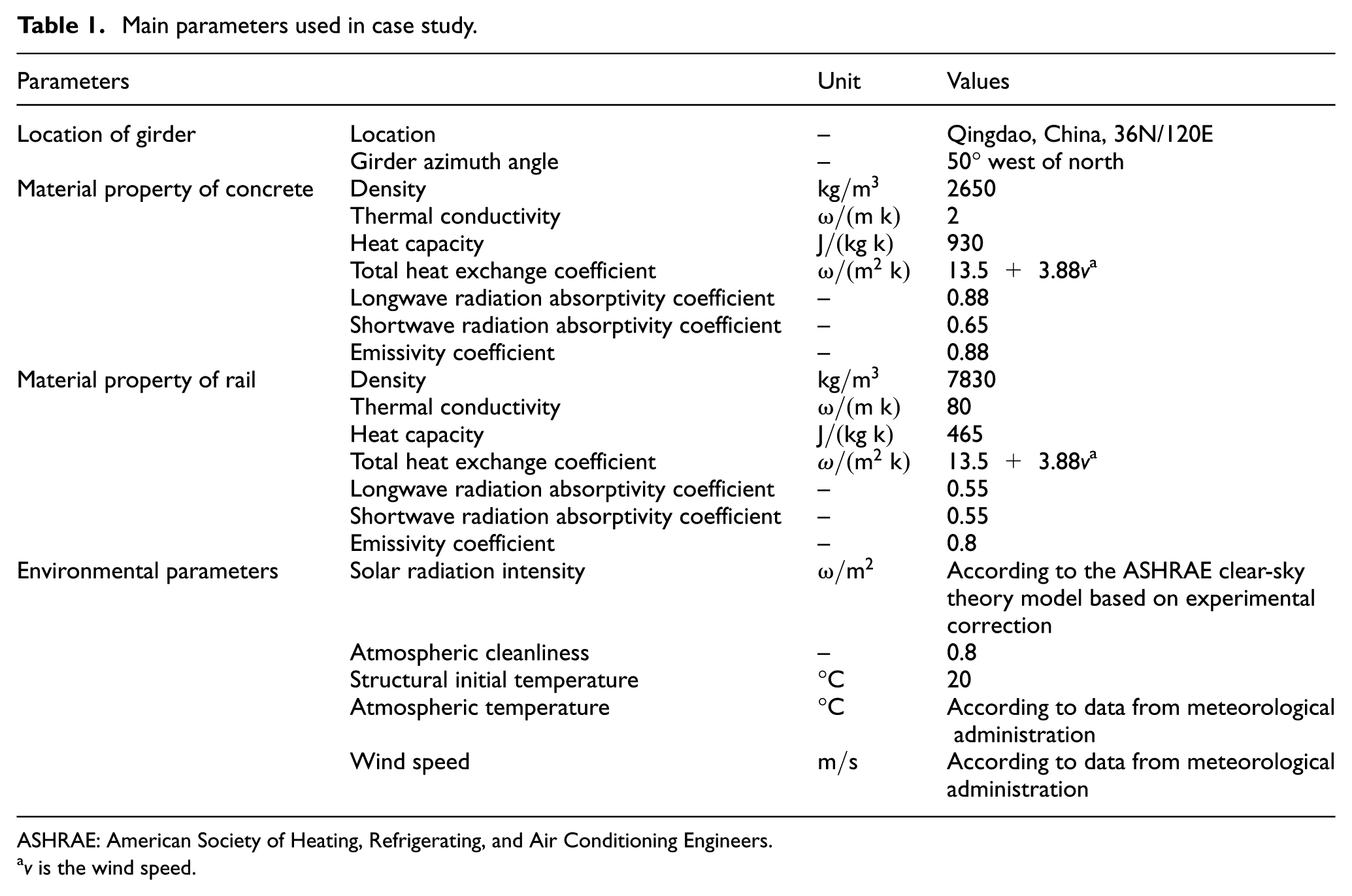
ASHRAE: American Society of Heating, Refrigerating, and Air Conditioning Engineers.

v is the wind speed.

Calculation of solar radiation directions

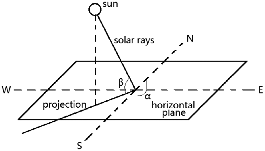
Solar radiation intensity is one of the most important factors in a structure’s temperature distribution (Elbadry and Ghali, 1983; Kehlbeck, 1981). It is determined by the solar altitude angle $β$ , the azimuth angle $α$ , and the structural incidence angle $θ$ (see Figures 2 and 3).

Figure 2.

Illustration of the solar altitude angle and the azimuth angle.

Figure 3.

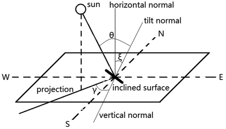
Illustration of the structural incidence angle.

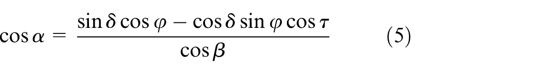
The solar altitude angle $β$ can be obtained as follows (Elbadry and Ghali, 1983; Kehlbeck, 1981)

\sin β = \cos φ \cos τ \cos δ + \sin φ \sin δ

(4)

where $δ$ is the solar declination angle, which is usually set to be 23°26′, $φ$ is the latitude angle of the location, and $τ$ is the solar hour angle, which is defined as the angle between two planes: one is the meridian plane containing the connecting line between the sun and the earth, and the other is the meridian plane containing the located position. The solar hour angle can be calculated according to the local time. The solar azimuth angle $α$ can be obtained as follows (Elbadry and Ghali, 1983; Kehlbeck, 1981)

\cos α = \frac{\sin δ \cos φ - \cos δ \sin φ \cos τ}{\cos β}

(5)

After obtaining the position of the sun in the sky determined by the solar altitude angle $β$ and the azimuth angle $α$ , the incidence angle $θ$ between the solar ray and the normal direction of the incident surface on the object can be expressed as

\cos θ = \cos β \cos γ \sin ξ + \sin β \cos ξ

(6)

where $ξ$ is the angle between the normal of the incident surface and the normal of the horizontal plane, and $γ$ is the angle between the projection of the solar rays and the vertical normal.

ASHRAE clear-sky model for the solar radiation intensity

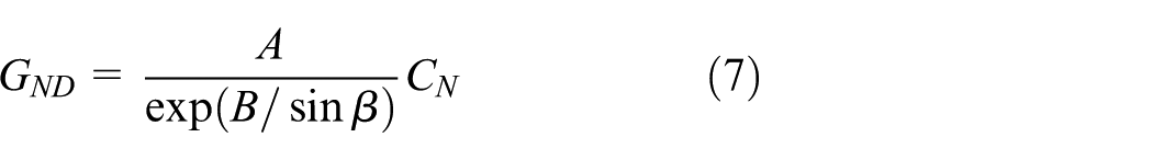
The clear-sky model recommended by ASHRAE has been widely used to calculate solar radiation intensity. According to the ASHRAE clear-sky model, the solar radiation received by a structure consists of three parts: direct solar radiation, diffuse solar radiation, and reflected solar radiation. The direct radiation intensity can be calculated with the following form (ASHRAE, 2001)

G_{ND} = \frac{A}{\exp (B / \sin β)} C_{N}

(7)

where $G_{ND}$ is the direct solar radiation intensity under the vertical incidence condition, A is the solar radiation intensity when the atmospheric mass is zero, B is the atmospheric extinction coefficient, $β$ is the solar altitude angle, and $C_{N}$ is the atmospheric cleanliness. The total absorbed solar radiation intensity to the nonvertical surface is the sum of the direct radiation, the sky scattering radiation, and the reflected radiation (ASHRAE, 2001)

G_{t} = ξ [\max (\cos θ, 0) + C \frac{(1 + \cos α)}{2} + ρ_{g} \frac{(1 - \cos α)}{2} (\sin β + C)] G_{ND}

(8)

where $G_{t}$ is the total radiation intensity of the structural surface, $ξ$ is the absorption rate of the solar radiation by the structural surface, C is the ratio of the diffuse radiation on a horizontal surface to the direct radiation with vertical incidence, $ρ_{g}$ is the ambient reflectance, $α$ is the inclination of the structural surface to the horizontal plane, and $θ$ is the incidence angle defined in equation (6).

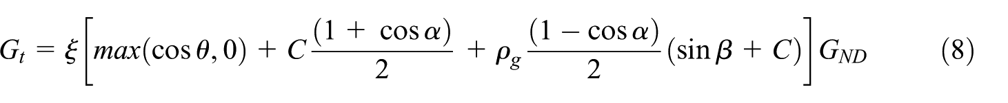
The main undetermined parameters in the ASHRAE clear-sky model are A, B, C, and $C_{N}$ , which were presented by (McQuiston, 1989) from regression fitting of the measured data of the solar radiation intensity in the United States. However, it is better to update these parameters from experimental data at specific locations. This issue is discussed in detail in section “Updating of parameters in ASHRAE model.”

Procedure of numerical calculation

To calculate the structure temperature field under sunshine, a 3D transient finite element model was established with ANSYS 16.0. Figure 4 shows an example of the finite element mesh for a U-shaped girder used in urban rail transit bridges. The hexahedral heat conduction element SOLID70 with eight nodes is used to model the structure temperature field. The surface element SURF152 on the structure’s surface is applied to receive the thermal convection and thermal radiation loads. The boundary condition of solar radiation is applied directly to the structure’s outer surface after the shadow covering is considered. The average size of each element in the finite element mesh is about 50 mm. The structure’s initial temperature, which is assumed to have a uniform distribution, is set as the average atmospheric temperature. Figure 5 summarizes the process of numerical calculation of the 3D temperature field under solar radiation.

Figure 4.

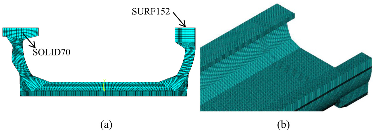
Finite element model of a U-shaped girder: (a) sectional view and (b) detail view.

Figure 5.

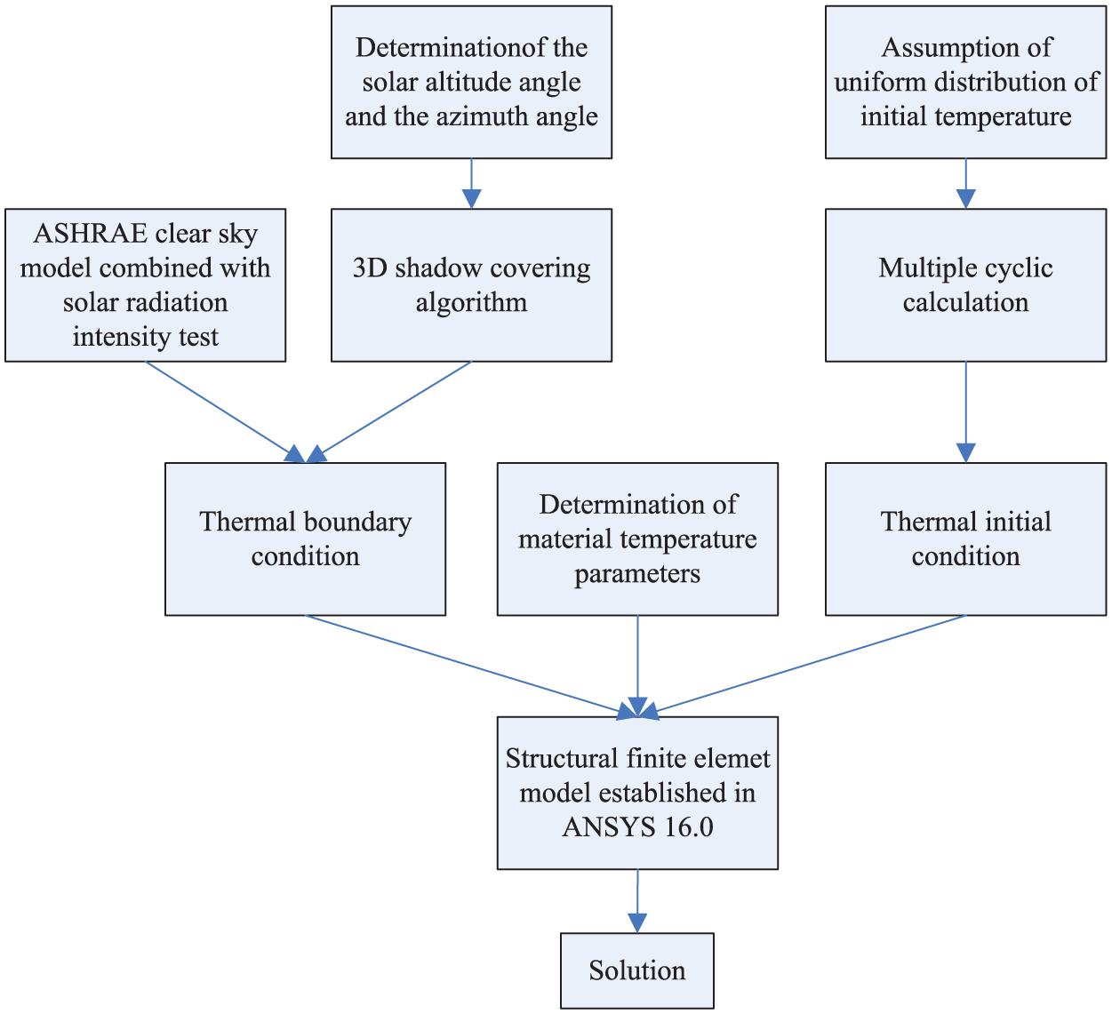
Process of numerical calculation of the 3D temperature field under solar radiation.

3D shadow covering algorithm

In the real situation, the structure’s solar radiation intensity will be affected by the shadows generated both by the structure itself and by surrounding shelters. A ray tracing algorithm was developed to calculate the real-time 3D distribution of the structural shadow in sunshine.

To implement this algorithm, the sun’s trajectory is first simulated according to the solar altitude angle $β$ and the solar azimuth angle $α$ determined in equations (4) and (5), respectively. A ray from the interface between the structure’s surface and the air is then generated according to the angle of the sun’s incident light. If the ray does not intersect with the other surfaces, direct radiation can be received by the structure’s surface; otherwise, direct radiation is obscured.

Figure 6 presents a sketch map of the algorithm implementation process. To improve the computational efficiency, the finite element model’s space was divided into several cells, and rapid intersection computation was performed with the fast traversal algorithm. Figure 6 shows that ray I emitted from plane A intersects with other surfaces in grid (4, 7), so direct radiation cannot be received by plane A. In contrast, plane B can receive direct radiation because ray II emitted from plane B does not intersect with the other surfaces within the grid.

Figure 6.

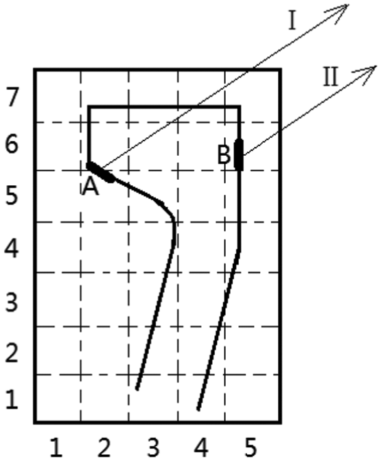
Sketch map of the ray tracing algorithm.

Case study

To verify the accuracy of the proposed method, a U-shaped prestressed concrete bridge with a span of 30 m, which has been adopted as the standard size for urban rail transit projects in Qingdao, was selected for numerical simulation and field measurements. The U-shaped girder was an open-section member with a height of 1.8 m and a width of 5.42 m. The U-shaped girder was prefabricated and placed in a clear place in the factory for temperature measurements before it was taken to the construction site. Table 1 lists the main parameters.

The atmospheric temperature is determined according to data from meteorological administration (Table 1). The conduction and convection within the air are not taken into consideration as their influence can be omitted compared with other boundary conditions presented in Figure 1.

Temperature sensors with a measurement range of −20°C to 120°C and a sensitivity of 0.1°C were installed on both the inside and the surface of the mid-span section of the U-shaped girder to record the temperature in real time (see Figure 7). The sensors installed inside the structure were assembled on the inner steel bar before concrete was poured, and the sensors on the structure’s surface were glued to the concrete surface with an epoxy resin adhesive. The acquisition, storage, and transmission of temperature data were conducted through the corresponding integrated collection box, which had a collection interval of 10 min and worked without interruption 24 h per day.

Figure 7.

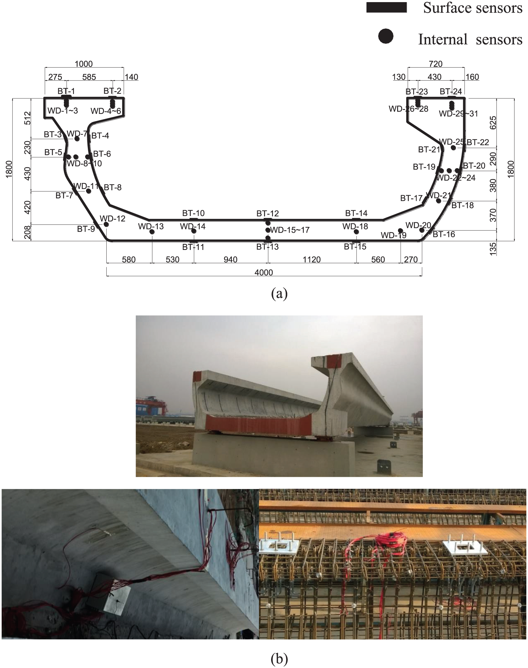
Installation of temperature sensors: (a) section view (unit: mm) and (b) photograph.

A solar radiation intensity test was conducted to verify and modify the values of undetermined parameters in the ASHRAE clear-sky model. A TBS-YG5 fully automatic tracking solar radiation detection system (Jinzhou Sunshine Meteorological Science and Technology Co., Ltd) was used to collect the solar radiation intensity data, as shown in Figure 8. This system automatically observed and preserved parameters such as the direct solar radiation intensity, the diffuse solar radiation intensity, and the solar altitude angle.

Figure 8.

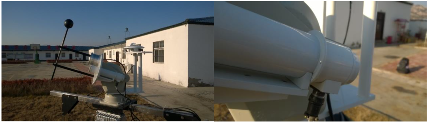
Test device for solar radiation intensity.

Updating of parameters in ASHRAE model

Figure 9 compares the measured direct radiation intensities with those predicted by the theoretical model expressed in equation (7), and Figure 10 illustrates the corresponding diffuse radiation intensities. Figure 9 shows that the predicted direct radiation intensities agree well with the measured data, but Figure 10 shows large differences between the predicted diffuse radiation intensities and the measured one, mainly because the parameter C (i.e. the ratio of diffuse radiation to direct radiation; see equation (8)) in Qingdao differs from that in the ASHRAE model. To quantify the diffuse parameter C suitable for Qingdao, the least-squares method is used to fit the measured diffuse radiation intensities. Figure 11 gives the values of the fitted parameter C in Qingdao from January to October 2015 with those from the ASHRAE model (McQuiston, 1989) and the Beijing model (Li, 1998). It can be observed that the values of parameter C significantly depend on regions and seasons.

Figure 9.

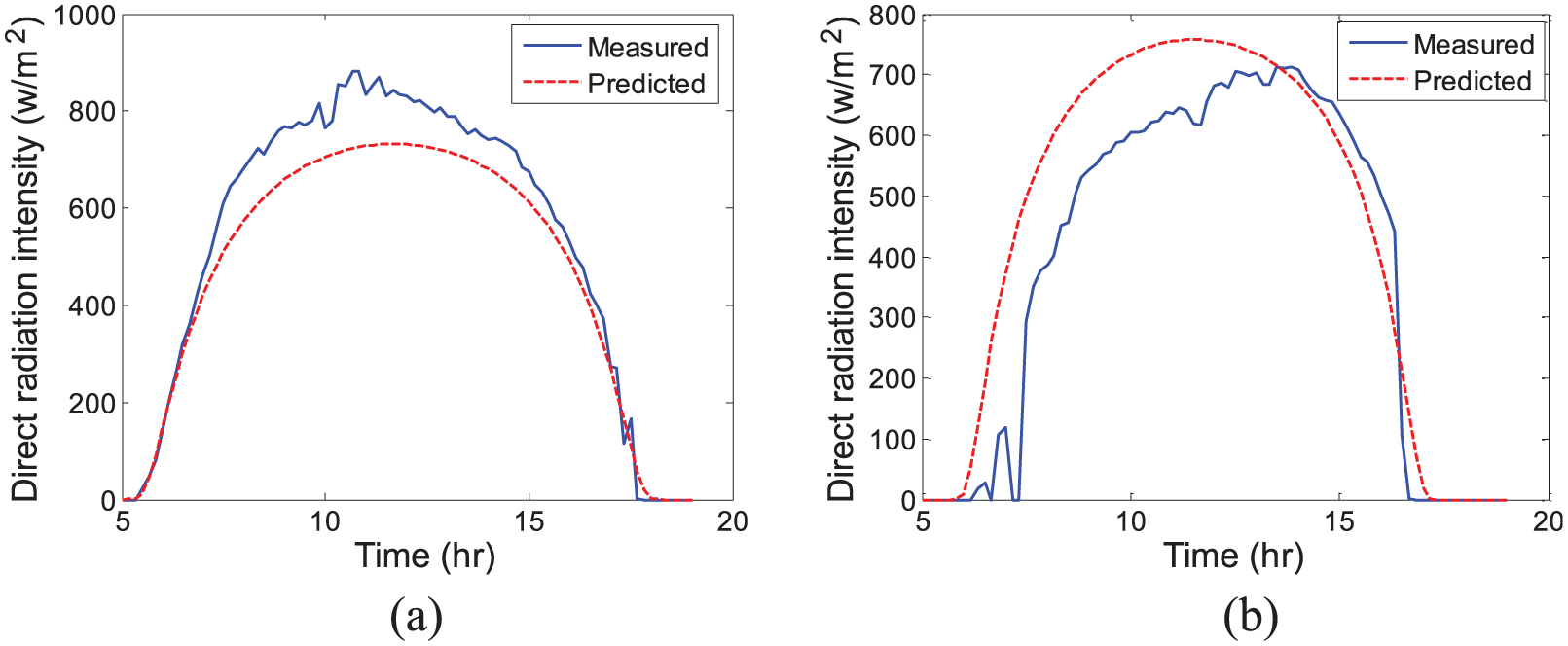
Comparison between measured and predicted direct radiation intensity: (a) 22 April 2015 and (b) 5 October 2015.

Figure 10.

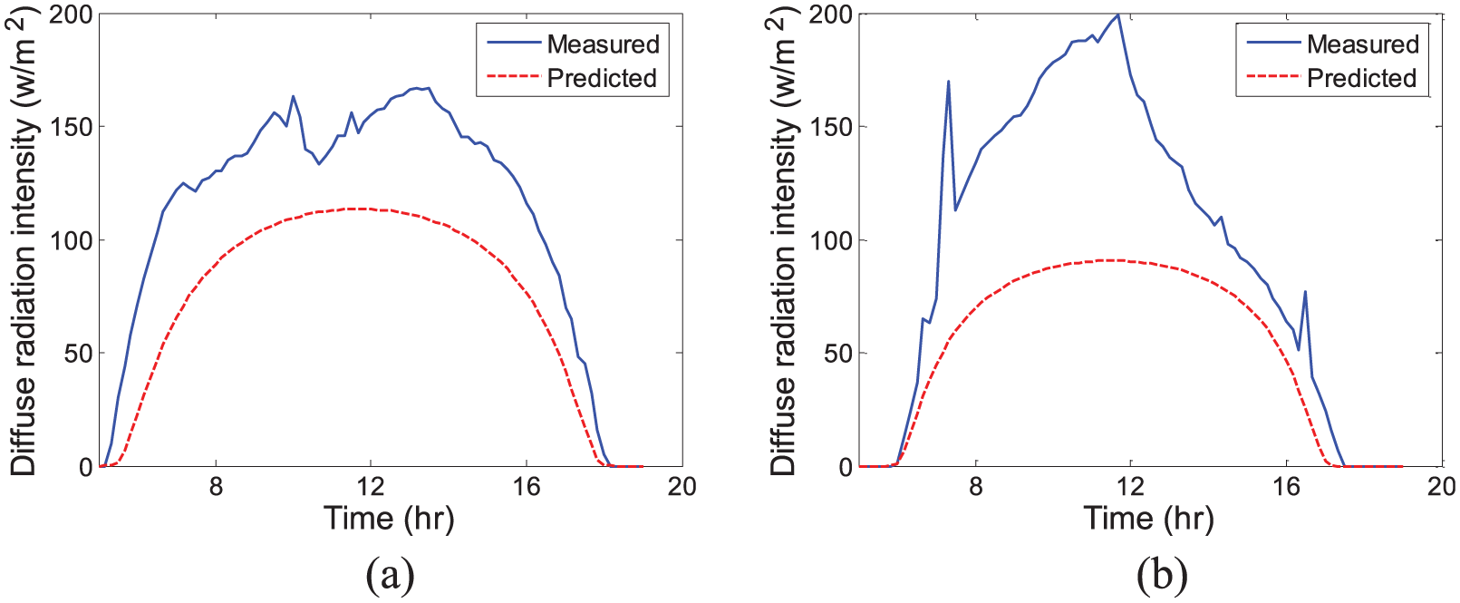
Comparison between measured and predicted diffuse radiation intensity: (a) 22 April 2015 and (b) 5 October 2015.

Figure 11.

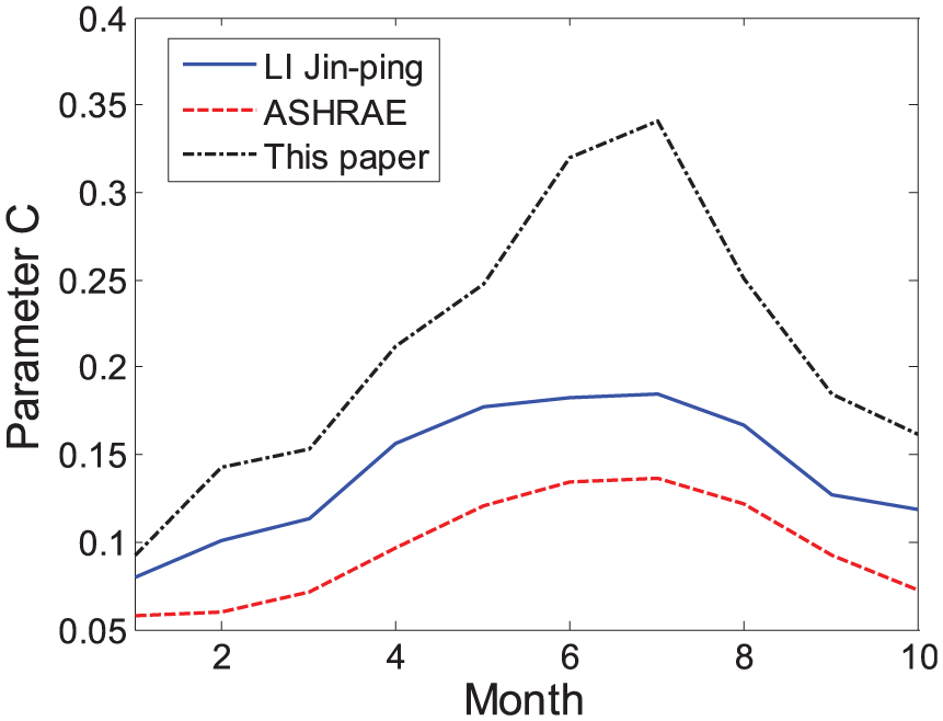
Comparison of parameter C from different literatures.

Verification of numerical simulation

The shadows on the structures have an important effect on the simulated temperature field. Figure 12 shows the calculated shadows on the U-shaped girder at various times on 14 July 2015. The parts shown in white in Figure 12 represent shadows. Figure 12(d) shows that the shadow distribution has distinct 3D characteristics at 18:00 when the solar altitude angle is low.

Figure 12.

Sketch map of calculated 3D shadow at different times: (a) 07:00, (b) 12:00, (c) 15:00, and (d) 18:00.

The initial conditions for the temperature simulation are difficult to determine, but their influence can be eliminated. Figure 13 compares the measured and predicted temperature variations during five consecutive sunny days at the measured position WD-15 on the U-shaped girder. In the calculation, the initial temperature of the U-shaped girder was set to 20°C. The calculation results on the fifth day are almost identical to the measured results, which indicates that the errors caused by the assumed initial conditions can be eliminated with a sufficient simulation time.

Figure 13.

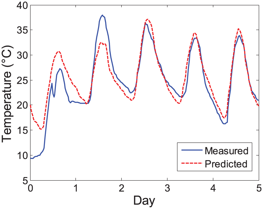
Comparison between predicted and measured temperature at measured position WD-15 during five consecutive sunny days.

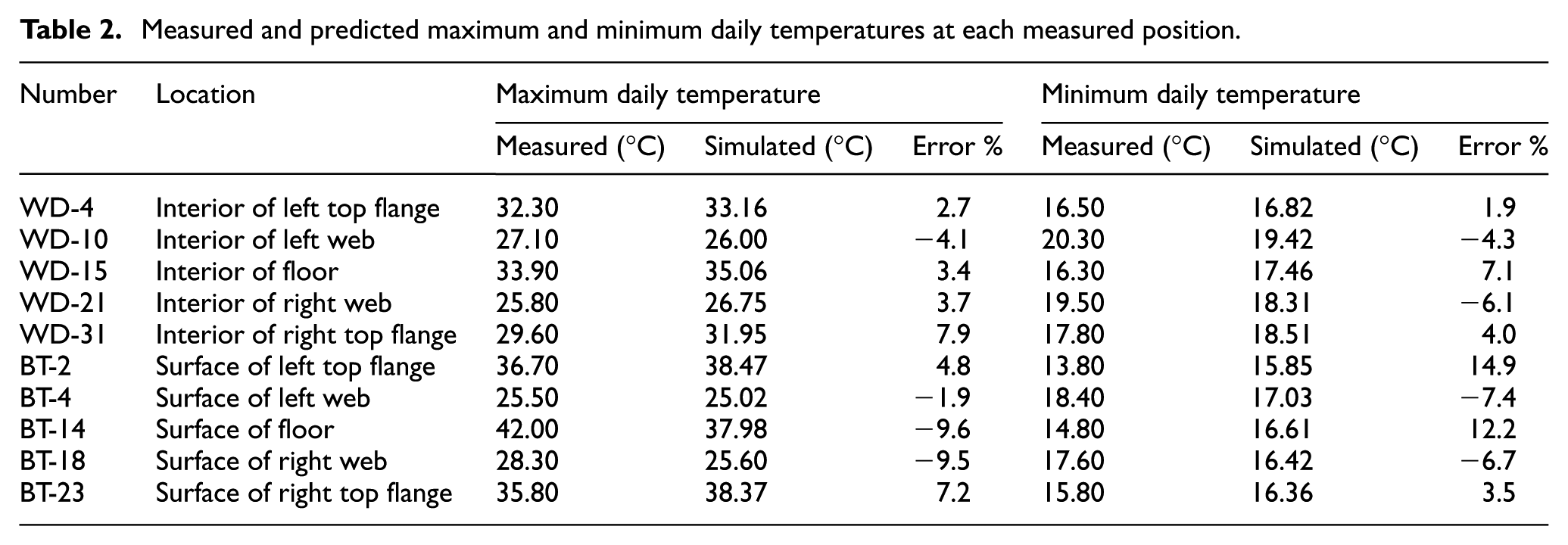
With the computed boundary and the assumed initial conditions, the temperature field of the U-shaped girder was simulated for five consecutive sunny days. Figure 14 compares the measured and predicted temperatures at measured positions WD-4, WD-21, BT-4, and BT-18 on 16 May 2015. Table 2 lists the measured and predicted maximum and minimum daily temperatures at each measured position. The computed temperature results for measured positions WD-1 through WD-31 inside the structure all agree well with the measured results, with deviations of less than 2.35°C (i.e. a 7.9% error). The differences between the simulated results and the measured results are much more significant for measured positions BT-1 through BT-24 on the structure’s surface. One reason is that the surface temperature cannot be accurately measured due to interference from the atmospheric temperature, wind speed, and other factors on the structure’s surface. In general, the predicted results are in good agreement with experimental measurements, so the numerical calculation method proposed in this article was used in the following study to obtain the structure’s detailed temperature field distribution.

Figure 14.

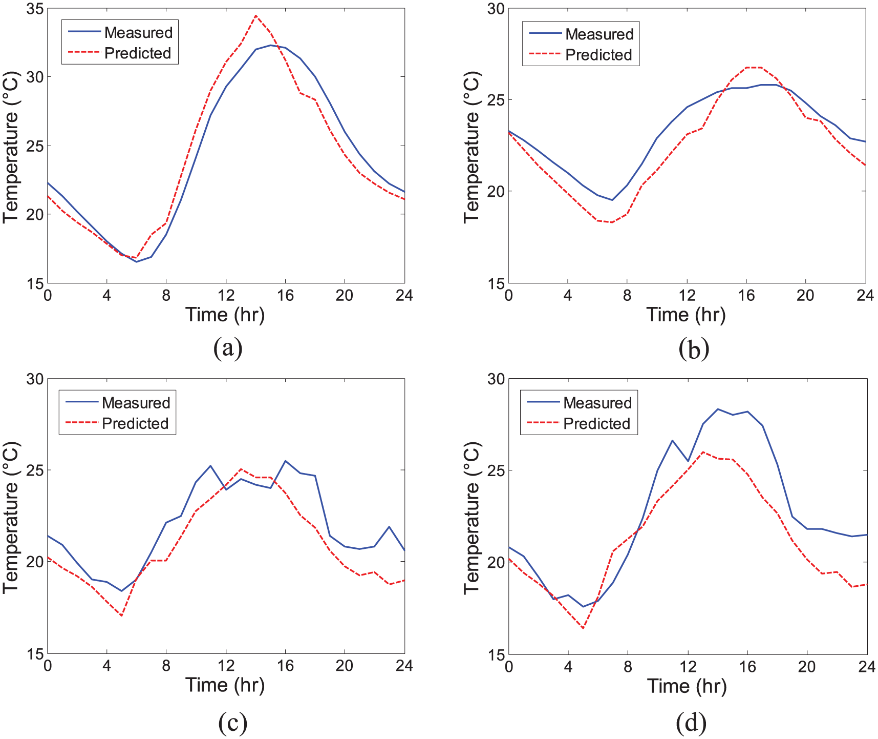
Comparison between measured and predicted temperature at various measured positions: (a) WD-4, (b) WD-21, (c) BT-4, and (d) BT-18.

Table 2.

Measured and predicted maximum and minimum daily temperatures at each measured position.

Number	Location	Maximum daily temperature			Minimum daily temperature
Number	Location	Measured (°C)	Simulated (°C)	Error %	Measured (°C)	Simulated (°C)	Error %
WD-4	Interior of left top flange	32.30	33.16	2.7	16.50	16.82	1.9
WD-10	Interior of left web	27.10	26.00	−4.1	20.30	19.42	−4.3
WD-15	Interior of floor	33.90	35.06	3.4	16.30	17.46	7.1
WD-21	Interior of right web	25.80	26.75	3.7	19.50	18.31	−6.1
WD-31	Interior of right top flange	29.60	31.95	7.9	17.80	18.51	4.0
BT-2	Surface of left top flange	36.70	38.47	4.8	13.80	15.85	14.9
BT-4	Surface of left web	25.50	25.02	−1.9	18.40	17.03	−7.4
BT-14	Surface of floor	42.00	37.98	−9.6	14.80	16.61	12.2
BT-18	Surface of right web	28.30	25.60	−9.5	17.60	16.42	−6.7
BT-23	Surface of right top flange	35.80	38.37	7.2	15.80	16.36	3.5

Distribution of the temperature field

As mentioned above, the U-shaped girder was prefabricated in the factory for the temperature measurements. The rail-bearing blocks and the rail were constructed after the girder was erected at the construction site, so only the temperature of the concrete girder was measured in a clear place at the factory. For the following discussion, the rail and the rail-bearing blocks were modeled to simulate the actual temperature field to allow investigation of the track-bridge interaction due to daily temperature variations. Table 1 lists the rail’s material properties, and Figures 15 to 17 illustrate the distribution of the structural temperature field in terms of 3D, 2D, and one-dimensional (1D) diagrams.

Figure 15.

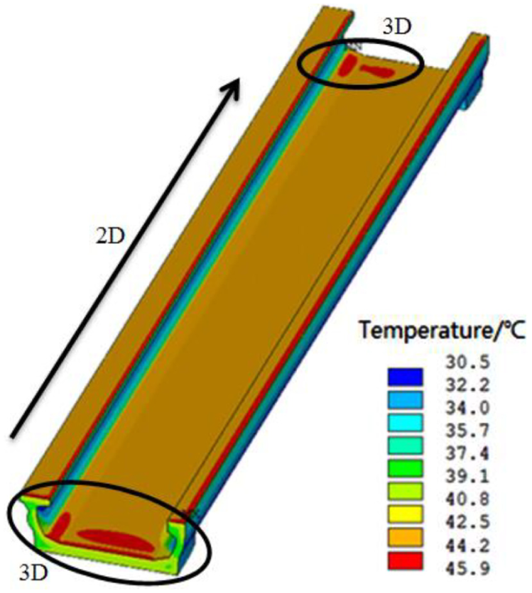
An overview of the temperature distribution of the U-shaped girder at 10:00 on 14 July.

Figure 16.

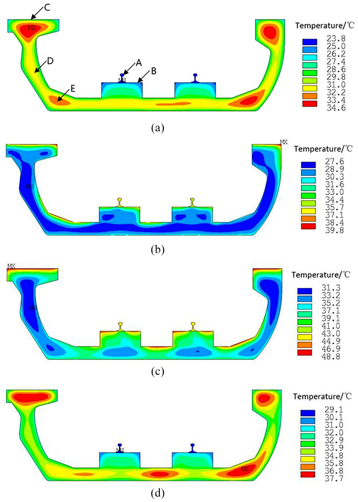
Temperature distribution of the mid-span section at typical time on 14 July: (a) 01:00, (b) 09:00, (c) 14:00, and (d) 21:00.

Figure 17.

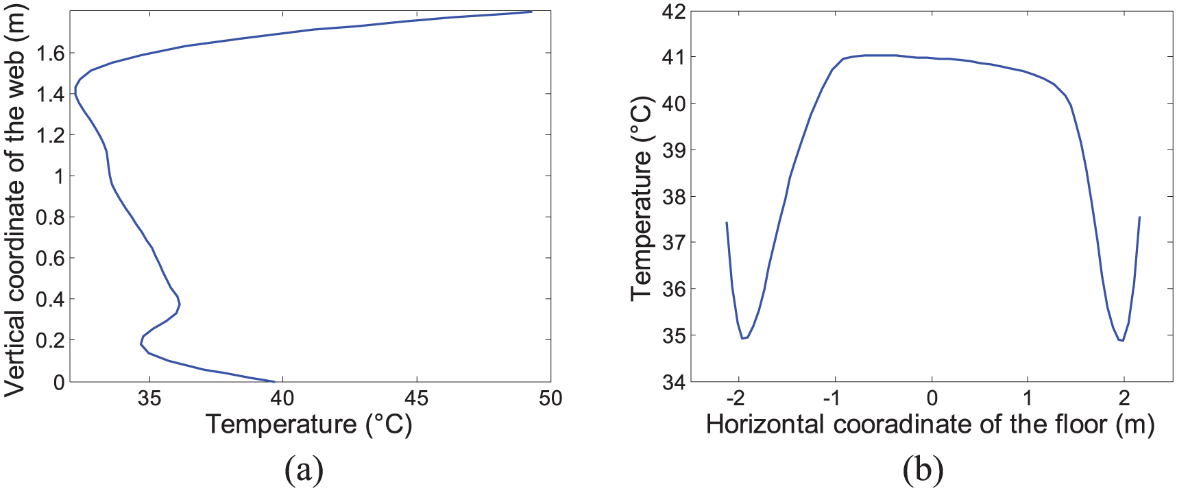
Temperature distribution curves in the mid-span section at 14:00: (a) vertical temperature distribution of the web and (b) transverse temperature distribution of the floor.

Figure 15 displays an overview of the temperature distribution of the U-shaped girder at 10:00 on 14 July. The temperature field of the rail and rail-bearing blocks was excluded from the figure to better exhibit the U-shaped girder’s temperature. Figure 15 shows that the parts of the girder surface that received direct solar radiation were about 10°C warmer than those without direct solar radiation. The temperature field has obvious 3D characteristics at the ends of the U-shaped girder, whereas it varies little along the longitudinal direction in the middle part. Therefore, it can be concluded that for simple structures with a consistent cross section, the 2D simplified method will not lead to significant errors in the calculation of the temperature field. However, the 3D effects should be considered in the numerical simulation for complicated structures with varied sections along the longitudinal axis.

Figure 16 illustrates the computed temperature field of the mid-span section at 01:00, 09:00, 14:00, and 21:00 on 14 July. Figure 16 also shows that the temperature differences within the rail cross section were insignificant due to the rail’s good heat transfer performance. The diurnal variation range of the temperature in the rail section was 23.1°C (44.7°C during the day to 21.6°C at night), which is greater than that in the concrete section. Figure 16 also shows that the temperature in the concrete section was unevenly distributed. The temperature at the surface of the concrete reached a maximum of 48.9°C at noon, but declined rapidly from the surface to the interior of the concrete. The overall temperature difference in the concrete section was about 17.5°C at 12:00. The case was exactly the opposite at night: the temperature in the interior parts of the concrete was much higher than that at the surface.

Figure 17 demonstrates both the temperature distributions of the web along the vertical direction and the temperature distributions of the floor along the transverse direction at 14:00, when the atmospheric temperature reaches its maximum. Figure 16(a) shows that the temperature on the top of the web peaks at 48.9°C and then drops rapidly to its nadir (32.3°C) within 0.36 m in the vertical direction. The temperature difference at the bottom of the web is about 5.3°C in the length range of 0.2 m. Figure 17(b) also shows that the temperature along the transverse direction of the floor first declines from the center to both sides and then rises, with a variation range of 6.0°C.

Daily temperature variation of the rail and the girder

The temperature effect plays an important role in the track-bridge interaction with continuously welded rails. The daily temperature variation of the rail and the girder has great significance in the calculation of track-bridge interaction and in its extension into structural analysis. Figure 18 depicts the variation curves of temperature during a day at several points on the rail, the girder, and the rail-bearing blocks (see Figure 16(a)).

Figure 18.

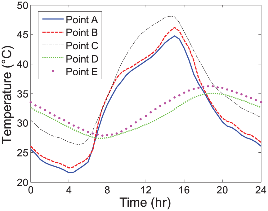
Daily variation curves of temperature at typical positions.

Figure 18 shows that the daily temperature variation curve of the rail (point A) is similar to that of the concrete at the surface of both the rail-bearing blocks (point B) and the top flange (point C), but it differs greatly from that of the concrete in the interior web (point D) and the interior floor (point E). The highest temperatures of the rail and the concrete surface range from 45°C to 48°C (at 15:00), whereas that of the interior concrete ranges from 35°C to 36.5°C (at 19:00). One reason for such a “peak lag phenomenon” might be the concrete’s low thermal conductivity. The temperature of the rail and the surface concrete grows rapidly with the increase in the ambient temperature after sunrise and peaks immediately after the ambient temperature reaches its highest. The heat conduction inside the concrete girder is much slower due to the concrete’s low thermal conductivity. As a result, it takes several hours for the temperature of the interior concrete to reach the maximum. It is also noted that the temperature variation range of the interior concrete is also smaller than that of the rail and the surface concrete.

Because the temperature in the concrete girder is unevenly distributed, the effect temperature of the girder was obtained based on the longitudinal deformation of the girder at the rail position. Figure 19 presents the variation of the temperature difference between the rail and the girder throughout the day.

Figure 19.

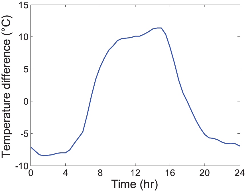
Variation of the relative temperature difference between the rail and the girder.

Figure 19 also shows that the temperature of the rail is higher than that of the concrete girder during the day. The maximum temperature difference between the rail and the girder reaches about 11.4°C at 15:00. In contrast, the temperature of the concrete girder is higher at night, and the minimum temperature difference is −8.5°C, which occurs at 01:30.

Conclusion

A self-compiled program was combined with the general finite element software ANSYS to deal with the 3D temperature boundary conditions. The solar radiation intensity was determined based on the ASHRAE clear-sky model, and the model parameters were updated according to the results of the solar radiation intensity tests. A 3D model for temperature field analysis was then proposed to include the shadowing effects and the changes in the solar radiation intensity throughout the day. Field experiments were conducted to update the established model and verify the accuracy of the numerical algorithm. The proposed method was then applied in a case study to investigate the temperature fields of both the rail and the concrete U-shaped girder. Some major conclusions can be drawn:

According to the measured data obtained from the field test, the relative errors between the numerical results and the measured results are within the reasonable range of 10%, which shows that the results are in good agreement.

With the exception of the thickened section of the girder ends, the temperature field in the concrete girder varied little along the longitudinal axis. 3D structural temperature field analysis is needed only for complicated structures with varied sections along the longitudinal axis.

Differences in temperature are insignificant within the rail cross section, but the temperature inside the concrete section has an obvious uneven distribution. The diurnal variation range of the temperature in the rail section is greater than that in the concrete section.

The rail temperature during the day is higher than that of the concrete girder, with the relative temperature difference between the rail and the girder reaching a maximum of 11.4°C after midday. At night, the temperature of the concrete girder is higher, with a minimum temperature difference of −8.5°C.

These conclusions are only applicable to selected rail-bridge systems in certain climatic conditions in specific regions. Any changes in the structural system or location may lead to different conclusions. In future studies, further verification of the relative temperature difference between the rail and the bridge can be conducted for various regions, climatic conditions, and types of concrete girders.

Footnotes

Declaration of Conflicting Interests

The author(s) declared no potential conflicts of interest with respect to the research, authorship, and/or publication of this article.

Funding

The author(s) disclosed receipt of the following financial support for the research, authorship, and/or publication of this article: This work was supported by the National Natural Science Foundation of China (No. 51278374).

References

American Society of Heating, Refrigerating, and Air Conditioning Engineers (ASHRAE) (2001) 2001 ASHRAE Handbook: Fundamentals. Atlanta, GA: ASHRAE.

Arockiasamy

Reddy

Sivakumar

et al . (2008) Fatigue loading and temperature distribution in single cell segmental box bridges. Practice Periodical on Structural Design and Construction 13: 118–127.

Barr

Stanton

Eberhard

(2005) Effects of temperature variations on precast, prestressed concrete bridge girders. Journal of Bridge Engineering 10: 186–194.

Branco

Mendes

(1993) Thermal actions for concrete bridge design. Journal of Structural Engineering 119: 2313–2331.

Churchward

Sokal

(1981) Prediction of temperatures in concrete bridges. Journal of the Structural Division 107: 2163–2176.

Elbadry

Ghali

(1983) Temperature variations in concrete bridges. Journal of Structural Engineering 109: 2355–2374.

Emerson

(1973) The Calculation of the Distribution of Temperature in Bridges. Crowthorne: Transport and Road Research Lab.

Ervine

Gillie

Stratford

et al . (2012) Thermal propagation through tensile cracks in reinforced concrete. Journal of Materials in Civil Engineering 24: 516–522.

Fleischer

Ogunbunmi

Dixon

et al . (2004) Thermal stress analysis of concrete arch dams due to environmental action. ASME 2004 International Mechanical Engineering Congress and Exposition 82: 7256–7259.

10.

Hoffman

McClure

West

(1983) Temperature study of an experimental segmental concrete bridge. PCI Journal 28: 78–97.

11.

Hunt

Cooke

Hunt

et al . (1975) Thermal calculations for bridge design. Journal of the Structural Division 101: 1763–1781.

12.

Kehlbeck

(1981) Effect of Solar Radiation on Bridge Structure. Beijing, China: Chinese Railway Publisher.

13.

Kong

Cai

Pan

(2014) Thermal field distributions of girder bridges with GFRP panel deck versus concrete deck. Journal of Bridge Engineering 19: 04014046.

14.

Lee

(2012) Investigation of extreme environmental conditions and design thermal gradients during construction for prestressed concrete bridge girders. Journal of Bridge Engineering 17: 547–556.

15.

(1998) Comparison of clear day solar radiation model of Beijing and ASHRAE. Journal of Capital Normal University 1: 37–40.

16.

McQuiston

(1989) Heating, ventilating, and air conditioning: analysis and design. Building Engineering and Systems Design 12: 379–445.

17.

Mirambell

Aguado

(1990) Temperature and stress distributions in concrete box girder bridges. Journal of Structural Engineering 116: 2388–2409.

18.

Mirza

Kaewunruen

Cong

et al . (2015) Numerical investigation into thermal load responses of railway transom bridge. Engineering Failure Analysis 60: 484–489.

19.

Moorty

Roeder

(1992) Temperature-dependent bridge movements. Journal of Structural Engineering 118: 1090–1105.

20.

Prakash

(1986) Temperature distribution and stresses in concrete bridges. ACI Journal 83: 588–596.

21.

Priestley

MJN

(1978) Design of concrete bridges for temperature gradients. Journal of American Concrete Institute 75: 209–217

22.

Ryjáček

Vokáč

(2014) Long-term monitoring of steel railway bridge interaction with continuous welded rail. Journal of Constructional Steel Research 99: 176–186.

23.

Wen-shuo

Gong-lian

Shao-chen

(2014) Numerical calculation on solar temperature field of a cable-stayed bridge with U-shaped section on high-speed railway. Journal of Central South University 21: 3345–3352.

24.

Xiong

Wen

(2014) Thermal fields of cracked concrete members in fire. Fire Safety Journal 66: 15–24.

25.

Xia

Chen

Zhou

et al . (2013) Field monitoring and numerical analysis of Tsing Ma suspension bridge temperature behavior. Structural Control & Health Monitoring 20: 560–575.

26.

Chen

et al . (2010) Monitoring temperature effect on a long suspension bridge. Structural Control & Health Monitoring 17: 632–653.

27.

Vallée

Keller

(2008) Modeling of thermal responses for FRP composites under elevated and high temperatures. Composites Science and Technology 68: 47–56.

28.

Zuk

(1965) Summary Report on Thermal Stresses in Highway Bridges. Charlottesville, VA: Virginia Highway Research Council.