
Abstract
Time-varying parameter identification is an important research topic for structural health monitoring, performance evaluation, damage diagnosis, and maintenance. Practical civil engineering structures usually contain multiple degrees of freedom; however, damage often locally occurs. In this study, a discrete wavelet transform and substructure algorithm is presented for tracking the abrupt stiffness degradation of shear structures. A substructure model is built by the extraction of the local structure which may contain damaged region. Time-varying stiffness and damping are expanded into multi-scales using discrete wavelet analysis. An optimization method based on Akaike information criterion is introduced to select the decomposition scale. The expanded scale coefficients are evaluated using least square method, then the original time-varying stiffness or damping parameter is identified by reconstructing from the scale coefficients. To validate the proposed method, a numerical example of seven-story shear structure with time-varying stiffness and damping is proposed. Experiment for a three-story shear-type structure with abrupt stiffness degradation is also tested in the laboratory. Both numerical and experimental results indicate that the proposed method can effectively identify the abrupt degradation of stiffness parameter with a satisfactory accuracy.
Introduction
Parameter identification of civil engineering structures is an important research topic, and most of the parameter identification techniques are focused on time-invariable systems. However, many practical civil engineering structures exhibit time-varying characteristic during their operation period due to the environmental erosion, material aging, load effect, and structural damage. It is significant to identify time-varying parameter for structural health monitoring, performance evaluation, damage diagnosis, and maintenance.
When damage occurred, structure is usually deemed as a nonlinear system. Some studies focused on the parameter identification of nonlinear system. Wu and Smyth (2007) applied the unscented Kalman filter (UKF) technique for real-time nonlinear structural system identification and compared the extended Kalman filter (EKF) with UKF for nonlinear structural system identification. Xu et al. (2012a) presented an iterative approach named weighted adaptive iterative least squares estimation with incomplete measured excitations (WAILSE-IME) for both structural parameters and dynamic loading identification. A date-based model-free identification method was proposed for identifying structural hysteretic restoring force and mass with incomplete external excitations (Xu et al., 2015). Xu and He (2015) introduced a time-domain substructural identification method by combining a weighted adaptive iteration algorithm and an EKF approach for identifying structural physical parameters and dynamic loading. Yan and Katafygiotis (2016) applied transmissibility matrix, random matrix, and substructure technique to stochastic system identification.
Some techniques have been proposed for the identification of time-varying modal parameters, for example, the state-space method (Weng and Loh, 2011; Xu, et al., 2012b), the Hilbert–Huang transform (HHT) (Shi et al., 2009), the wavelet transform (Dziedziech et al., 2015; Shan and Burl, 2011; Su et al., 2014; Wang et al., 2013), and time–frequency analysis method (Kougioumtzoglou and Spanos, 2013; Pai, 2010; Wang and Chen, 2012). However, structural damage usually reflects the variation of physical parameter, such as stiffness and damping. Identifying the time-varying physical parameter is more directly for structural damage diagnosis. Accordingly, some physical parameter–identifying techniques have been proposed.
One type of identifying techniques was based on subspace theory. Liu and Deng (2004) proposed a subspace method and built a cantilever beam experiment to validate the presented method. Pang et al. (2005) proposed an improved algorithm based on the whole data subspace, which enhanced the anti-noise of the identified method. Li and Shi (2008) proposed a subspace method to identify time-varying physical parameter based on stochastic force response. Jing and Liu (2007) presented an online parameter identification method to identify physical parameters at joints in a moving structure.
The other type of method was based on the online recursion technique. Loh et al. (2011) and Yang and Lin (2005) proposed a different online recursion subspace algorithm with adaptive forgetting factor. Yang et al. (2006) proposed an improved Kalman filter identifying technique by replacing the forgetting factor variable with an adaptive factor matrix. Bisht and Singh (2014) proposed an adaptive unscented Kalman filter approach for tracking the structural time-varying stiffness. Lei et al. (2016) proposed a time-domain three-stage algorithm based on extended Kalman filter for real-time tracking of the abrupt stiffness degradations of structural elements. These methods were successfully applied to different types of time-varying structures, in various cases; however, the computation work was time-consuming because the adaptive factor had to be updated at each time instant by optimizing.
In addition, HHT-based identifying methods have also been proposed by some researchers. Shi and Law (2007) developed a Hilbert transform and empirical mode decomposition (EMD) technique for the identification of time-varying system using forced vibration response time histories. Yi and Duan (2007) proposed a HHT technique for identifying structural stiffness. Wang and Chen (2013) developed a recursive HHT method for the time-varying property identification of shear-type buildings under base excitations, which allowed for the evaluation of stiffness and damping in each story step by step. However, EMD technique was empirical and was not strictly proven mathematically.
In recent years, wavelet transform as an advanced time-frequency analysis technique has been applied into the time-varying structural parameter identification. Xu et al. (2012b) proposed a wavelet-based state-space identification method. It transformed the second-order vibration differential equations into the first-order state equations using the state-space theory, and then, the state-space equations were transformed into linear equations by projecting the excitation and structural response using wavelet scaling functions. Shi and Chang (2012) proposed a time-varying parameter identification technique based on wavelet multi-resolution analysis (WMA) and substructural method, and a shear-beam experiment was carried out to validate the method. Wang et al. (2014) proposed a discrete wavelet transform (DWT)-based method for time-varying physical parameter identification for shear-type structures. The time-varying physical parameters were dispersed using discrete wavelet basis as time-invariant scale coefficients, and then, the coefficients were estimated using regular least square method.
The practical civil engineering structures usually contain many degrees of freedom (DOF); when the method based on discrete wavelet is adopted, the excessive DOFs aggravate the ill-posed problems of system identification and require more computational time. In fact, damage usually occurs in the local structure, one can use the substructure technique to decrease the dimension of the problem. In this study, a DWT and substructure algorithm is presented for tracking the abrupt stiffness degradation of a shear structure. A substructure model is built by extracting the local structure which may contain damage region. Then, the method based on discrete wavelet is applied to the substructure model to identify the time-varying parameter. The proposed method is validated by a numerical simulation of seven-story shear structure and experimental analysis of three-story structure with abruptly changing stiffness.
DWT
For finite-energy signal,
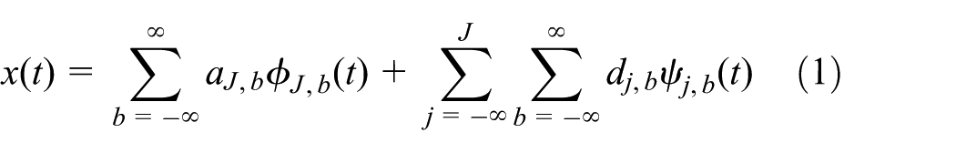
where J denotes the max decomposed scale;
For practical discrete and finite length signal x(n), it can be approximately regarded as scale coefficients a0, b at zero scale, so the discrete wavelet analysis can be defined as
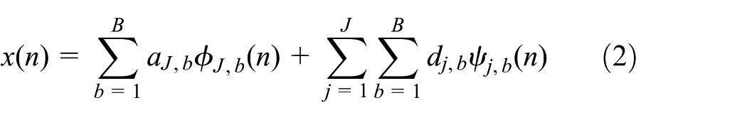
where B is the number of decomposed wavelet coefficients at different scales.
Identification method
General scheme based on DWT
As presented in Wang et al. (2014), a single-DOF shear structure with time-varying stiffness and damping is used to explain the identification method. The dynamic equation can be expressed as

where
For the practical discrete structural response, the discrete form of last equation can be expressed as

The time-varying stiffness and damping can be regarded as a discrete signal, so they can be expanded using discrete wavelet according to equation (2). For a slow time-varying signal, its main energy concentrates in the region of low frequency, so the time-varying parameter can be approximately expanded as follows
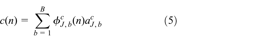
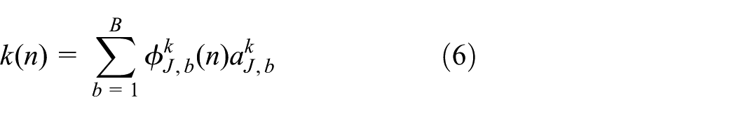
It is worth mentioning here that, in above equations, c and k involved in the superscripts are used to distinguish the decompositions corresponding to damping and stiffness, respectively.
Substituting the above equations into equation (4) and considering the scale coefficients as the unknown variable, one can obtain the transformed identification equation as

where
The unknown scale coefficients can be estimated using least square method as

By substituting the solution into equations (5) and (6), the structural time-varying damping and stiffness can be identified.
Substructural identification scheme based on DWT
Practical structures usually have many stories, certainly the abovementioned method can be extended to the multi-DOFs shear structure. However, it is needed to simultaneously measure the response of all DOFs, which is inconvenient in practice, and more DOFs may aggravate the ill-posed problem of solving equation (8). Also, the anti-noise performance of the method will become worse. Actually, the time-varying damage usually occurs in the local parts of structure; here, a method combining the DWT and substructure technique is proposed for the identification of multi-story shear structure.
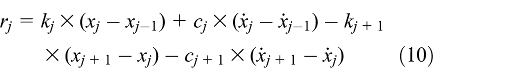
For a mutli-story structure, as shown in Figure 1, it is assumed that time-varying degradation due to load excitation during operation occurred in the s stories indexed from i+1 to i+s. According to the substructure technique proposed by Koh et al. (1991) and Trinh and Koh (2011), the local s stories can be extracted as a substructure, and the internal force on the interface between the substructure and the remaining part can be applied to substructure as external force. The dynamic equation for this substructure can be expressed as follows

where
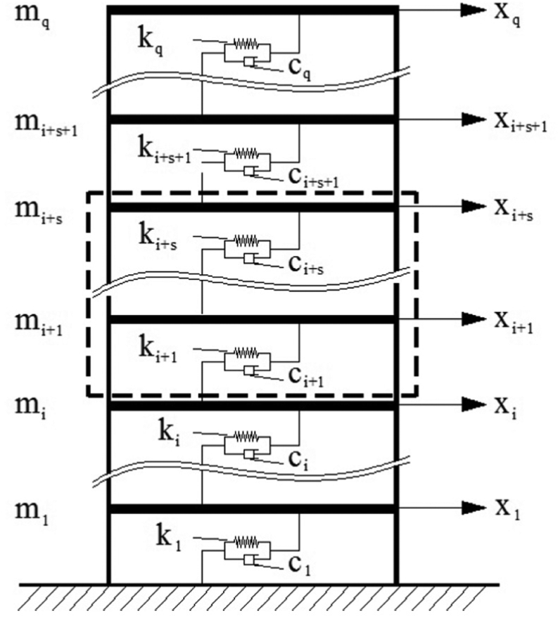
The multi-story shear structure.
where

where
Substituting equation (11) into equation (9), the dynamic equation of substructure can be transformed as

If the practical structural response is discrete sampled, the corresponding discrete form of equation (15) can be obtained by substituting the continuous time s as discrete variable n

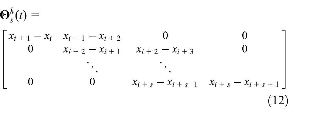
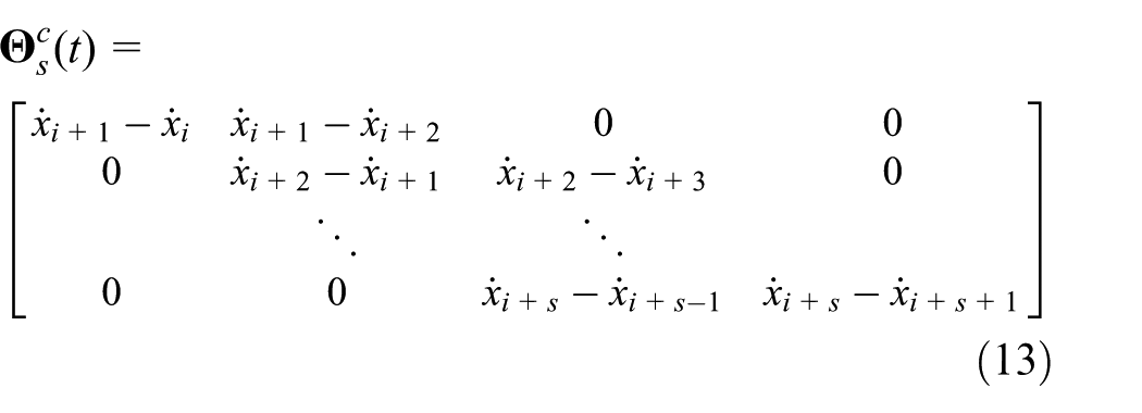
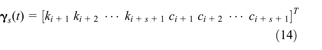
From the above deduction, it is necessary to identify
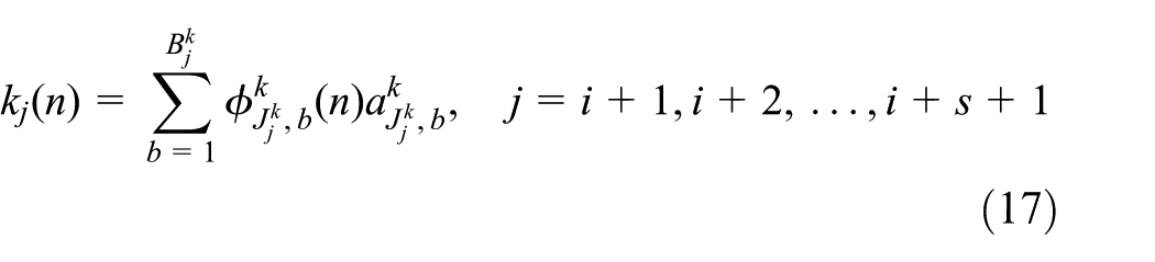
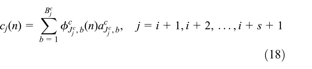
where
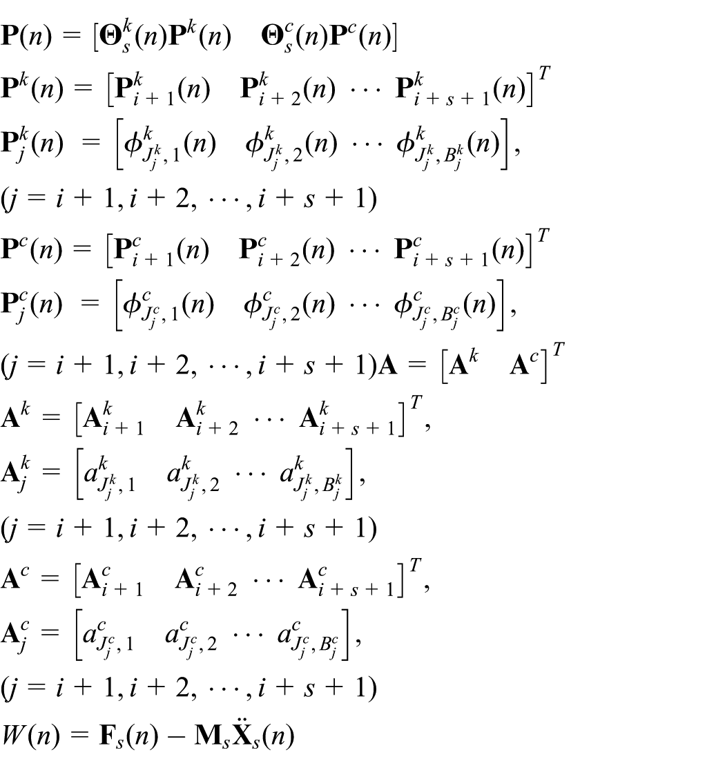
Substituting equations (17) and (18) into equation (16), one can obtain the finally identified equation as

where
In the same way, the scale coefficients can be estimated using least square method as follows

So, the time-varying parameters can be identified by substituting the solved result into equations (17) and (18).
Parameter optimization
The decomposition scale is an important parameter for DWT. If the larger decomposition scale is selected, the less unknown scale coefficients need to be identified; however, more high-frequency components are lost when the parameter is expanded according to equations (17) and (18), which would reduce the precision of time-varying parameter reconstructed from estimated scale coefficients. On the contrary, if the small decomposition scale is selected, it will increase computational consumption due to the more scale coefficients, and the introduction of much more high-frequency components may lead to an over-fitting problem that will amplify the effect of noise.
Different decomposition scales would lead to various solution models and identification equations like equation (19), so the optimal decomposition scale can be determined by selecting appropriate model based on statistical properties of the models. Here, the Akaike information criterion (AIC) proposed by Shi and Chang (2012) is adopted.
Assuming that the decomposition scales of time-varying damping and stiffness are
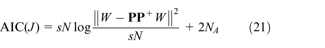
where N is the length of response signal, NA is the number of all decomposition scale coefficients in equation (19), and
The first item reflects the error of model fitted, and the second part accounts for the penalty on the number of scale coefficients listed in equation (19). Because the optimal model have minimized AIC value, the optimal decomposition scale J can be determined by solving minimize AIC.
Numerical verification
In order to validate the proposed method, a seven-story shear structure with time-varying stiffness and damping is simulated as a numerical example. The structural model is shown in Figure 1.
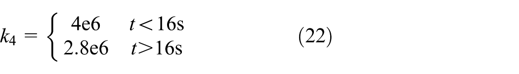
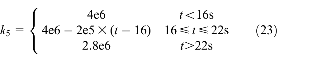
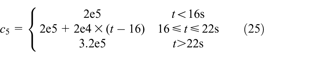
Assume that the initial parameters of model as

Assuming that the white noise force is applied on the top floor, the structural response of each floor can be solved using a fourth-order Runge–Kutta method, and the sample frequency of response is set as 50 Hz. To study the effect of noise on the proposed method, one additional case with 10% (defined as ratio of root mean square of noise and signal) Gaussian white noise is added to solve response signal for analysis.
If the DWT method is adopted directly, it is needed to simultaneously measure the response of all DOFs, which is convenient in application. And, it needs to identify the parameters of each floor. In this case, there are 14 parameters needed to be identified. Excessive identification parameters will cause to the ill-posed problem, and it will greatly increase computing consumption for optimizing wavelet parameters and equation solving. However, if the fourth and the fifth floors are extracted as a substructure, only part of response from the third to the sixth floors is required, and the parameters from the fourth to the sixth story are estimated. The required response data are shown in Figures 2 and 3.
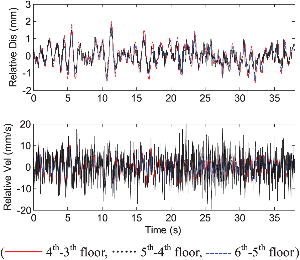
The calculated relative displacement (Dis) and velocity (Velo) of different floors (––– fourth–third floor, fifth–fourth floor, ------ sixth–fifth floor).
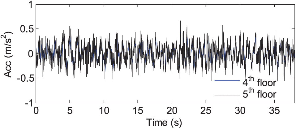
The calculated acceleration (Acc) of different floors.
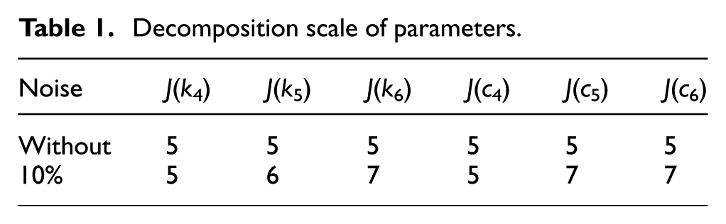
Because the stiffness and damping of fourth floor changes linearly, the “db3” wavelet is used to parameter identification, but the “haar” wavelet is selected for the sudden time-varying parameter of fifth floor and constant parameter of sixth floor. The decomposition scale of all the parameters are determined based on the AIC, and the optimized result is listed in Table 1.
Decomposition scale of parameters.
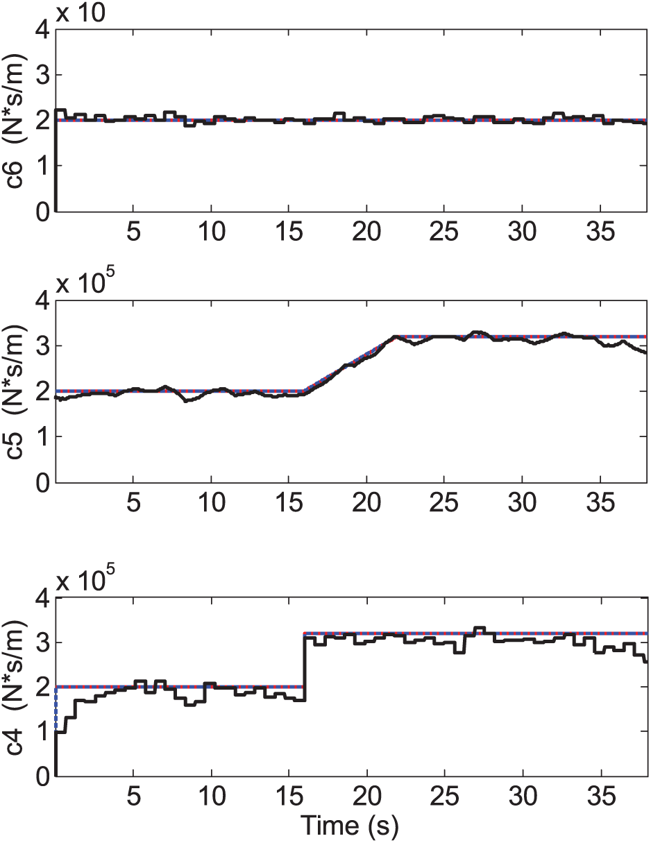
The proposed substructural method is applied to identify the time-varying parameters from the fourth to the sixth floor in two cases, and the identified results are shown in Figures 4 and 5. For comparison, the theoretical values of parameters are plotted in the same figure using a red solid line.
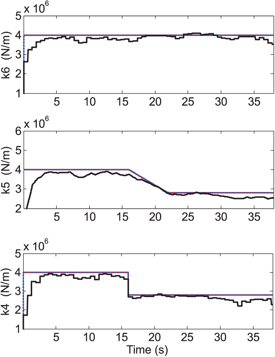
The identified stiffness (––––the theoretical value, the identified result without noise, –––the identified result with 10% noise).
The identified damping (–––––––the theoretical value, the identified result without noise, –––the identified result with 10% noise).
It can be observed that the proposed method can effectively identify the time-varying stiffness and damping with high precision in the case of without noise. When 10% Gaussian white noise is injected to the simulated responses, the identified result has some fluctuation, but it can still effectively track the variation of parameter. Only there is slightly large error at the end of time, which is mainly caused by end-effect of wavelet transform. It can be also seen that the “haar” wavelet makes good performance of catching the abruptly varying of parameter.
Experiment verification
Design of experiment
To further verify the proposed method, a three-story shear-type structure model is tested in the laboratory. The model is composed of four steel plates with the of dimensions 420 mm × 380 mm × 3 mm. Two ear plates are welded on both sides of each steel plate, through which some springs can be installed between the two floor steel plates. And, a small quadrate block is welded on middle of lateral of each steel plate as a joint of connecting external load. Each two stories are bolt-connected by four columns of dimensions 323 mm × 22 mm × 2 mm. Three types of sensors are installed on every floor to measure the horizontal acceleration, velocity, and displacement. The acceleration sensor is fixed on the plate by small magnet, and the velocity sensor is settled using plasticine. As for the measurement of displacement, a magnetostrictive type of sensor is adopted. Only a magnetic ring is bolt-connected on the steel plate, the measuring rod crossing the ring is not in contact with the model, which is fixed on an independent steady. For applying exciting force to the model, a vibration exciter is connected to the top floor of the model by a magnet, and a force sensor is installed between the vibration rod and connected magnet to measure the force.
For simulating the abrupt changing of structural stiffness, two springs are installed between the first and the second floor of the steel plate. First, four electromagnets are fixed on ear plates of upside of the first floor and downside of the second floor, respectively. Then, two small steel blocks are connected onto both ends of each spring, and the whole mass of one spring and two steel blocks is 0.335 kg. Turning on the power of electromagnets, the springs on the model can be installed by connection with steel blocks and electromagnets. When the power is turned off, the springs will depart from the structural model, which will induce a sudden variation in the second floor stiffness. The connecting construction of spring is shown in Figure 6.
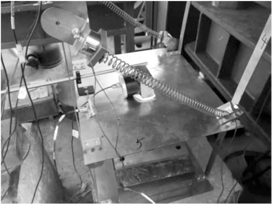
The connecting construction of the spring.
The mass of all the components including steel plate, sensors, columns, electromagnetic, and so on are measured first. The mass of columns is distributed to adjacent story according to the lumped mass method, without the mass of spring; the measured mass of every floor except ground floor from bottom to top is defined as m1 = 5.994 kg, m2 = 5.994 kg, and m3 = 5.541 kg. The whole experiment model is placed on a concrete block, and the ground floor is fixed by weight blocks as foundation. The experimental setup of time-varying frame model is shown in Figure 7.
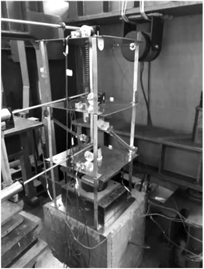
The experimental setup of time-varying frame model.
Three cases of dynamical experiment are carried out, which are as follows:
Case A: no springs are installed on the model and the model is time-invariant.
Case B: a couple of springs are installed between the first and second floors by electromagnet, and the power of electromagnet is turned on during the experiment, so the model is still time-invariant.
Case C: at the beginning of the experiment, two springs are connected between the first and second floors. During the vibration of the model, the power of electromagnet is turned off and simultaneously the springs depart from the model, so the stiffness of structure is time-varying.
In all cases, the white noise signal is inputted into the vibration exciter, and the generated force is applied to the top floor of the model. The exciting force and structural response including acceleration, velocity, and displacement will be measured simultaneously, and the sampling frequency is 100 Hz.
Test of stiffness
To verify the identified effect of promoted method, the horizontal stiffness of each floor is first tested using static method. Comparatively speaking, static test has been widely viewed as a more straightforward method, and it is of higher accuracy than the dynamics-based approach as the latter is less robust due to various effects. First, the frame model is assembled. On the horizontal position of the first floor steel plate, a dial indicator is installed on the middle of one side to measure its horizontal displacement. On the other side of the steel plate, a rope across a pulley is tied on the model. By adding a weight on the other end of the rope, a horizontal pull is applied to the model. In this test, a small steel plate with mass of 1.225 kg is hanged on the rope as load. The static test setup of horizontal stiffness is shown in Figure 8.
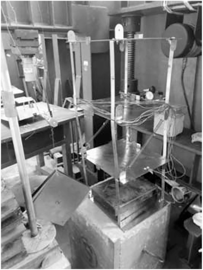
The static test setup of horizontal stiffness of model.
By increasing the number of hanged steel plates and measuring the corresponding displacement of the first floor, its horizontal stiffness based on the curve between tension and displacement can be calculated. After the test of the first floor was finished, the dial indicator and load system was moved to the position of the second floor to measure its stiffness. For the stiffness of the second floor, two cases, with spring and without spring, are tested. The same process is carried out to the third floor.
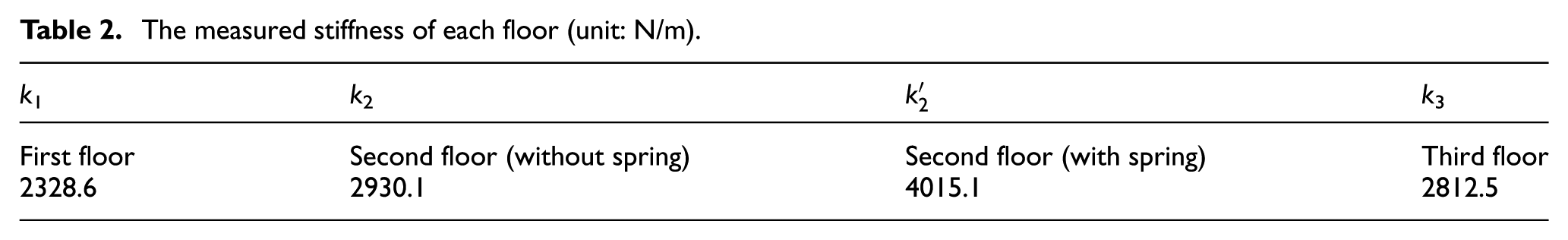
The structural stiffness can be obtained using least square linear fitted with the data of tension and displacement. Partial tested curves of tension and displacement of the first and second floors are shown as Figure 9, respectively; the measured value is plotted by symbol “*.” And, the tested stiffness is shown in Table 2.
The measured stiffness of each floor (unit: N/m).

The curve of tension and displacement: (a) first floor and (b) second floor.
Stiffness identification
The experimental model was approximately simulated as a 3-DOF shear-type structure. Its dynamic equation is as similar to equation (5). For each case, the stiffness and damping are considered as unknown time-varying parameters which are needed to be identified. If the DWT method is adopted directly, all the response and exciting force need to be used. However, if the proposed substructure identification method is adopted, the first and second floors can be extracted as substructure. In this case, only part of structural response and the exciting force are unnecessary. For comparing their effect, both methods are adopted to identify the parameter. For case A, the measured displacement, velocity, and acceleration of second floors are shown in Figure 10.
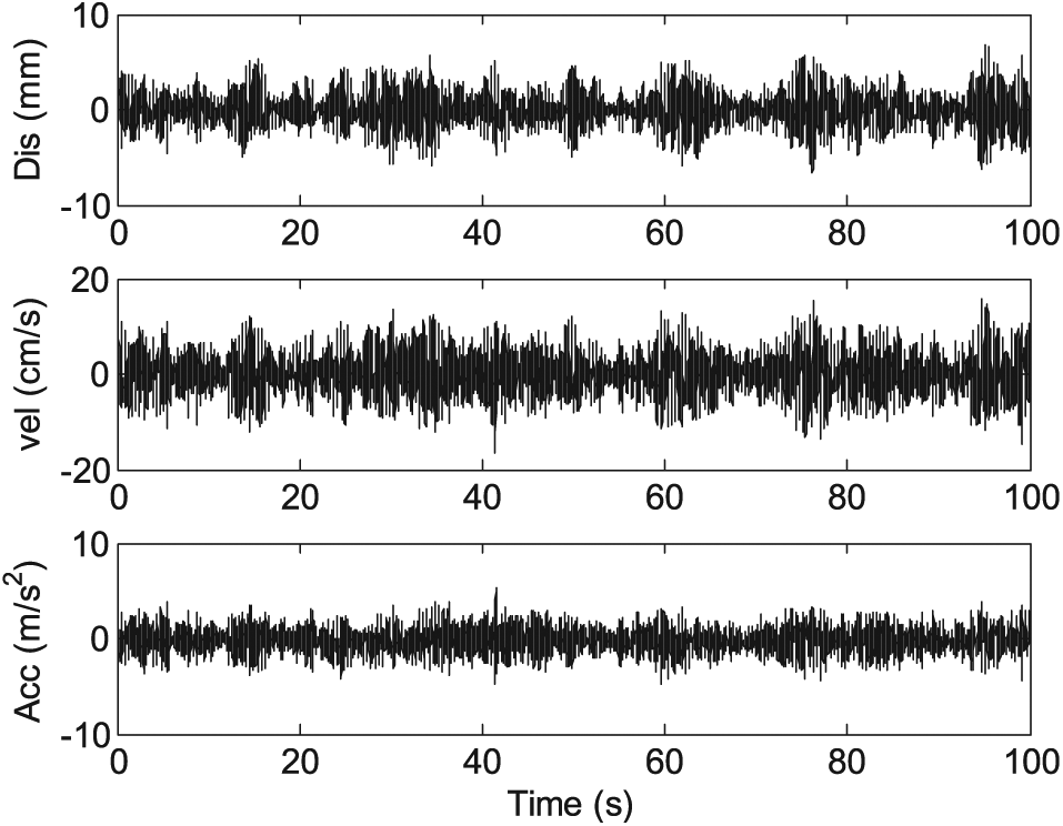
The measured displacement (Dis), velocity (Vel), and acceleration (Acc) response of the second floor.
The “haar” wavelet is adopted due to the abruptly varying stiffness. The decomposition scale of parameters is optimized based on AIC approach, and the optimized result is shown in Table 3.
Decomposition scale of parameters.
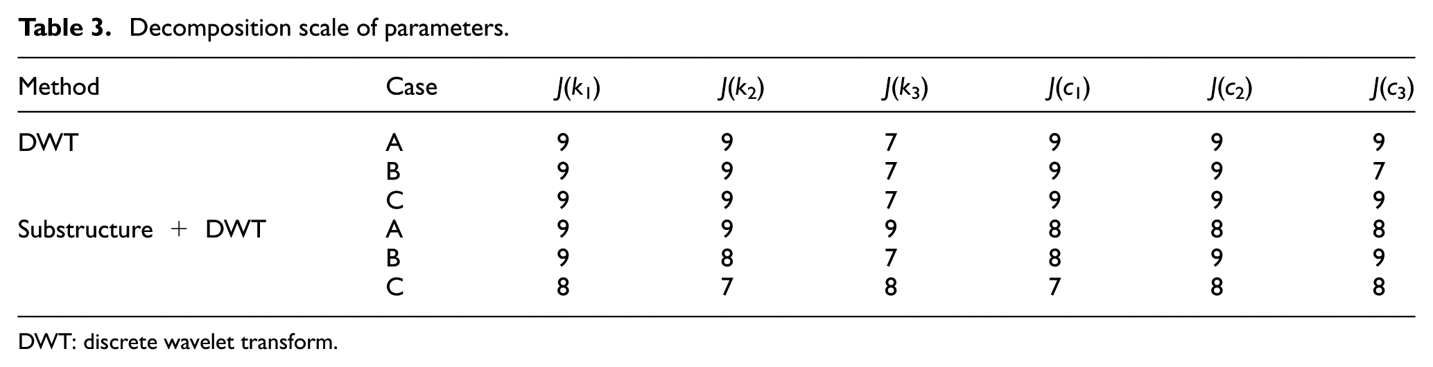
DWT: discrete wavelet transform.
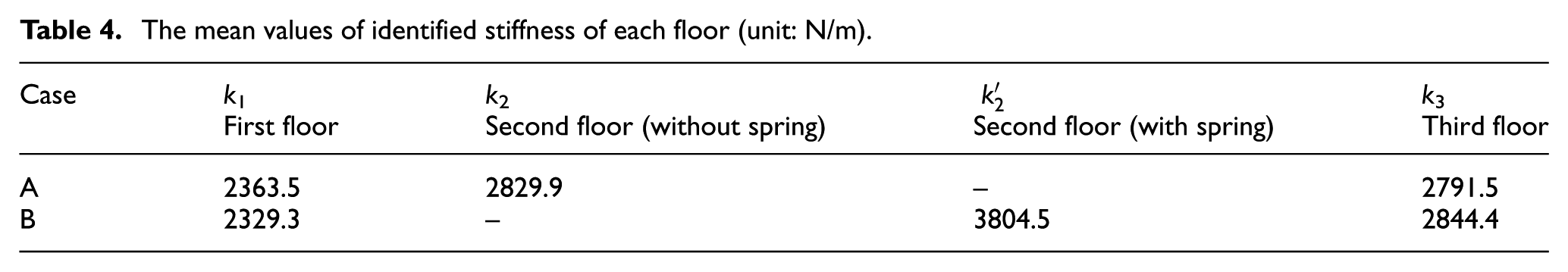
Two methods (based on DWT and based on substructure and DWT) are used to analyze the experiment data of case A and B. Since it is difficult to obtain the theoretical damping result for comparison, only the identified stiffness result is presented in Figures 11 and 12, and the measured stiffness by static test is also plotted in the same figure using a red dashed line for comparison. For the quantitative comparison with static test result, the mean values of identified stiffness of each floor by substructure method are listed in Table 4.
The mean values of identified stiffness of each floor (unit: N/m).
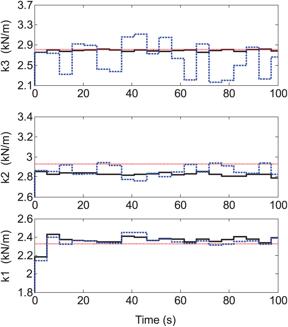
The identified stiffness in case A ( the static tested result, ---------the identified result based on DWT, ––––the identified result based on substructure and DWT).
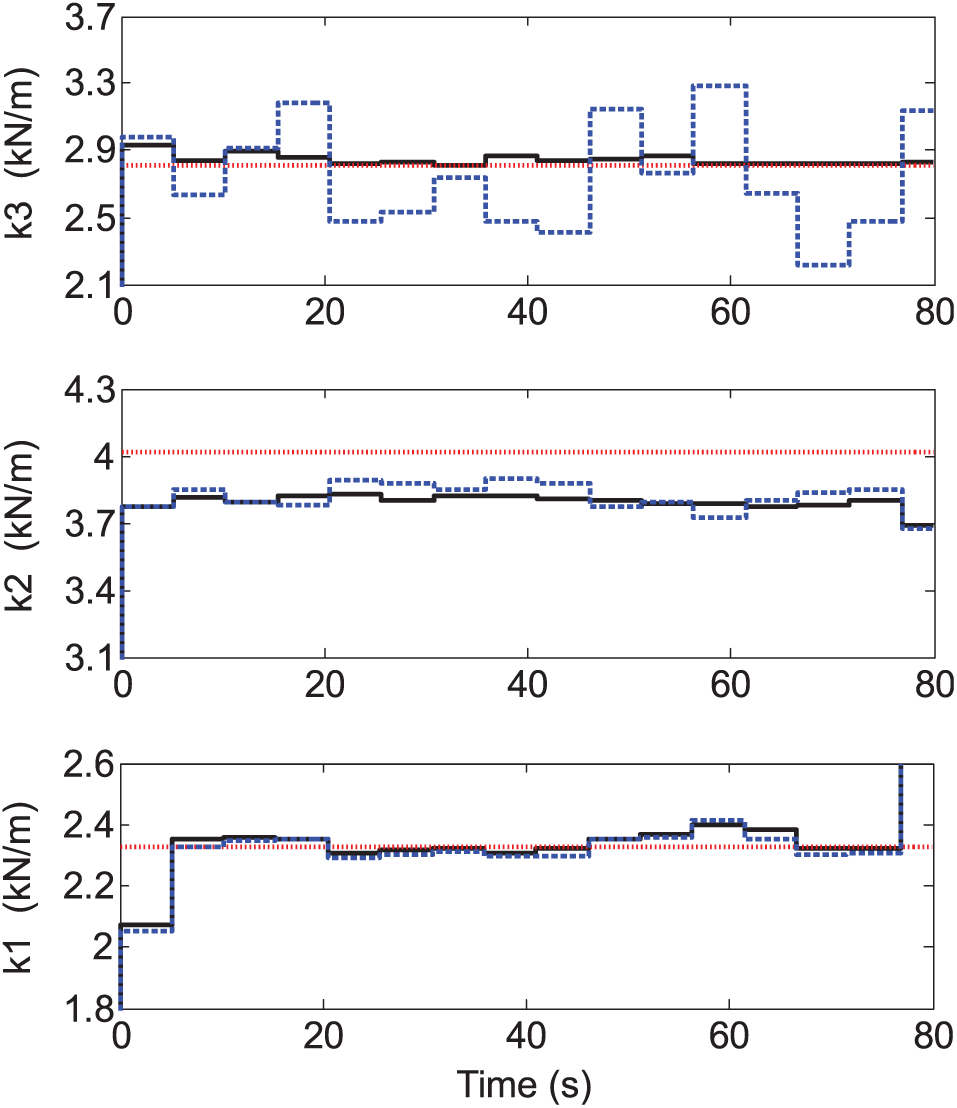
The identified stiffness in case B ( the static tested result, ---------the identified result based on DWT, ––––the identified result based on substructure and DWT).
It can be seen that the identified result based on substructure and DWT is better than that of using DWT method in both two cases. When the substructure and DWT method is adopted, the identified stiffness of the first and the third floors makes good agreement with the static test result. The slightly large error at the end of time is caused by end-effect of wavelet transform. For the second stiffness, there is an overall error between the identified and tested result, and the average deviation is about 5.2%, which is due to the deviation between the practical structure and the assumed shear-type dynamic model. For case C, the structure is time-varying, and its response and exciting force are shown in Figures 13 and 14, respectively.
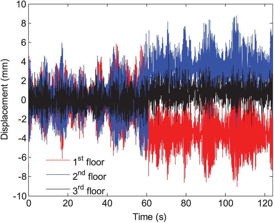
The displacement response of three floors.
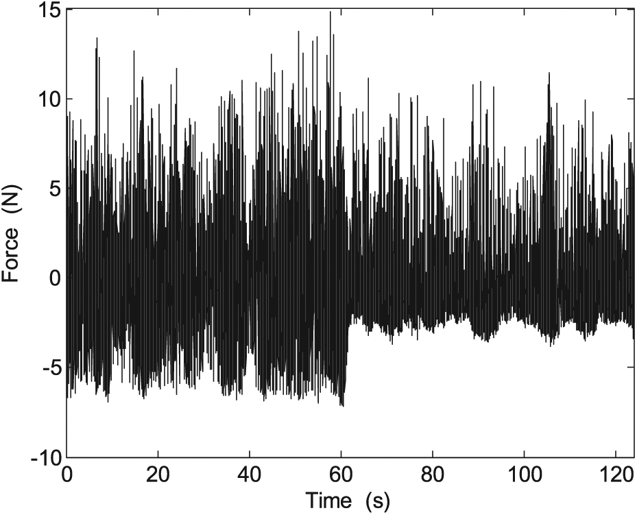
The curve of exciting force in case C.
It can be clearly seen that the structural displacement and exciting force suddenly change at about 60 s, at which time the power of electromagnet is turned off, and the spring departs from the model, so the structure reaches quickly the new balanced position and vibrates around it. In this case, the structural mass also changes because of departing spring, so it is needed to adjust the mass of model after the time of turning off power of electromagnet. The article mainly focuses the identification of stiffness, and the mass of each component has been tested in advance, so during the process of identifying the abrupt stiffness degradation, the mass of model is updated before and after the lease of the spring. The updated time point can be determined by decomposing the signal into multi-scale components using DWT. Figure 15 shows the decomposed fifth-scale approximate (marked as a5) and detail components (marked as d5) of the first floor displacement.
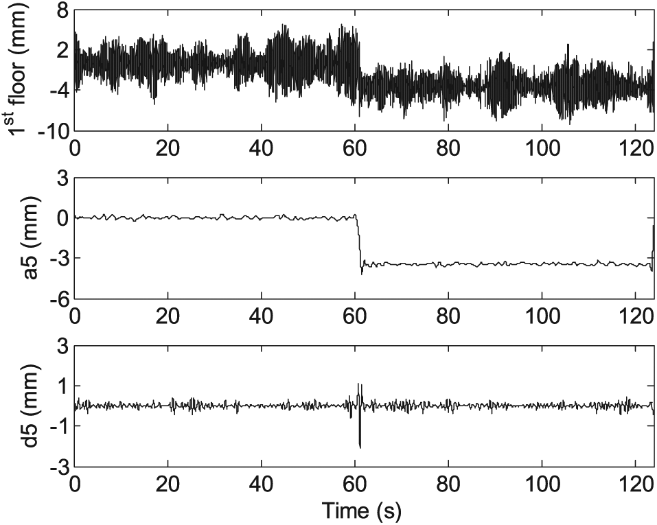
The plot of the displacement of the first floor (the top one), the decomposed scale approximate component of the displacement (the middle one) and the decomposed detail component of the displacement (the bottom one).
The abrupt change time can be determined as 61.18 s from Figure 15. As the same of cases A and B, two proposed methods are applied to the test data in case C, and the identified results are shown in Figure 16.
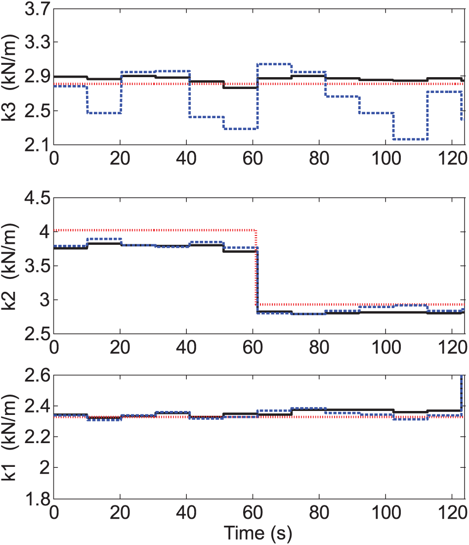
The identified stiffness in case C ( the static tested result, --------the identified result based on DWT, –––the identified result based on substructure and DWT).
For a better comparison of the accuracy between the traditional DWT method with proposed approach, a mean identified error is defined as
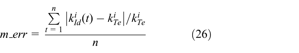
where
The mean identified error of each floor stiffness
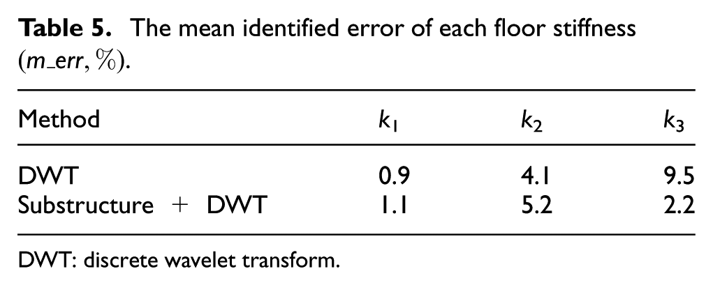
DWT: discrete wavelet transform.
Similarly, the identified result based on DWT has larger fluctuation. When the substructure method is adopted in this case, the stiffness of the first and the third floors can be effectively identified with very small errors. The stiffness of second floor is time-varying, although there is about 5.2% mean error compared with the tested result, and it still can track very well the abrupt changes in the parameter and the whole variation trend. As shown in Table 5, the identified mean error of the first and the second floors using substructure method is slightly larger than that of using DWT method, but for the third floor, the result based on substructure method is far less than that of DWT method. As mentioned previously, there is an overall deviation between practical structure and assumed model, and the uncertainty fluctuation of identified result using the DWT method may somewhat decrease the mean error of the first and second floors, but it greatly increases the error of the third floor.
Conclusion
A DWT and substructure algorithm is presented in this article for tracking the abrupt stiffness degradation of shear structure. Substructural technique can alleviate the ill-posed problem and reduce the dimension of identifying system that will decrease computing consumption for optimizing wavelet parameters and equation solving. There is no need to measure simultaneous the response of all DOFs, which is convenient in application. The use of DWT helps to convert the time-varying parameter identification problem into a time-invariant scale coefficient estimation problem. To obtain the expected identification and to minimize the computational consumption, the criteria based on AIC is adopted to determine the optimal decomposition scale of each time-varying parameter.
Numerical simulation results indicate that the proposed method can effectively identify the time-varying parameter with a satisfactory accuracy. Even if 10% Gaussian white noise is injected to the simulated responses, the method can effectively track the variation of the parameters. The experimental results show that the identified effect combining substructure and DWT is better than that of using only DWT method, and it can be also seen that the “haar” wavelet shows good performance of catching the abrupt variation of structural parameters. The proposed method is suitable for shear-type structural application, which can be used to track not only abrupt variation but also linear changes in the parameter.
This article mainly focused the identification of stiffness, so the mass of model has been tested in advance and updated during identifying procedure. Certainly, when the target structure should be considered as a nonlinear system for damage detection, the mass identification is also an important topic, which is worth doing research in the future.
In addition, the major work in this article is to introduce the substructure method for identifying the time-varying parameter. As a feasibility study, a numerical simulation and a simple model test are used to verify the feasibility and accuracy of the method. Further works such as verification using field test data of a real complex structure, computation efficiency, and accuracy of method are still in progress. Therefore, we will continue this study in the future.
Footnotes
Acknowledgements
The authors thank Professor CG Koh of National University of Singapore for providing constructive suggestions. The authors also thank the reviewers for their suggestions which permit to improve this manuscript.
Declaration of Conflicting Interests
The author(s) declared no potential conflicts of interest with respect to the research, authorship, and/or publication of this article.
Funding
The author(s) disclosed receipt of the following financial support for the research, authorship, and/or publication of this article: This research was supported by the China Scholarship Council (CSC Grant No. 201608420053), the National Natural Science Foundation of China (Grant No. 51408250), PhD Research Startup Foundation of Hubei University of Technology (Grant No. BSQD14043), and the China Postdoctoral Science Foundation (Grant No. 2018M632861).