Influence of elevated water levels on wind field characteristics at a bridge site

Abstract

The influence of elevated water levels on wind field characteristics at bridge sites owing to hydroelectric power stations plays an important role in bridge engineering, particularly in mountainous valley regions. To investigate this issue, a comparative experimental study, which uses a topographic model with two water level states for determining the influence on wind field characteristics at the proposed bridge site located in a mountainous valley area, was conducted in the XNJD-3 wind tunnel at Southwest Jiaotong University, Chengdu, PR China. The altitude difference between the two water level states was approximately 200 m, whereas uniform and D-type boundary layer air inflow conditions were adopted during the wind tunnel test, respectively. The wind speed at the bridge girder and profile of the 1/4, mid, and 3/4 spans were recorded during the experiment. The test results indicated that after the water level was raised, the mean wind speed (or speed-up factor) along the bridge girder decreased by approximately 10%, and the values of the wind profile also decreased. However, the wind profile curve shapes remained approximately unchanged, and the wind attack angle was significantly transformed by approximately 5° in certain locations of the bridge girder. Moreover, the variation in the water level had a negligible influence on the turbulence intensities, turbulence integral length scales, probability distribution of fluctuating wind components, and turbulent wind spectra along the bridge girder. Therefore, as the water level in the canyon rises, the wind field characteristics at the bridge site tend to be conducive to bridge safety. Therefore, long-span bridges located in mountainous valley areas should be designed appropriately according to the expected minimum water level of the river.

Keywords

mean wind mountainous valley topographic test turbulent wind wind characteristics at bridge sites

Introduction

Transportation facilities in the western region have been developed with the rapid development of China’s economy. The long-span bridge, which is one of the important transportation facilities, is extensively designed and constructed in mountain valley terrain of Southwest China, owing to its excellent ability in overcoming large distances. Wind loading has become one of the dominant factors that can cause troubles and even disasters in slender and weak long-span bridges. Meanwhile, current relevant specifications or codes have exposed noticeable deficiencies. For example, the speed-up factors recommended by relevant specifications are often over-predicted for complex terrains (Jubayer and Hangan, 2018; Miller and Davenport, 1998). Therefore, understanding the wind field characteristics of bridge sites located in mountain valley terrains is necessary. Presently, three methods are generally available for investigating the wind field characteristics of a complex terrain, namely, numerical simulation, field measurements, and wind tunnel testing.

Owing to the improvements in computing capabilities, computational fluid dynamics (CFD) is widely employed in the research of complex terrain wind field characteristics (Miller and Davenport, 1998), and the Reynolds averaged Navier Stokes (RANS) and large eddy simulation (LES) methods are extensively applied (Jubayer and Hangan, 2018). The standard k – ε, renormalization group k – ε, standard k – ω, shear stress transport (SST) k – ω, baseline –ω, and Speziale–Sarker–Gatski Reynolds stress model are the most popular turbulence models adopted for simulating the wind flow over complex terrains (Abdi and Bitsuamlak, 2014; Bitsuamlak et al., 2004; Loureiro et al., 2008; Miller and Davenport, 1998). Among these, the SST k – ω turbulent model can provide the most accurate prediction of the mean wind speed and wall shear stress on the windward side. However, the performance on the leeward side is not very effective. The steady-state numerical simulation based on RANS turbulent models only provides steady flow properties but no transient information. Therefore, the LES model has been used to address this issue, but the major challenge in LES is creating appropriate boundary layer inlet conditions with proper turbulence characteristics (Aboshosha et al., 2015; Tabor and Baba-Ahmadi, 2010; Tutar and Celik, 2007). The advantage of the CFD numerical simulation is its low cost, flow field information of any position in the computing domain, and arbitrary calculation area of the terrain and scale. In spite of this advantage, the solution of the leeward side is not very accurate in which numerical simulation cannot replace the field measurements and wind tunnel tests.

Compared with the numerical simulation, field measurements can obtain the most realistic and accurate wind data for in situ wind field characteristics. For example, Busch and Panofsky (1968) and Kaimal et al. (1972) measured the boundary layer wind to obtain the spectra of atmospheric and boundary layer turbulence, respectively. The proposed turbulent wind spectra have been widely adopted in numerous national specifications. Since then, researchers have begun to focus on measuring wind characteristics under special conditions. Shiau (2000) measured the wind characteristics on the northeastern coast of Taiwan under high-wind conditions. Peng et al. (2018) investigated the spatial coherence in near-surface strong winds in Southeast China via field measurements by using several ultrasonic anemometers. Shu et al. (2018) investigated the relationship between the wind direction and height via a Doppler wind profiler and surface weather station in Hong Kong, China. Although field measurements can obtain the most realistic wind characteristics, shortcomings such as high cost, lengthy period, and limited arrangement of the measuring points render it impossible to implement such large-scale activities conveniently.

The disadvantages of both numerical simulation and field measurements can effectively be avoided through wind tunnel tests, and the advantages of wind tunnel tests are of medium cost, shorter period, more accurate test results on the leeward side, and controllable inlet conditions, among others. Miller and Davenport (1998) calculated the speed-up factors of several two-dimensional (2D) complex terrains under two types of incoming wind profiles via a wind tunnel experiment. The results indicated that the speed-up factors predicted by isolated hills or ridges were larger than that of complex terrains. Mattuella et al. (2016) conducted the same types of wind tunnel topographic experiments by using a hot wire anemometer. Particle image velocimetry has also been employed in wind tunnel experiments by several researchers (Lange et al., 2017; Ma et al., 2019b; Rasouli et al., 2009) to obtain wind data for large areas or bridge engineering. However, the cost is higher than that of point measuring tools. Jubayer and Hangan (2018) applied the TFI J-cobra probe to measure the wind velocities at numerous locations on the terrain model. They obtained more realistic results by applying the incoming wind profile calculated from a numerical simulation of a larger terrain domain. Therefore, the wind tunnel test is still extensively used as a reliable method for obtaining wind field parameters. However, the terrain ranges and model sizes in the aforementioned literature are relatively small. Thus, the accuracy of the test results may be affected to certain extent. Consequently, a large terrain model with a diameter of 15 m was employed in the experiment, representing 12 km in the realistic topography.

Although several literatures, specifications, and codes have recommended the wind parameters for mountain valley regions, these were inaccurate and excessively conservative. Given that the influence of elevated water levels on wind field characteristics at bridge sites has rarely been reported, this study fills this gap and augments the research on wind field characteristics in mountain valley areas. Meanwhile, owing to the advantages and disadvantages of numerical simulations and field measurements, respectively, the wind tunnel terrain test is employed to conduct this research. The contents of this article are organized as follows. The section “Topography” describes the topographic features, location of the proposed bridge, and the layout of the measuring points in detail. The “Wind tunnel test model” section discusses some basic information regarding the wind tunnel test models, such as the dimension, scale, material, and model construction process. The sections “XNJD-3 wind tunnel” and “Measurement details” present the information on the XNJD-3 wind tunnel and measuring tool employed, respectively, during the test, incoming flow conditions, and test cases. The section “Results and discussion” discusses the test results of the mean wind characteristics, turbulence statistics. and turbulent spectra with discussions. Finally, the “Concluding remarks” section summarizes several important conclusions of the experimental study.

Topography

The topography investigated herein is the Tiger Leaping Gorge in Diqing Tibetan Autonomous Prefecture, Yunnan Province, China. The topographic map of the Shuttle Radar Topography Mission (STRM) is illustrated in Figure 1, where the red line indicates the proposed bridge. The distance from the proposed bridge girder to the water surface of the Jinsha River is approximately 600 m. During the wind tunnel tests, the wind speed records at a total of 33 locations around the proposed bridge on the terrain. The layout of the 33 measuring points is illustrated in Figure 2. Nine of the 33 measuring points were arranged horizontally and located at the axis of the proposed bridge girder, traversing the topographic valley. The region is located in the Hengduan Mountains in Southwestern China, where the altitude differences are very large. The Tiger Leaping Gorge is formed by the cutting action of the Jinsha River. The mountains on both sides are very high and steep. Particularly, the Haba and Yulong mountains stand on the north and southeast of the valley, respectively. Moreover, the tops of the two mountains are almost covered with snow throughout the year. The elevation of the mountains on the west side of the valley is relatively low. Meanwhile, a tributary flows into the Jinsha River, forming a typical triangular valley. The above topographical features are responsible for the very complex wind field characteristics in the area.

Figure 1.

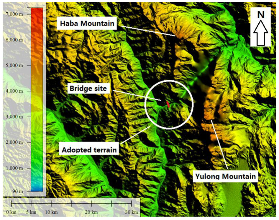
Topography of the bridge site.

Figure 2.

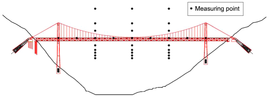
Locations of the measuring points.

The terrain altitude is as same as that of most of the region and ranges from approximately 1630 to 3000 m. The relative elevation difference is approximately 1370 m from the top of mountains to the bottom of the deep valleys. Owing to the significant altitude differences, the Jinsha River, which is a tributary of the Yangtze River, contains over 100 million kilowatts of water resources, accounting for more than 40% of the Yangtze River water resources. Consequently, fully using the advantage of significant hydropower resources is highly suitable for the construction of hydropower stations. For the assumption of the reservoir, the water surface would increase by approximately 200 m, resulting in an evident change in wind field characteristics at the bridge site. The bridge design for wind resistance does not possibly consider the higher water level case after the hydropower station is constructed. Thus, investigating the wind field characteristics via wind tunnel tests for this typical terrain with various water levels is necessary.

Wind tunnel test model

For the wind tunnel test, a 1/800 scale model was established from foam plastic and covered by a green rough layer to reproduce as much local roughness as possible. Two aspects of reasons have been considered for the scale selection. First, the scale of the wind tunnel model should be sufficiently small to reduce the blockage effect of the wind tunnel to ensure the full development of the bridge site wind field. Second, a terrain model scale as large as possible had to be selected for the necessary model precision and interference reduction of the measuring equipment with the airflow (Miller and Davenport, 1998). According to the test model orientation, which only had two directions, namely, upstream inflow condition and downstream inflow condition, the blockage ratio was approximately 19%. Moreover, the two inflow conditions are illustrated in Figure 3. According to Aly et al. (2011), the maximum allowable blockage ratio is 5% for open-jet wind tunnel tests. However, this finding does not mean that the blockage ratio cannot be greater than 5% in all wind tunnel test types, particularly terrain wind tunnel tests. In their study, a 16% blockage ratio based on the jet outlet had less influence on the estimation of the pressure measurements compared with the values reported in the literature. Moreover, according to Jubayer and Hangan (2018), although the largest blockage ratio of approximately 17%, for a specific model orientation based on the contraction outlet area, was measured in the wind tunnel terrain test at the WindEEE dome, no blockage corrections were performed and the results were not significantly affected. Furthermore, as the influence of the change in water level on the wind field characteristics is the subject of this study, the two test models were completely consistent except for the water levels. The test model with higher water level was established by simply filling the river with foam to increase the water level compared with the model with the lower water level. Therefore, even if the influence of the larger blockage ratio is significant, the effect of elevated water level on the results can also be measured and analyzed. Finally, no data correction based on the blockage ratio was implemented in this study.

Figure 3.

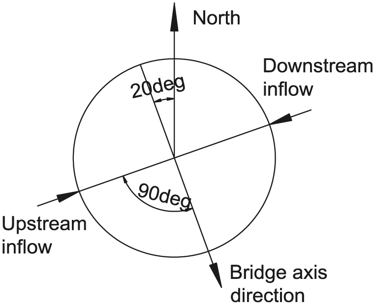
Upstream and downstream inflow conditions.

Owing to the highly complex topographical configuration and lack of a wind model for the deep valley where the proposed bridge is located, the wind tunnel terrain test is a highly suitable and effective method for investigating the wind field characteristics. The wind tunnel test model in this experiment was constructed on the basis of the topographical maps. The test model was mounted on a circular flat with numerous wheels on the bottom for the free rotation around its center. The edge of the terrain model, the center of which coincided with the bridge mid-span, was smoothly cut to ensure that it aligned with the edge of the circular flat. Based on the model-scale ratio of 1/800, the diameter and maximum height of the circular terrain model were 15 and 1.8 m, respectively, corresponding to a realistic terrain with a 12 km diameter and 1.44 km height. Owing to the large scale of the terrain model, the test was performed in the XNJD-3 wind tunnel, which is presently the largest boundary layer wind tunnel in the world, located in the Southwest Jiaotong University, Chengdu, PR China. The terrain model is mounted on the center of the wind tunnel test section, where the width is 22.5 m. Therefore, there are 3.75 m of free space on both sides of the terrain model. Consequently, the effects of the limited capacity of the wind tunnel on the obtained results are negligible.

Although only one terrain model was established, the water level height was increased by approximately 200 m by laying the foam in the river channel. To render the terrain model more realistic, the entire river channel was filled with foam. The terrain models inside the XNJD-3 wind tunnel are illustrated in Figure 4.

Figure 4.

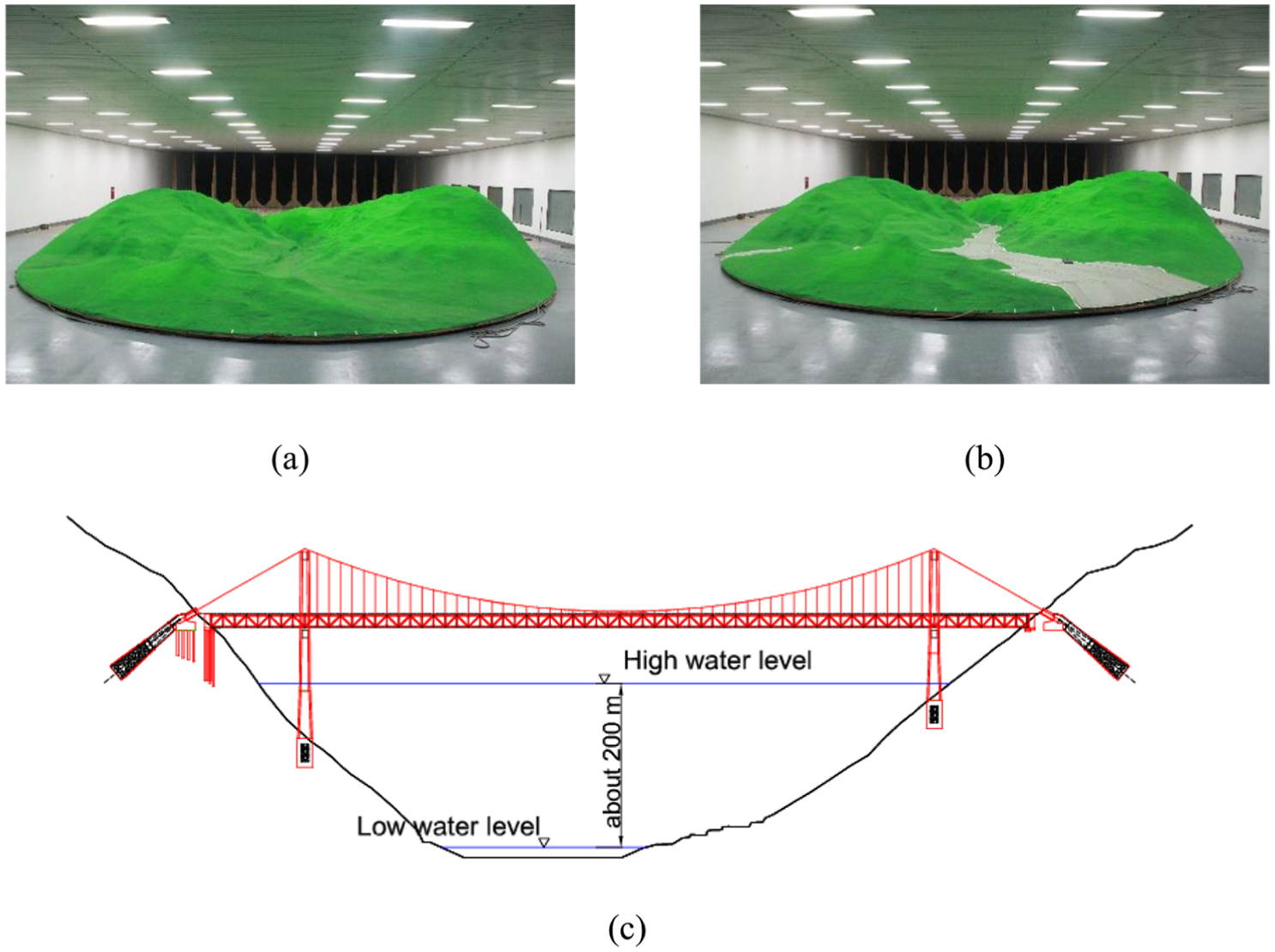
Wind tunnel models in the XNJD-3 wind tunnel: (a) low water level, (b) high water level, and (c) schematic of different water levels.

XNJD-3 wind tunnel

The XNJD-3 wind tunnel at the Research Center for Wind Engineering, Southwest Jiaotong University, Chengdu, PR China, is capable of producing both uniform and several boundary layer inflow conditions matching with the Chinese code (JTG/TD60-01, 2004). The boundary layer inflow conditions were produced using spires and rough elements regularly arranged in the upstream, as illustrated in Figure 4. The wind tunnel test chamber has a rectangular section with a height of 4.5 m and width of 22.5 m, which is ideal for large model tests (Ma et al., 2019a). Four large fans are installed at the front of the test chamber, each with a maximum power of 160 kW. The design wind speed of the wind tunnel is 15 m/s. However, in practice, the maximum wind speed can reach 16.5 m/s when the power of the fans reaches 90%.

In this study, only the uniform and D-type boundary layer inflow conditions in accordance with the Chinese code (JTG/TD60-01, 2004) were employed to conduct the tests. The incoming flow velocity at the bridge girder height was set to 8 m/s to ensure the reliability of the measuring equipment. Owing to its sufficiently large test chamber, the XNJD-3 wind tunnel was selected for the experiment.

Measurement details

A total of 33 locations, as illustrated in Figure 2, were established for measuring the wind speed on the terrain model performed in the XNJD-3 wind tunnel. The wind speeds at different test model locations were measured using the TFI J-cobra probe (Turbulent Flow Instrumentation Pty Ltd.) (Jubayer and Hangan, 2018). The maximum sampling frequency of J-cobra probes can reach up to 2 kHz. The speed range this instrument allows to work is from 2 to 100 m/s, and the measurement accuracy is within ±0.5 m/s (TFI, 2018). During the experiment, the sampling frequency was set to 1.024 kHz for a sampling time of 60 s. Thus, 61,440 data records are present in each measured time series. However, the record data quality was usually 95+%, and the ineffective measurement data were removed during post-processing. The along-wind, and lateral and vertical wind speeds were simultaneously recorded by J-cobra probes to calculate the mean wind speed, pitch angle, and turbulence intensity, among others.

The J-cobra probes were mounted on a door-type shelf, which was placed in an appropriate position on the terrain model. A schematic view of the cobra probes with the door-type shelf is presented in Figure 5. Stick I is fixed on the terrain, whereas stick II can move freely up and down along stick I. Meanwhile, stick III can shift freely left and right along stick II. Sticks I and III are retained in the vertical state, whereas, stick II is parallel to the horizontal plane. The direction of the head of the J-cobra probes is perpendicular to the bridge girder. Moreover, the locations of the J-cobra probes at all the measurement points are strictly verified to ensure measurement accuracy. Meanwhile, the wires are wrapped around the sticks or placed behind the measuring points to ensure the least interference with the measurement of the J-cobra probes. The size of the measuring point of the J-cobra probe is approximately 6.67 mm (5.3 m in a realistic topography).

Figure 5.

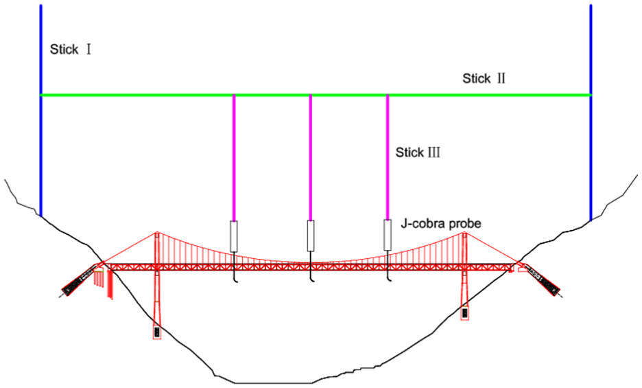
Schematic view of TFI J-cobra probe arrangement.

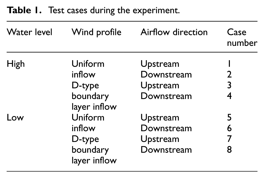
During the experiment, two wind directions were used, namely, upstream and downstream along the river channel, respectively, as well as perpendicular to the proposed bridge. Then, the two incoming wind profiles of uniform and D-type boundary layer inflow conditions, with a power law exponent of 0.3 in accordance with the Chinese Wind-Resistant Design Specification for Highway Bridges (JTG/TD60-01, 2004), were employed during the test. Compared with the uniform inflow condition with constant incoming wind speed, the wind profile matching the D-type boundary layer inflow condition was more realistic based on the complex features of the surrounding topography. The two wind profiles were adopted to produce two extreme wind speed cases at the bridge site in the terrain model. The wind tunnel test cases of this study, according to the water level height of the hydropower station reservoir, wind profile of the inflow condition, and airflow direction are listed in Table 1.

Table 1.

Test cases during the experiment.

Water level	Wind profile	Airflow direction	Case number
High	Uniform inflow	Upstream	1
	Uniform inflow	Downstream	2
	D-type boundary layer inflow	Upstream	3
	D-type boundary layer inflow	Downstream	4
Low	Uniform inflow	Upstream	5
	Uniform inflow	Downstream	6
	D-type boundary layer inflow	Upstream	7
	D-type boundary layer inflow	Downstream	8

Results and discussion

According to the test cases, eight runs of wind raw data were recorded and analyzed, each consisting of wind speed time series of 33 measuring points in the test model. Analytical techniques by using MATLAB® were utilized to obtain the mean wind characteristics, turbulence statistical properties, and turbulent wind spectra.

Mean wind characteristics

The mean wind characteristics, which play an important role in the bridge static wind stability, were processed for eight runs of wind raw data. The results of the mean wind velocity, mean attack angles and wind profiles are illustrated in Figures 6, 7, and 8 to 10, respectively. The ordinate of Figure 6 and abscissa of Figures 8 to 10 represent the mean wind velocity, which is normalized by the incoming flow velocity (V_ref) at the same height as the bridge girder. Particularly, the mean wind velocity in this case is perpendicular to the bridge girder given that the wind speed along the bridge lateral direction receives more attention in the wind-resistant design for bridge engineering. Moreover, the dimensionless mean wind velocity is also known as the speed-up factor as mentioned in numerous literatures.

Figure 6.

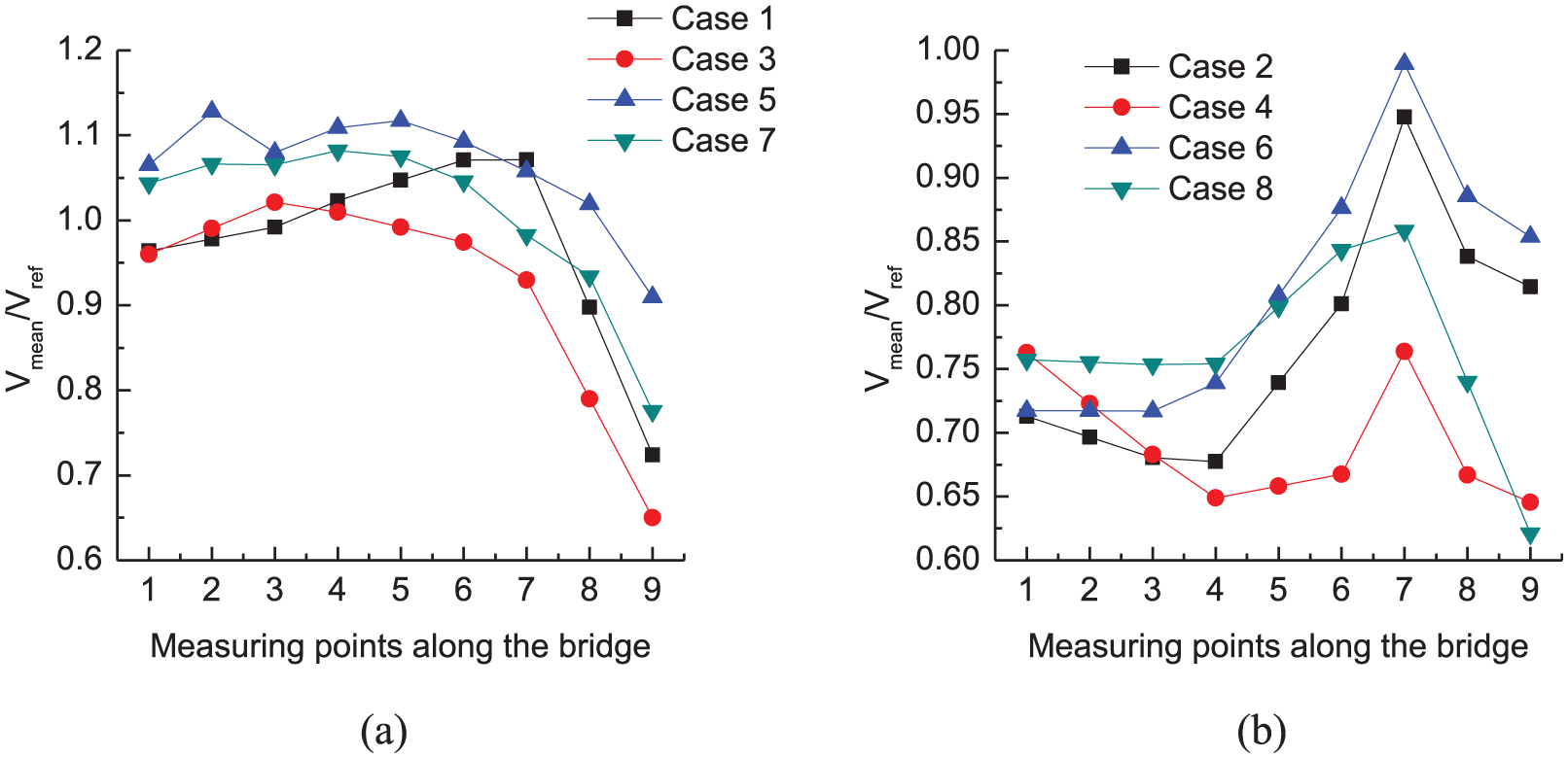
Distribution of normalized mean wind velocity along the bridge girder: (a) upstream and (b) downstream.

Figure 7.

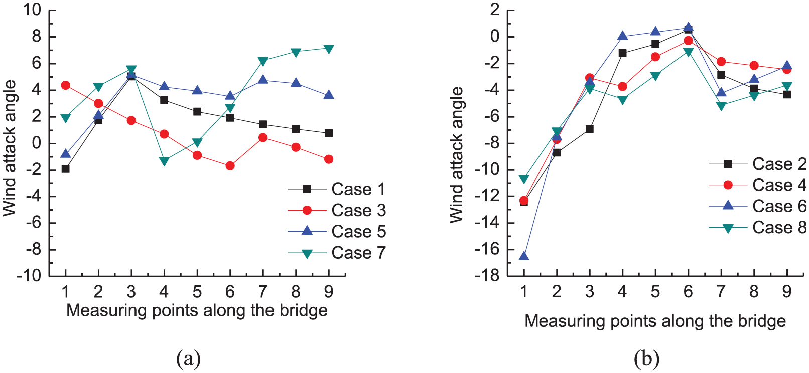
Distribution of the wind attack angle along the bridge girder: (a) upstream and (b) downstream.

Figure 8.

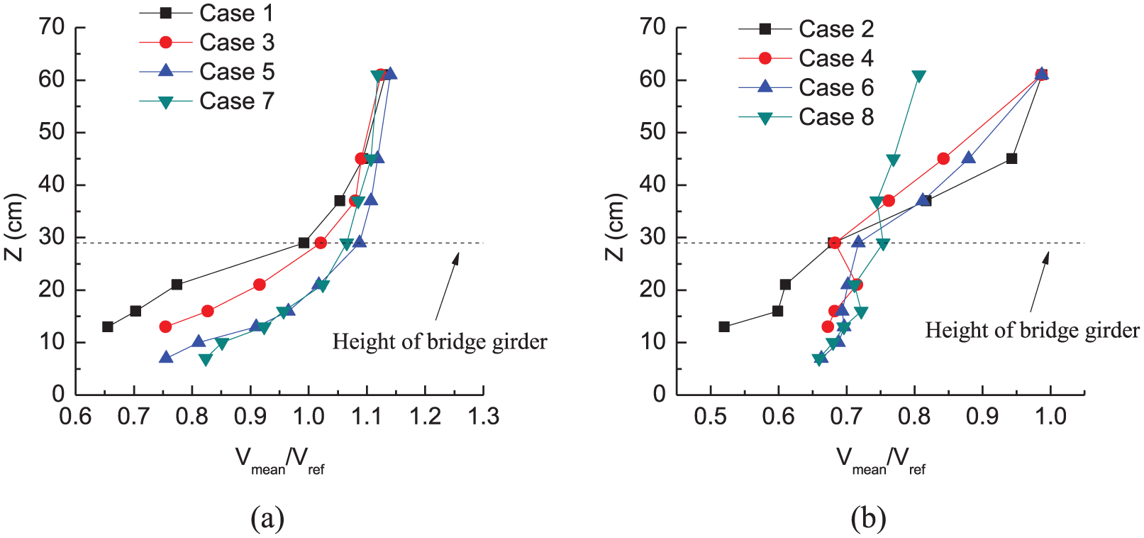
Wind profile at 1/4 span: (a) upstream and (b) downstream.

Figure 9.

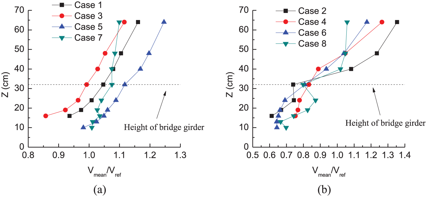
Wind profile at mid-span: (a) upstream and (b) downstream.

Figure 10.

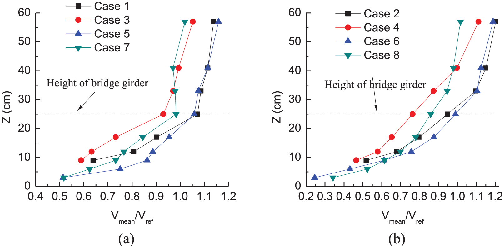
Wind profile at 3/4 span: (a) upstream and (b) downstream.

The normalized mean wind velocity magnitudes of the nine measurement points along the bridge girder, as shown in Figure 2, are plotted in Figure 6 based on the results of the wind tunnel test of the different test cases listed in Table 1. For the sake of convenience, the results are plotted separately according to the incoming flow directions, that is, upstream and downstream. The normalized mean wind velocity at the low water level is generally greater than that at the high water level, but the curve shapes in the figure are basically similar. This finding is owing to the decreasing distance from the bridge girder to the water surface after the water level is raised, and the mean wind velocity proportionally varies with height (as shown in Figures 8 –10) in the boundary layer at this bridge site. Similarly, as shown in each curve of Figure 6(a), the values on the right side are significantly smaller than that on the left side, also owing to the higher altitude of the topography on the right. In this research, after the water level is raised, the mean wind velocity decreases to approximately 90% that of the low water level in both upstream and downstream inflow conditions. The differences in the mean wind velocity between the D-type boundary layer and uniform inflow conditions are relatively small compared with the water level variation. Therefore, the differences in the mean wind velocity caused by the water level require further attention. Moreover, the mean wind velocity obtained from the D-type boundary layer inflow condition is relatively small compared with that obtained from the uniform inflow condition; this finding is in strong agreement with the work of Jubayer and Hangan (Jubayer and Hangan, 2018). Given that the downstream mountains are relatively higher than the upstream ones, the mean wind velocity is relatively small under downstream inflow condition. For example, the maximum mean wind velocities of test cases 5 and 6 are approximately 1.15 and 1.0 for the upstream and downstream inflow conditions, respectively. When the upstream topography is relatively flat, the mean wind velocity along the bridge girder becomes large, regardless of how rugged and steep the bridge site terrain is.

The wind attack angle is also an important argument in bridge wind engineering, thus directly affecting the bridge response with wind loads. Specifically, for the bridge girder section, the force coefficients Cm, Cd, and Cl vary with the wind attack angles. The distributions of the wind attack angles along the bridge girder for the different test cases are illustrated in Figure 7. Evidently, the wind attack angles change significantly with different water levels, particularly for the upstream inflow conditions illustrated in Figure 7(a). There are no noticeable rules identified between the wind attack angles and the water level. Furthermore, the wind attack angles along the proposed bridge girder are greatly affected by the topography surface in the atmospheric boundary layer. For the upstream inflow conditions, the terrain on the windward side of the bridge site changes significantly after the water level is raised, resulting in great variations in the wind attack angles. Meanwhile, the wind attack angles are close to 0° because the windward terrain surface becomes flatter as the water level rises. In contrast, for the downstream inflow conditions, the upstream terrain is so high that the elevated water level has almost no effect on the wind attack angles. Consequently, approximately identical wind attack angles are measured as illustrated in Figure 7(b). Generally, the wind attack angles range from −2° to 8° and from −15° to 0° for the upstream and downstream inflow conditions, respectively.

Figures 8 to 10 illustrate the wind profiles at the 1/4, mid, and 3/4 spans, respectively. The raised water level has a significant influence on the wind profile compared with the inflow conditions. The value of the wind profiles is relatively small at the same height for high water levels because the distance from the water surface to the bridge girder is reduced, particularly when the surface on the windward side is flat. Generally, the logarithmic and power laws have been used to describe the wind profiles in the atmospheric boundary layers (Davenport, 1960; Davies et al., 2004; Kikumoto et al., 2017). From the results illustrated in Figures 8 to 10, when the upstream topography is flat and low, the logarithmic or power laws can express the wind profiles effectively with appropriate parameters. Nevertheless, the above two types of wind profile models are no longer applicable for rugged and high upstream topography. Consequently, applying the two aforementioned wind profile models, which are usually outlined in the relevant specifications, is not appropriate to simulate rugged and complicated situations. However, although the wind speeds decrease in the high water level cases, the wind profile shapes hardly change, thereby indicating that the terrain roughness factor is almost unaffected after the water level is raised.

Turbulence statistical properties

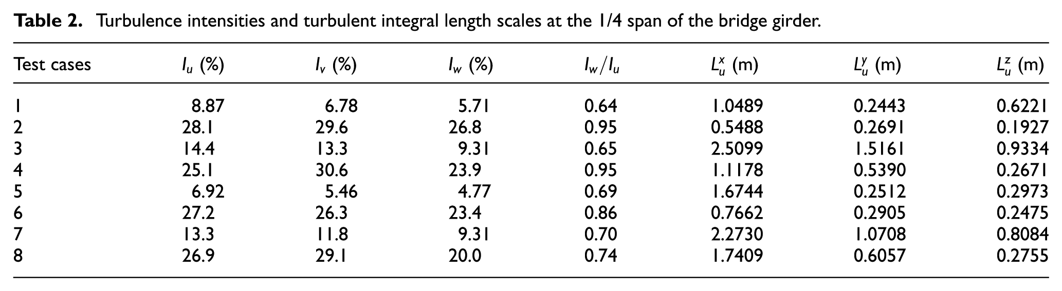
To explain the problem briefly and focus on bridge girder, eight runs of wind records for the three measuring points (i.e. 1/4, mid, and 3/4 spans) are processed to obtain the turbulent wind parameters, the results of which are listed in Tables 2 to 4. The tables also present the turbulence intensity and the longitudinal turbulent integral length scales for the longitudinal, lateral, and vertical direction turbulence ( $L_{u}^{x}, L_{u}^{y}, L_{u}^{z}$ ), respectively. Notably, the directions of the three turbulent wind velocity components, which are determined by the direction of the mean wind velocity during the sampling period of 60 s, differ from that in section “Mean wind characteristics.”

Table 2.

Turbulence intensities and turbulent integral length scales at the 1/4 span of the bridge girder.

Test cases	$I_{u}$ (%)	$I_{v}$ (%)	$I_{w}$ (%)	$I_{w} / I_{u}$	$L_{u}^{x}$ (m)	$L_{u}^{y}$ (m)	$L_{u}^{z}$ (m)
1	8.87	6.78	5.71	0.64	1.0489	0.2443	0.6221
2	28.1	29.6	26.8	0.95	0.5488	0.2691	0.1927
3	14.4	13.3	9.31	0.65	2.5099	1.5161	0.9334
4	25.1	30.6	23.9	0.95	1.1178	0.5390	0.2671
5	6.92	5.46	4.77	0.69	1.6744	0.2512	0.2973
6	27.2	26.3	23.4	0.86	0.7662	0.2905	0.2475
7	13.3	11.8	9.31	0.70	2.2730	1.0708	0.8084
8	26.9	29.1	20.0	0.74	1.7409	0.6057	0.2755

Table 3.

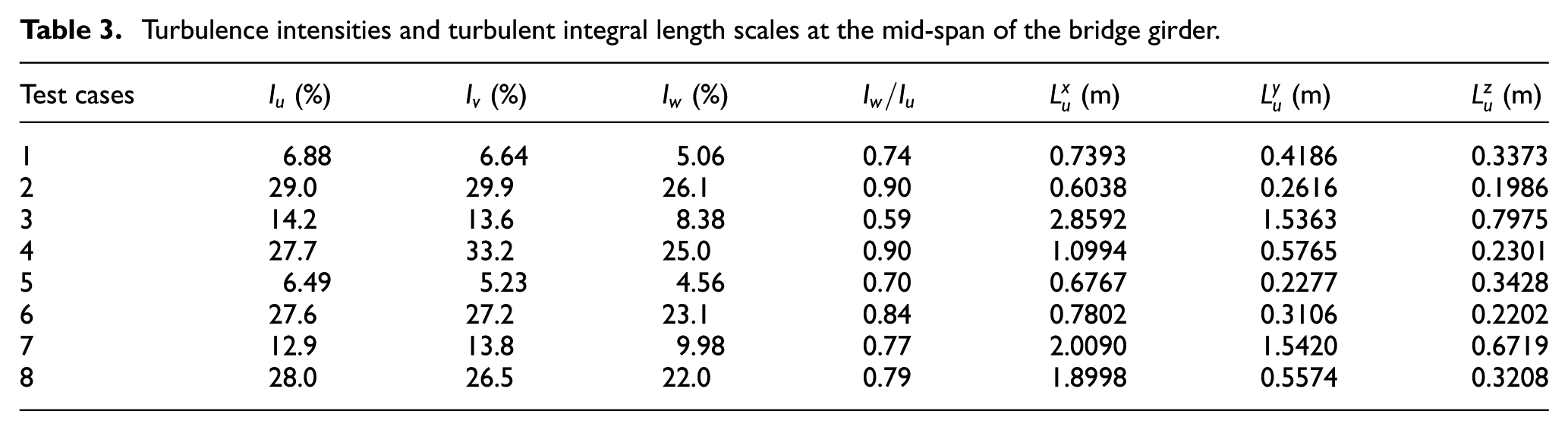
Turbulence intensities and turbulent integral length scales at the mid-span of the bridge girder.

Test cases	$I_{u}$ (%)	$I_{v}$ (%)	$I_{w}$ (%)	$I_{w} / I_{u}$	$L_{u}^{x}$ (m)	$L_{u}^{y}$ (m)	$L_{u}^{z}$ (m)
1	6.88	6.64	5.06	0.74	0.7393	0.4186	0.3373
2	29.0	29.9	26.1	0.90	0.6038	0.2616	0.1986
3	14.2	13.6	8.38	0.59	2.8592	1.5363	0.7975
4	27.7	33.2	25.0	0.90	1.0994	0.5765	0.2301
5	6.49	5.23	4.56	0.70	0.6767	0.2277	0.3428
6	27.6	27.2	23.1	0.84	0.7802	0.3106	0.2202
7	12.9	13.8	9.98	0.77	2.0090	1.5420	0.6719
8	28.0	26.5	22.0	0.79	1.8998	0.5574	0.3208

Table 4.

Turbulence intensities and turbulent integral length scales at the 3/4 span of the bridge girder.

Test cases	$I_{u}$ (%)	$I_{v}$ (%)	$I_{w}$ (%)	$I_{w} / I_{u}$	$L_{u}^{x}$ (m)	$L_{u}^{y}$ (m)	$L_{u}^{z}$ (m)
1	8.38	8.27	5.45	0.65	0.6480	0.5390	0.3512
2	28.1	22.9	20.3	0.72	0.9353	0.2702	0.2233
3	20.0	17.1	11.9	0.60	2.5812	1.7759	0.4736
4	35.4	28.3	24.2	0.68	1.6790	0.4147	0.2985
5	7.38	6.43	5.40	0.73	0.6213	0.3306	0.2422
6	25.0	21.4	19.6	0.78	0.9056	0.3107	0.2805
7	14.0	14.5	11.0	0.79	1.6800	2.2334	0.6436
8	25.9	21.6	18.5	0.71	1.2564	0.4169	0.3420

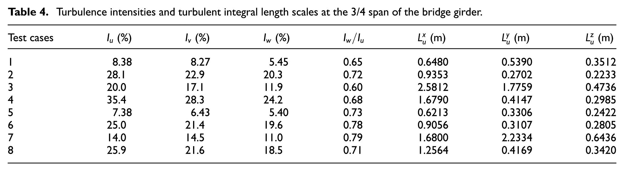
The turbulence intensity is defined as the ratio of the standard deviation and mean wind velocity, representing the fluctuating wind velocity intensity. The test results of the turbulence intensity are listed in Tables 2 to 4. Evidently, the influence of the elevated water level on the turbulence intensity is relatively small compared with that of the inflow conditions or upstream high terrains. Moreover, the turbulence intensities increase slightly as the water level is raised. The reason is that the distance from the bridge girder to the ground surface is reduced, and the flow field is greatly disturbed by the ground. Generally, a smaller distance results in a greater turbulence intensity. Furthermore, the inflow conditions and upstream terrain play a very large role in the turbulence intensities of the bridge girder, and the difference in turbulence intensities is very large. For example, the maximum of $I_{u}$ at the 3/4 span of the bridge girder among the eight test cases is 35.4%, and the corresponding minimum value is only 7.38%, which is 1/5 of the maximum. Furthermore, in Tables 2 to 4, the ratios $I_{w}$ and $I_{u}$ of the high water level are often larger than that of the low water level, except in certain cases. This result indicated that the elevated water level will relatively increase the interference with the wind speed vertical component. The ratios are typically large when the proposed bridge is on the leeward side, owing to the disturbance of the mountains, and vice versa.

The turbulent integral length scale represents the mean vortex scale of the fluctuating wind (Peng et al., 2018), which can be calculated using equation (1) (Bai et al., 2012; Lothon et al., 2006) based on Taylor’s hypothesis

L_{u}^{x} = \frac{\bar{U}}{σ_{u}^{2}} \int_{0}^{\infty} R_{u} (τ) d τ

(1)

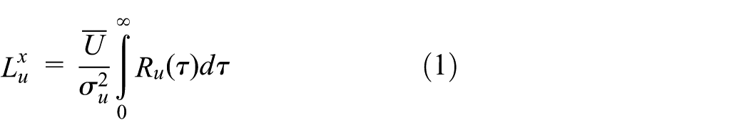
where $\bar{U}$ denotes the mean wind velocity at the measuring point, $σ_{u}^{2}$ is the variance of the fluctuating wind velocity, and $R_{u} (τ)$ indicates the autocorrelation function of the fluctuating wind velocity of $u (x, t + τ)$ and $R_{u} (0) = σ_{u}^{2}$ . Flay and Stevenson (1998) suggested using $R_{u} (τ) = 0.05 σ_{u}^{2}$ as the upper limit of the integral equation.

The turbulent integral length scales at the 1/4, mid, and 3/4 spans of the bridge girder are also calculated using equation (1) and are listed in Tables 2 to 4. As presented in the tables, the turbulent integral length scales exhibit the same trend as the turbulence intensities for different water levels. Moreover, the inflow conditions and upstream terrains have a larger influence than the water level on the turbulent integral length scale. When the proposed bridge is located on the leeward side, the turbulent integral length scale is often very large, and vice versa. This finding indicated that large-scale vortices will be generated by upstream high and steep terrain owing to the adverse pressure gradient and large flow separation. The maximum turbulent integral length scale is approximately five times as large as the minimum. However, the turbulent integral length scale is minimally affected by the changes in the water level.

Figure 11 illustrates the probability density functions (PDFs) of three turbulent components for test cases 1 and 5 at the 1/4 span under the upstream inflow condition. As shown in the figure, the distributions are in strong agreement with the Gaussian distributions. Almost all cases of the measurement data at the bridge girder indicate similar properties, which do not change substantially by raising the water level, although a slight change in size is evident. As also shown in the figure, the turbulent wind speed is more concentrated after the water level is raised, and the variance of the PDFs becomes smaller. The reason of this phenomenon is that the upstream terrain became flatter after the water level is raised, possibly causing less interference with the fluctuating wind speed, although the distance from the surface to the bridge girder is decreased.

Figure 11.

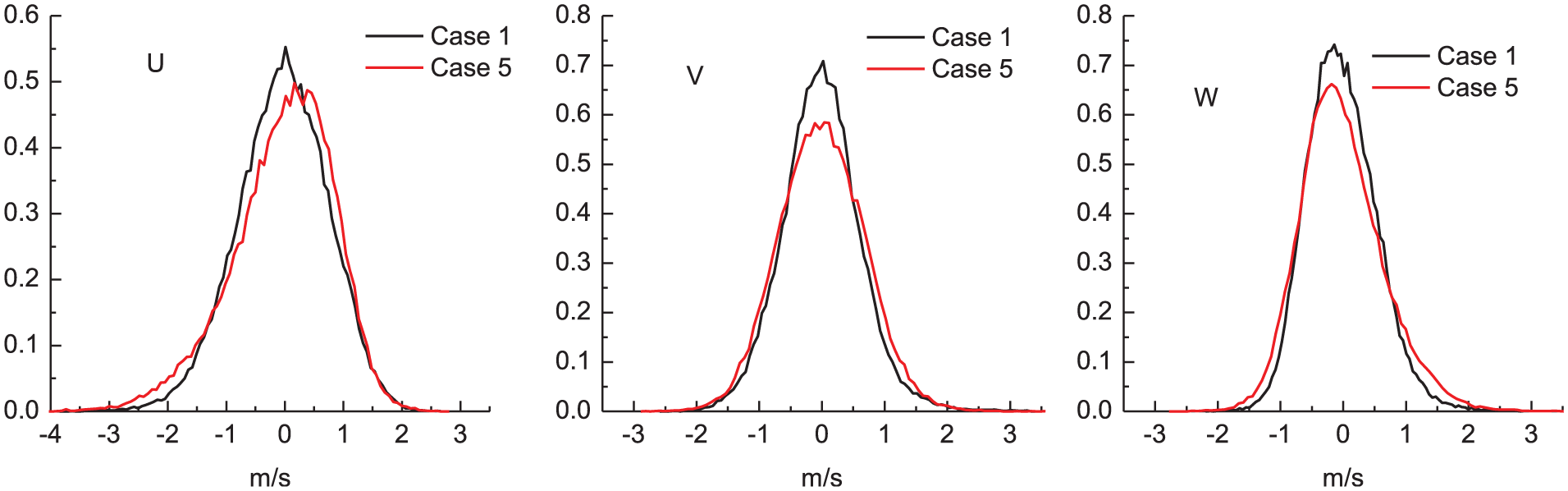
PDFs for three turbulent velocity components, respectively (cases 1 and 5, 1/4 span).

Turbulent wind spectra

The power spectral density function represents the contribution of every frequency component of the turbulent wind velocity in the frequency domain. To obtain smooth power spectral curves, the wind record data of test cases 1 and 5 at the 1/4 span of the bridge girder are processed via the pyulear function in MATLAB to estimate the power spectral density function of the three turbulent wind components, namely, u, v, and w, respectively. The order of the pyulear function, which is determined by the minimum prediction error power of the model, is set to 15. The minimum prediction error power of the model monotonically decreases with increasing order. When the order is taken as 15, the change in prediction error power is almost negligible. First, the spectra of the 1/4 span for test case 1 are calculated to exhibit the differences among the longitudinal, lateral, and vertical components. For the sake of comparison, the results are illustrated in Figure 12 in which the ordinate is the estimated power spectral density normalized by the variances of the three turbulent wind components, respectively. As shown in the figure, the dimensionless power spectral density of the longitudinal components is larger than that of the lateral or vertical components in the low-frequency domain. However, it decreases in the high-frequency domain. Moreover, the slope of the dimensionless power spectral density for the three turbulent wind components is almost −5/3 in the high-frequency domain, which is also known as the inertial spectrum sub-range. The test results of the −5/3 distribution of wind PSD in the sub-range, to a certain extent, demonstrated that the adopted order of 15 was correct and the wind tunnel test data were reliable. The value of −5/3 was also obtained by Kaimal et al. (1972) in the atmospheric boundary layer. The result indicated that the wind field power spectrum at the bridge site in the complex mountain area also agrees with the general power spectra law reported in previous literatures.

Figure 12.

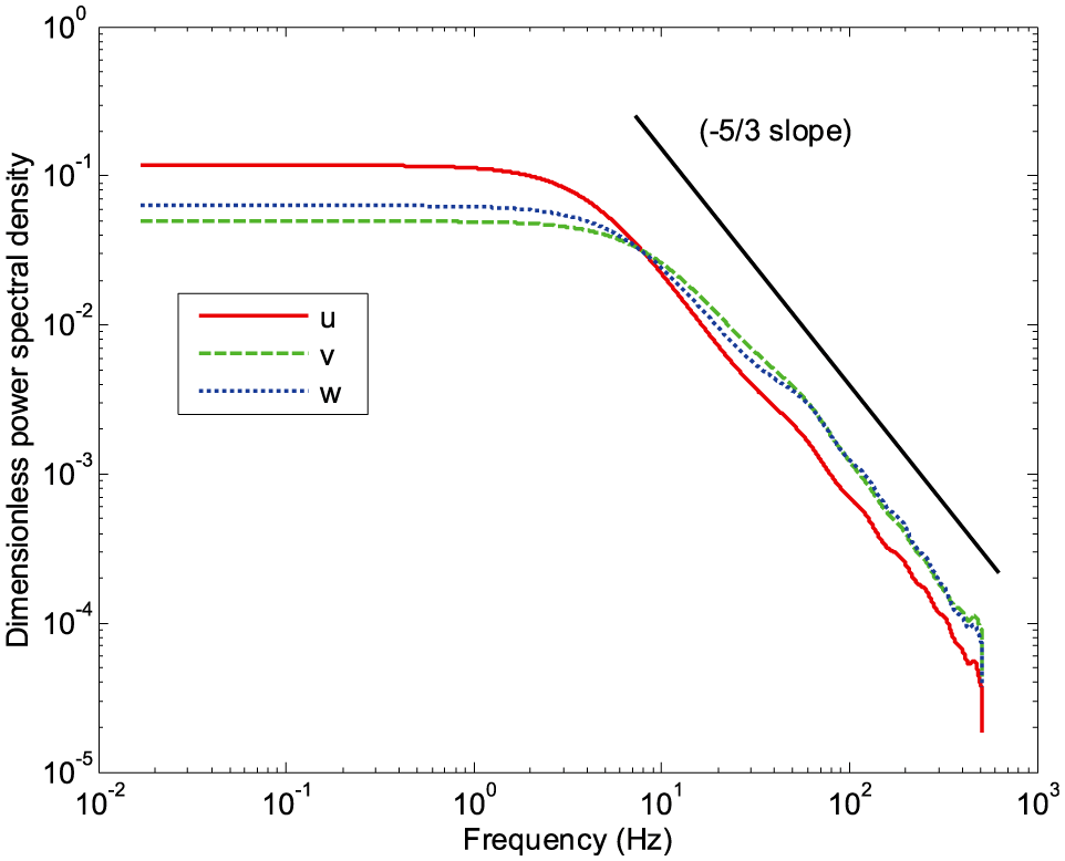
Turbulent wind velocity power spectra of longitudinal, lateral, and vertical components at the 1/4 span for test case 1.

The dimensionless power spectral densities of the three turbulent wind velocities at the 1/4 span for test cases 1 and 5 are illustrated in Figure 13. As shown in the figure, the dimensionless power spectral density of the vertical (w) component is more critically affected than that of the other two components (u and v) after the water level is raised. For the longitudinal (u) component, the dimensionless power spectral density decreases slightly after the water level is raised. Meanwhile, that of the lateral and vertical components (u and v) increase in the low-frequency domain and decrease in the high-frequency domain. This result is possibly because the upstream terrain becomes flatter after the water level is raised, which would reduce the wind fluctuations. However, the power spectral density is almost unaffected by the water level changes, although the water level is raised by approximately 200 m. The results of the other cases exhibit the same phenomenon. Hence, the tests are not repeated.

Figure 13.

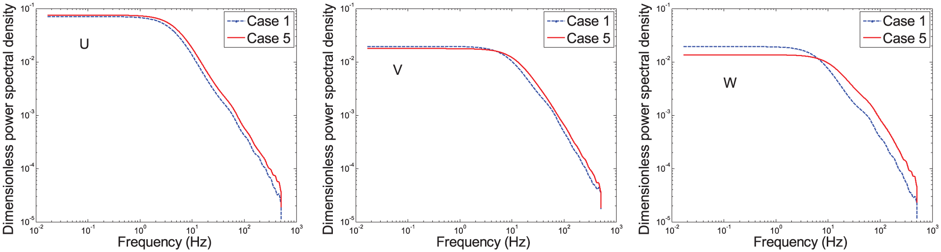
Turbulent wind velocity power spectra of longitudinal, lateral, and vertical components at the 1/4 span for test cases 1 and 5, respectively.

Concluding remarks

A comparative experimental study, which uses a terrain model with two states of water level for determining the influence on wind field characteristics at a bridge site located in the Tiger Leaping Gorge, was conducted in the XNJD-3 wind tunnel at Southwest Jiaotong University, Chengdu, PR China. Low and high water levels, with a difference of approximately 200 m, were the two terrain model states adopted in the wind tunnel test. Meanwhile, the uniform and D-type boundary layer inflow were the two inlet conditions applied during the experiment. The results of the wind tunnel test were processed to analyze the mean wind characteristics, turbulence statistical properties, and turbulent wind spectra. The major concluding remarks can be summarized as follows:

The mean wind velocity at low water level is generally greater than that at high water level. However, the curve shape of the mean wind velocity along the bridge girder is consistent. After the water level rises, the mean wind velocity decreases to approximately 90% of the low water level for both the upstream and downstream inflow conditions. The difference in the mean wind velocity caused by the D-type boundary layer and uniform inflow conditions are relatively small compared with the variation based on the water level. The wind attack angles range from approximately −2° to 8° and from −15° to 0° for the upstream and downstream inflow conditions, respectively. Moreover, these angles change significantly with the different water levels and no noticeable rules are identified. The wind profile values are relatively small at the same height for the high water level, and the wind profile curve shapes hardly change.

The turbulence intensities increase slightly after the water level rises. The turbulent integral length scales exhibit a similar trend to the turbulence intensities for different water levels. The distributions of the PDFs of the three turbulent components exhibit an agreement with the Gaussian distributions. Meanwhile, the turbulent wind speed becomes more concentrated after the water level is raised, and the variance of the PDFs becomes smaller.

The slope of the dimensionless power spectral density for the three turbulent wind components is almost −5/3 in the inertial spectrum sub-range. This result agrees with the general power spectra law in the atmospheric boundary layer. Only minor discrepancies exist in the values. For the longitudinal component, the dimensionless power spectral density decreases slightly after the water level is raised. Meanwhile, the values for the lateral and vertical components increase in the low-frequency domain and decrease in the high-frequency domain. However, the power spectral density is almost unaffected by the water level changes, although the water level is raised by approximately 200 m.

Finally, when the water level is raised, the mean wind velocities and the mean wind attack angles should be paid more attention to prevent damage for the long-span bridges. However, the long-span bridges located on mountainous valley areas should be appropriately designed according to the expected minimum water level, which is the most unfavorable for bridge safety. Moreover, for the complex terrains and atmospheric wind environment, the wind field characteristics at the bridge site are not only affected by water level height, but also by numerous factors. More researches about wind field characteristics on the water level or other factors should be conducted in the next work.

Footnotes

Declaration of Conflicting Interests

The author(s) declared no potential conflicts of interest with respect to the research, authorship, and/or publication of this article.

Funding

The author(s) disclosed receipt of the following financial support for the research, authorship, and/or publication of this article: The work described in this article was fully supported by the National Natural Science Foundation of China (No. 51778545).

ORCID iD

Cunming Ma

References

Abdi

Bitsuamlak

(2014) Wind flow simulations on idealized and real complex terrain using various turbulence models. Advances in Engineering Software 75: 30–41.

Aboshosha

Elshaer

Bitsuamlak

et al . (2015) Consistent inflow turbulence generator for LES evaluation of wind-induced responses for tall buildings. Journal of Wind Engineering and Industrial Aerodynamics 142: 198–216.

Aly

Chowdhury

Bitsuamlak

(2011) Wind profile management and blockage assessment for a new 12-fan Wall of Wind facility at FIU. Wind and Structure 14: 285–300.

Bai

Liu

(2012) Experimental study on wind field characteristics of Sanshui river bridge site located in west valley region. Journal of Vibration and Shock 31: 74–78.

Bitsuamlak

Stathopoulos

Bedard

(2004) Numerical evaluation of wind flow over complex terrain: review. Journal of Aerospace Engineering 17: 135–145.

Busch

Panofsky

(1968) Recent spectra of atmospheric turbulence. Quarterly Journal of the Royal Meteorological Society 94: 132–148.

Davenport

(1960) Rationale for determining design wind velocities. Journal of the Structural Division 86: 39–68.

Davies

Collier

Pearson

et al . (2004) Doppler Lidar measurements of turbulent structure function over an urban area. Journal of Atmospheric and Oceanic Technology 21: 753–761.

Flay

RGJ

Stevenson

(1998) Integral length scales in strong winds below 20 m. Journal of Wind Engineering and Industrial Aerodynamics 28: 21–30.

10.

JTG/TD60-01 (2004) Wind-resistant design specification for highway bridges.

11.

Jubayer

Hangan

(2018) A hybrid approach for evaluating wind flow over a complex terrain. Journal of Wind Engineering and Industrial Aerodynamics 175: 65–76.

12.

Kaimal

Wyngaard

Izumi

et al . (1972) Spectral characteristics of surface layer turbulence. Quarterly Journal of the Royal Meteorological Society 98: 563–589.

13.

Kikumoto

Ooka

Sugawara

et al . (2017) Observational study of power-law approximation of wind profiles within an urban boundary layer for various wind conditions. Journal of Wind Engineering and Industrial Aerodynamics 164: 13–21.

14.

Lange

Mann

Berg

et al . (2017) For wind turbines in complex terrain, the devil is in the detail. Environmental Research Letters 12: 1–8.

15.

Lothon

Lenschow

Mayor

(2006) Coherence and scale of vertical velocity in the convective boundary layer from a Doppler LIDAR. Boundary-Layer Meteorology 121: 521–536.

16.

Loureiro

JBR

Alho

ATP

Silva Freire

(2008) The numerical computation of near-wall turbulent flow over a steep hill. Journal of Wind Engineering and Industrial Aerodynamics 96: 540–561.

17.

Yang

Ngai

et al . (2019a) Experimental study of across-wind aerodynamic behavior of a bridge tower. Journal of Bridge Engineering 24(2): 04018116.

18.

Wang

et al . (2019b) 3D aerodynamic admittances of streamlined box bridge decks. Engineering Structures 179: 321-331.

19.

Mattuella

JML

Loredo-Souza

Oliveira

MGK

et al . (2016) Wind tunnel experimental analysis of a complex terrain micrositing. Renewable and Sustainable Energy Reviews 54: 110–119.

20.

Miller

Davenport

(1998) Guidelines for the calculation of wind speed-ups in complex terrain. Journal of Wind Engineering and Industrial Aerodynamics 74–76: 189–197.

21.

Peng

Wang

(2018) Field measurement and investigation of spatial coherence for near-surface strong winds in Southeast China. Journal of Wind Engineering and Industrial Aerodynamics 172: 423–440.

22.

Rasouli

Hangan

Siddiqui

(2009) PIV measurements for a complex topographic terrain. Journal of Wind Engineering and Industrial Aerodynamics 97: 242–254.

23.

Shiau

(2000) Velocity spectra and turbulence statistics at the northeastern coast of Taiwan under high-wind conditions. Journal of Wind Engineering and Industrial Aerodynamics 88: 139–151.

24.

Shu

et al . (2018) Observational study of veering wind by Doppler wind profiler and surface weather station. Journal of Wind Engineering and Industrial Aerodynamics 178: 18–25.

25.

Tabor

Baba-Ahmadi

(2010) Inlet conditions for large eddy simulation: a review. Computer and Fluid 39: 553–567.

26.

TFI (2018) Cobra Probe. Available at: https://www.turbulentflow.com.au/Products/CobraProbe/CobraProbe.php

27.

Tutar

Celik

(2007) Large eddy simulation of a square cylinder flow: modelling of inflow turbulence. Wind and Structure 10: 511–532.