
Abstract
The load–response correlation method has been recognized by the wind engineering community as a useful equivalent static wind load calculation method for structural design of quasi-static structures against strong winds. However, it has been found that the load–response correlation method is less effective to non-linear systems and in situations where load processes are non-Gaussian, such as large cooling towers subjected to strong winds. To validate the applicability of the load–response correlation method to large cooling towers, an aero-elastic model has been designed for a 215-m-high cooling tower in this article, which can simultaneously produce wind loads and wind-induced displacements of the structure according to wind tunnel model tests. Using data measured on the aero-elastic model, the exact results of correlation coefficients between wind loads and structural responses are obtained and validated by a non-linear finite element analysis. By comparing the correlation coefficients measured on the scaled model to the results based on the load–response correlation calculation, it is found that the correlations are much stronger for the load–response correlation calculation than those for the exact wind tunnel measurement. The explanation for this observation is that the non-linearity of the real structure and the non-Gaussian feature of the actual wind loads can weaken the correlations between the wind loads and the structural responses.
Keywords
Introduction
Guided by Codes of Practice, the gust response factor (GRF) method proposed by Davenport (1967) has been widely used to calculate the equivalent static wind loads (ESWLs) for structural design in many countries. However, as pointed out by Kasperski and Niemann (1992), some deficiencies exist for the GRF: (1) the GRF method will not lead to a result if the mean of either the load or the response is zero; (2) for more than one response to be considered for the design, the GRF method requires further comments concerning the problem of which load is to be used for which response; and (3) the equivalent static load defined using the GRF method may lead to load distributions which lie outside the physical boundaries of local pressures. To this end, the load–response correlation (LRC) method is proposed by Kasperski (1992) for quasi-static structures. Based on correlation analysis, the LRC method addresses the deficiencies with the GRF method (Kasperski and Niemann, 1992) and can produce actual extreme load patterns (Tamura et al., 2002). For a more economical design, the LRC method could be attempted for quasi-static structures, for example, large cooling towers (Niemann, 1980).
However, it must be recognized that the LRC method also has its limitations in use (Kasperski, 1992): (1) an extension of this method to non-linear systems will turn out to be less effective, since non-linear effects will reduce the LRC; (2) the method will be less effective in situations where load processes are not Gaussian, especially when the non-Gaussian properties of the loads are well correlated. Unfortunately, large cooling towers are found to be of material non-linearity (Gupta and Maestrini, 1986; Hara et al., 1994; Waszczyszyn et al., 2000) and geometrical non-linearity (Gao et al., 2001; Waszczyszyn et al., 2000). Besides, non-Gaussian wind pressure fluctuations are observed by Ke and Ge (2015) in side regions on the tower shell, which are likely to be caused by organized large-scale vortexes. To this end, applications of the LRC method to structural designs of large cooling towers should be justified for their rationality, a topic which the article is focused on.
In this article, an aero-elastic model is designed for a 215-m-high large cooling tower, which can truthfully reflect the structure’s non-linearity and the non-Gaussian properties of wind loads on the structure. The wind-induced pressures and structural responses are simultaneously measured on the aero-elastic model in a wind tunnel. Both experimental data are utilized to validate the applicability of the LRC method in approximating the realistic extreme load pattern on large cooling towers.
Wind tunnel model test
Engineering background
Engineering background is a 215-m-high large cooling tower located in a four-tower group with linear arrangement (see Figure 1), which are currently under construction in China. It will be the largest cooling tower in the world with respect to the tower height and the drenching area.

Bird view of the tower group of linear arrangement.
To obtain its dynamic properties, the cooling tower has been simulated on a commercial finite element (FE) platform. The main body is discretized into shell elements, and the herringbone columns are modeled by beam elements. The calculated results listed in Table 1 suggest that the structure’s fundamental modal frequency is 0.658 Hz; the 1–10 lowest order modal frequencies are no greater than 1 Hz; and the mode shapes feature complicated harmonic waves in both circumferential and meridian directions. Since the energy of wind excitations typically accumulates in the frequency range 0.01–0.1 Hz, strong resonances cannot be easily excited by winds for the large cooling tower, the fundamental frequency of which is greater than 0.6 Hz. Thus, the large cooling tower is basically a quasi-static structure and the LRC method can be applied in this regard.
Calculated natural frequencies and mode shapes according to FE analysis.
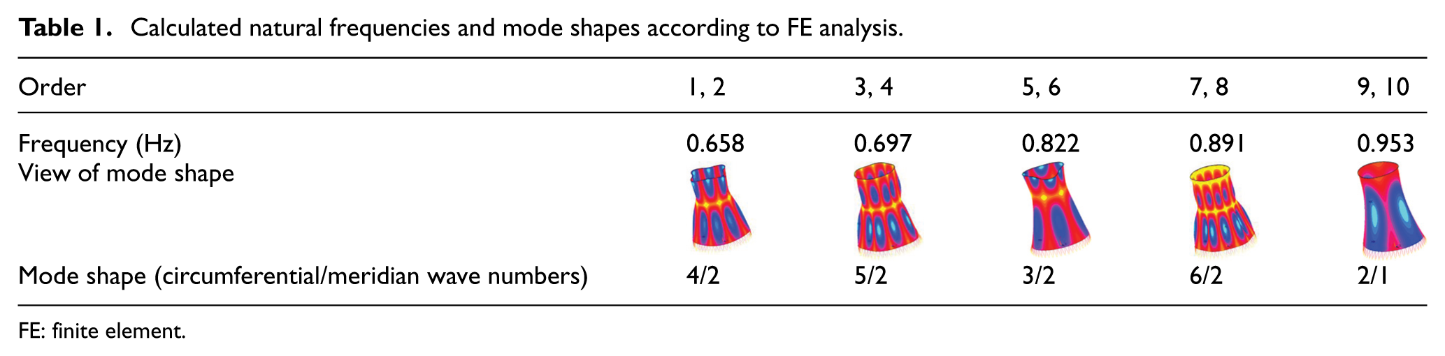
FE: finite element.
Aero-elastic model design
The traditional aero-elastic models for cooling towers are manufactured using continuous medium shell material, which have the shortage of the likelihood of physical parameters. Since the targeted scaling ratio of elastic modulus and shear modulus cannot be truthfully simulated due to the limitation of material selection, the thickness of the isotropic continuous medium thin shell must be adjusted to satisfy the scaling requirement of the bending/torsion stiffness of the thin wall. However, when the scaling requirement of the bending/torsion stiffness is satisfied, the simulated axial stiffness is usually much greater than the targeted value due to the difference of the two to three orders of magnitude between the axial stiffness and the bending/torsion stiffness of the thin wall. The results of approximate simulation will inevitably cause the mismatch of the model’s dynamic characteristics and the design requirements.
To this end, an innovative beam-net aero-elastic model is proposed for cooling tower model tests, with the main purpose of truthfully simulating the large shell’s dynamic characteristics by means of a spatial truss structure. For any local position on the beam-net model, both the thickness and the width of the orthogonal truss unit can be adjusted, so that different types of stiffness scaling can be simultaneously realized on the aero-elastic model. The main steps in manufacturing a beam-net aero-elastic model are as follows:
Step 1. Use FE calculation to obtain the cooling tower’s dynamic characteristics from a detailed numerical model.
Step 2. Establish a numerical model for the beam-net aero-elastic model, wherein the number of meridian beam elements is m and the number of circular beam elements is n; considering the circular symmetry of the cooling tower, the meridian thickness and width variables can be simplified to
Step 3. For a convenient processing of the model, use continuous components with equal thickness as the meridian beam element. Thus,
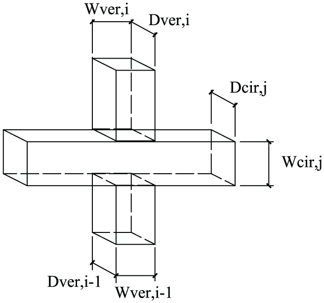
Geometrical sizes of a node on the aero-elastic model.
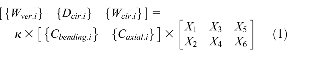
Since a large number of nodes are connected by welding, the cumulative effect of stiffness loss in the node is large. Thus, a stiffness commutation factor κ is introduced in equation (1). In equation (1), the number of variables is simplified to 6–7 (X1 to X6). Generally, 6–8 low-order modes calculated using the detailed numerical model can be regarded as the simulation targets. The initial values X1 to X6 should be provided. Then, through iterative optimization on the beam-net numerical model, the correct values of X1 to X6 can be obtained when the beam-net numerical model’s low-order modes agree with those of the detailed numerical model.
Overview of the model test
Model tests were undertaken in a TJ-3 atmospheric boundary layer (ABL) wind tunnel in Tongji University, China, a closed-circuit rectangular cross-section wind tunnel. The dimensions of the test section were 15 m wide, 2 m high, and 14 m long. As per GB/T 50102-2003 (2003), a Type B ABL turbulent flow field was simulated for the model tests using the conventional spire–roughness passive simulation method. The characteristics for the simulated flow field were measured using a hotline anemometer. The test results (Figure 3) showed these to be close to the simulation targets. In Figure 3(a), the power spectral density is measured at 1 m height, and the simulated turbulence integral scale at that height is around 0.3 m.
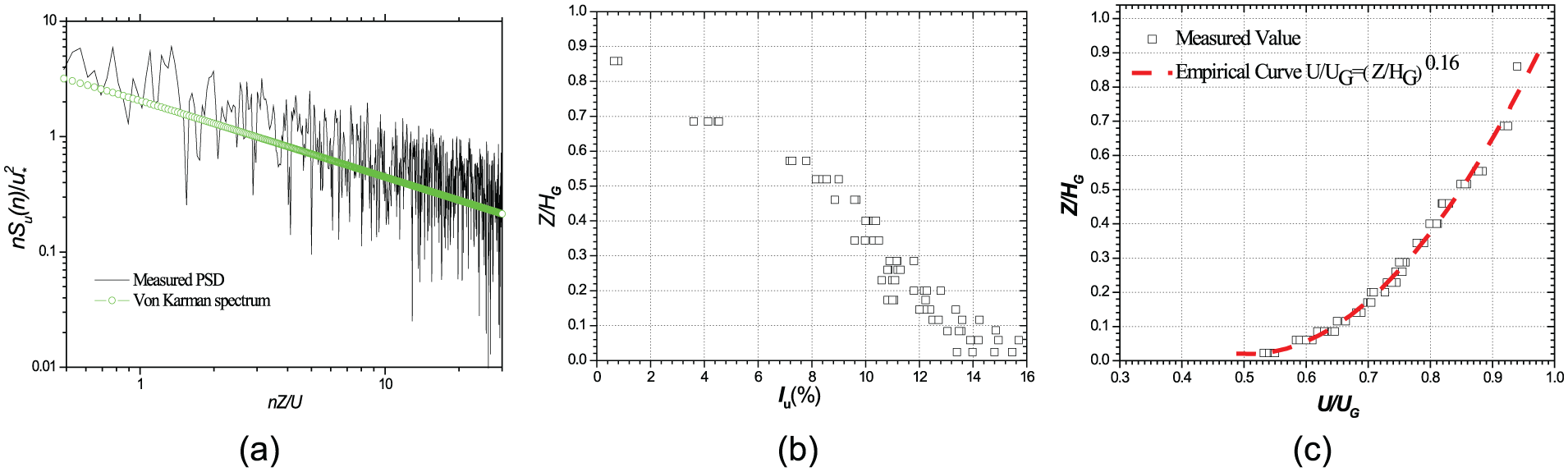
Turbulent flow characteristics for a Type B ABL flow field simulated in a TJ-3 wind tunnel (HG and UG refer to the gradient height and the geostrophic velocity, respectively): (a) power spectral density of along-wind velocity, (b) turbulence intensity profile, and (c) mean wind velocity profile.
As described in section “Aero-elastic model design,” a 1:200 scaled beam-net aero-elastic model is manufactured. Components of the model are thin galvanized sheet steels, the thickness of which is between 0.1 and 1.0 mm. The thickness increment is 0.1 mm. The width direction is processed by means of a linear cutting method, the accuracy of which is 0.01 mm.
Based on the requirements of geometric likelihood, the configuration of the actual cooling tower is simulated by pasting a whole elastic and lightweight membrane tensioned on the outer surface of the steel frame (see Figure 4(a) and (b)). For the beam-net aero-elastic model, the quality of manufacturing is an important issue. Based on the requirement of likelihood, the mass of the steel frame might be insufficient. Thus, the mass is supplemented using copper lead blocks.

Aero-elastic model for pressure and displacement measurements: (a) aero-elastic model, (b) aero-elastic model without outer surface membrane, (c) prototype heights (unit: m) and distribution of pressure measurement points, (d) displacement measurement heights, and (e) pressure measurement points around a horizontal section.
For synchronously measuring pressures and vibrations of the aero-elastic model, each node on the model is equipped with a pressure tap. As shown in Figure 4(c), 36 × 12 taps are uniformly arranged in 12 vertical sections and 36 horizontal circular positions, the distribution of which is shown in Figure 4(e). As shown in Figure 4(d), six heights are equipped with LM10 laser displacement meters (Panasonic Company), the accuracy of which is 0.05 mm for measuring the model’s vibration.
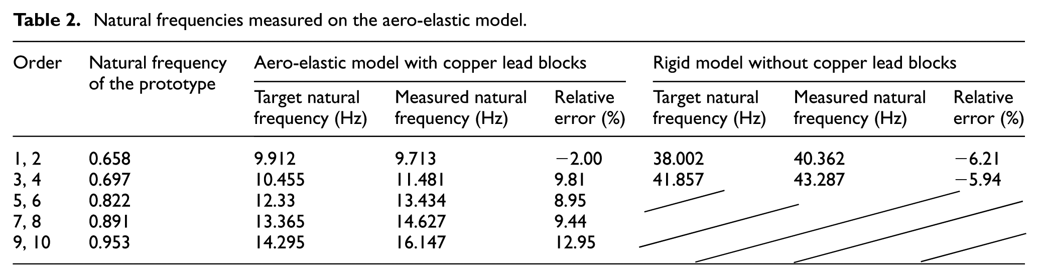
After the aero-elastic model is manufactured, free vibration tests are undertaken to measure low-order natural frequencies, mode shapes, and damping of the aero-elastic model. Excitations are created on the model with regard to the cooling tower’s low-order mode shapes calculated by numerical analyses. The model’s displacement time histories throughout the free vibration process are then recorded using the laser displacement meters. After fast Fourier transforms, displacement power spectral densities are obtained, from which the model’s low-order natural frequencies can be identified. To increase the precision of the free vibration tests, each displacement power spectral density is obtained by averaging the results of five independent runs. The 1st–10th low-order natural frequencies obtained on the model are listed and compared with their simulation targets calculated previously by FE analyses in Table 2. As can be seen, the relative errors for the measured 1st–8th natural frequencies are within ±10%. Besides, the measured structural damping ratio is around 0.024, which falls within the accepted variation range for concrete structures [0.02, 0.05]. These suggest that the dynamic properties simulated on the aero-elastic model agree with those of the prototype. It is noteworthy that the arrangement of pressure tubes may causes some additional structural damping. In this regard, all pressure tubes are attached to the steel tube placed inside the aero-elastic model for arranging the laser displacement meters (see Figure 4(a)). Through this way, the influence of the pressure tubes to the vibrations of the aero-elastic model can be greatly reduced. Besides, when the free vibration tests are undertaken for estimating the structural damping, the pressure tubes are already arranged on the aero-elastic model. So the measured structural damping ratio includes the effect of pressure tubes, and there is no need to eliminate the effect of shaking of pressure tubes when the structural damping ratio is correctly simulated.
Natural frequencies measured on the aero-elastic model.
Effects of Reynolds number (Re) are important for estimating wind loads on curved models. The difference in Re between the wind tunnel test of an object and the full-scale situation results in different flow characteristics, which can cause inaccuracies in the wind tunnel simulations. Fortunately, Re is not the only factor that influences the fluid flow. Surface roughness of the test body is also an important influence. And it is widely acknowledged that at a high Re the mean wind pressure distribution around a circular cylinder can be reproduced at lower values of Re with a suitable roughening of the surface of the round body (Lawson, 1982). After comparing several types of surface roughness, attaching 36 uniformly distributed three-layered vertical paper tapes with a test wind speed of 8 m/s was identified to be the optimal approach to simulate the effects of a high Re. As shown in Figure 5, the mean wind pressure distribution measured on the rigid model with the optimal Re effects simulation approach and the full-scale measurement data reported by the Chinese Code GB/T 50102-2003 (2003) are close to each other.
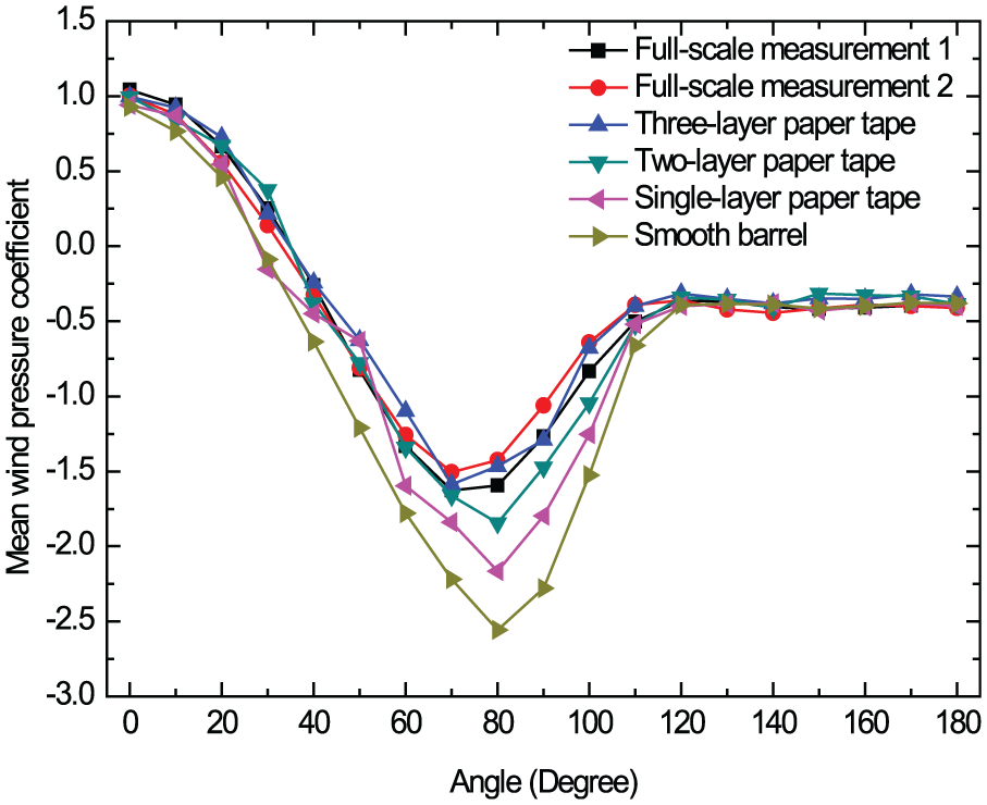
Mean wind pressure distributions for different Re effects simulation measures on the rigid model.
The LRC method
Basic theory
For the maximum of a response
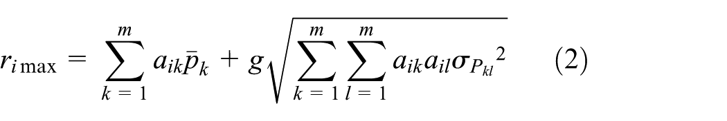
with
Equation (2) can be rewritten as
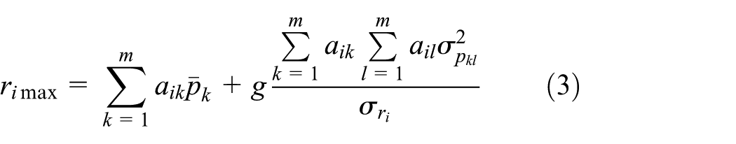
in which
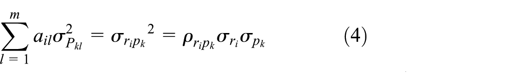
with
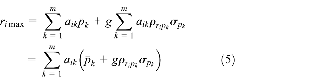
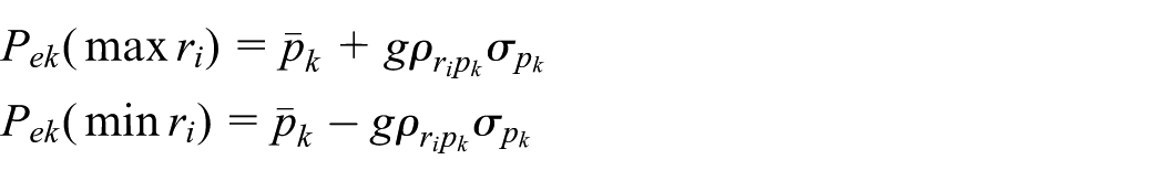
The load pattern given within parentheses in equation (5) is defined as the sum of the mean load and a weighted fluctuating load. The weighting factor is the correlation of the load and the response. Thus, it is called the LRC method. Used in the sense of an ESWL, this load pattern accurately produces the peak response of a linear system (Kasperski and Niemann, 1992). Thus, for a specific response

Application of the LRC method
In practice, ESWL calculations based on the LRC method can be realized with the following steps:
Choose the reaction
Use wind tunnel experiments to obtain wind pressure samples
Calculate the statistic parameters of the load, for example, the vector of mean values
Based on the FE analyses, calculate the influence factors
Calculate the standard deviation of each response
Calculate the correlation of load and response:
Calculate the peak factor:
Calculate the ESWL distributions
In the above, steps 5 and 6 are based on the assumption of linearity, and step 7 is based on the assumption of Gaussian distribution.
Comparison of results
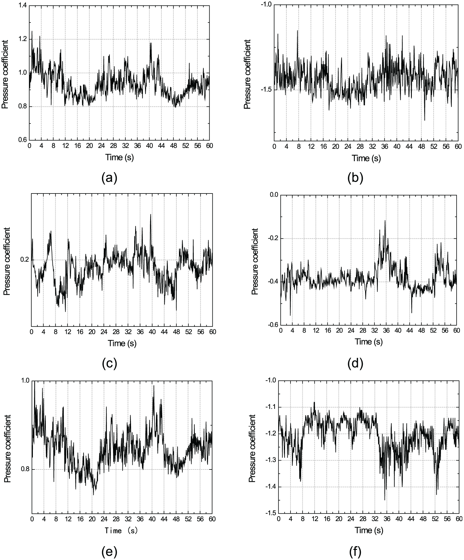
After data processing, six wind pressure load samples (LS) and six wind-induced displacement response samples (RS) are simultaneously measured on the aero-elastic model (see Figures 6 and 7(a), (c), (e), (g), (i), and (k), respectively), which takes into account the structure’s non-linearity and the non-Gaussian properties of wind loads. Besides, fast Fourier transforms are undertaken for the time history samples presented in Figure 7, and the amplitude spectral densities obtained (Figure 7(b), (d), (f), (h), (j), and (l)) suggest that the large cooling tower is a quasi-static structure, since no spikes can be observed in the amplitude spectral densities at the structure’s natural frequencies.
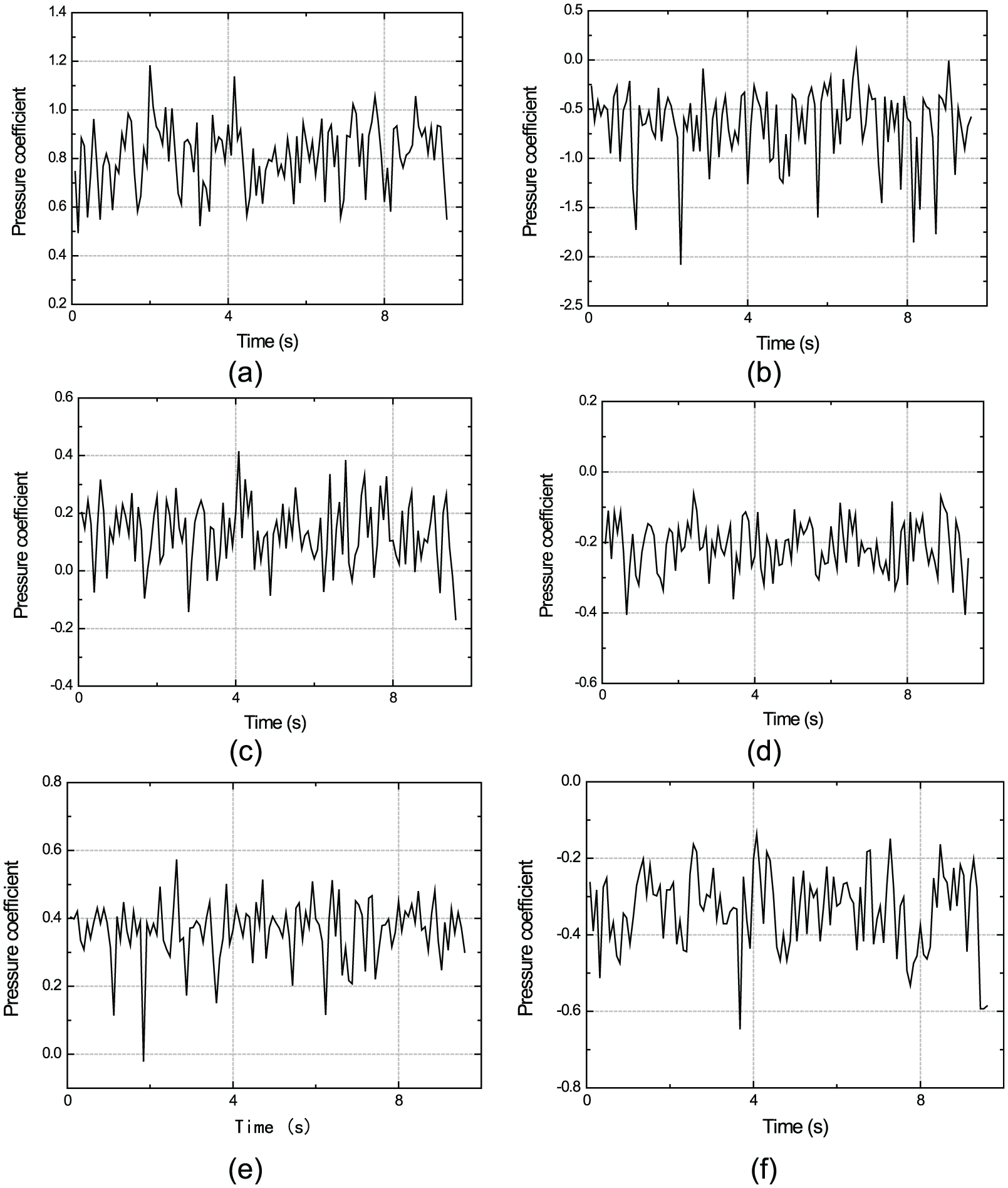
Wind pressure time histories measured on the aero-elastic model: (a) LS1 (sec. 2—no. 1), (b) LS2 (sec. 4—no. 9), (c) LS3 (sec. 7—no. 4), (d) LS4 (sec. 8—no. 16), (e) LS5 (sec. 12—no. 2), and (f) LS6 (sec. 8—no. 7).
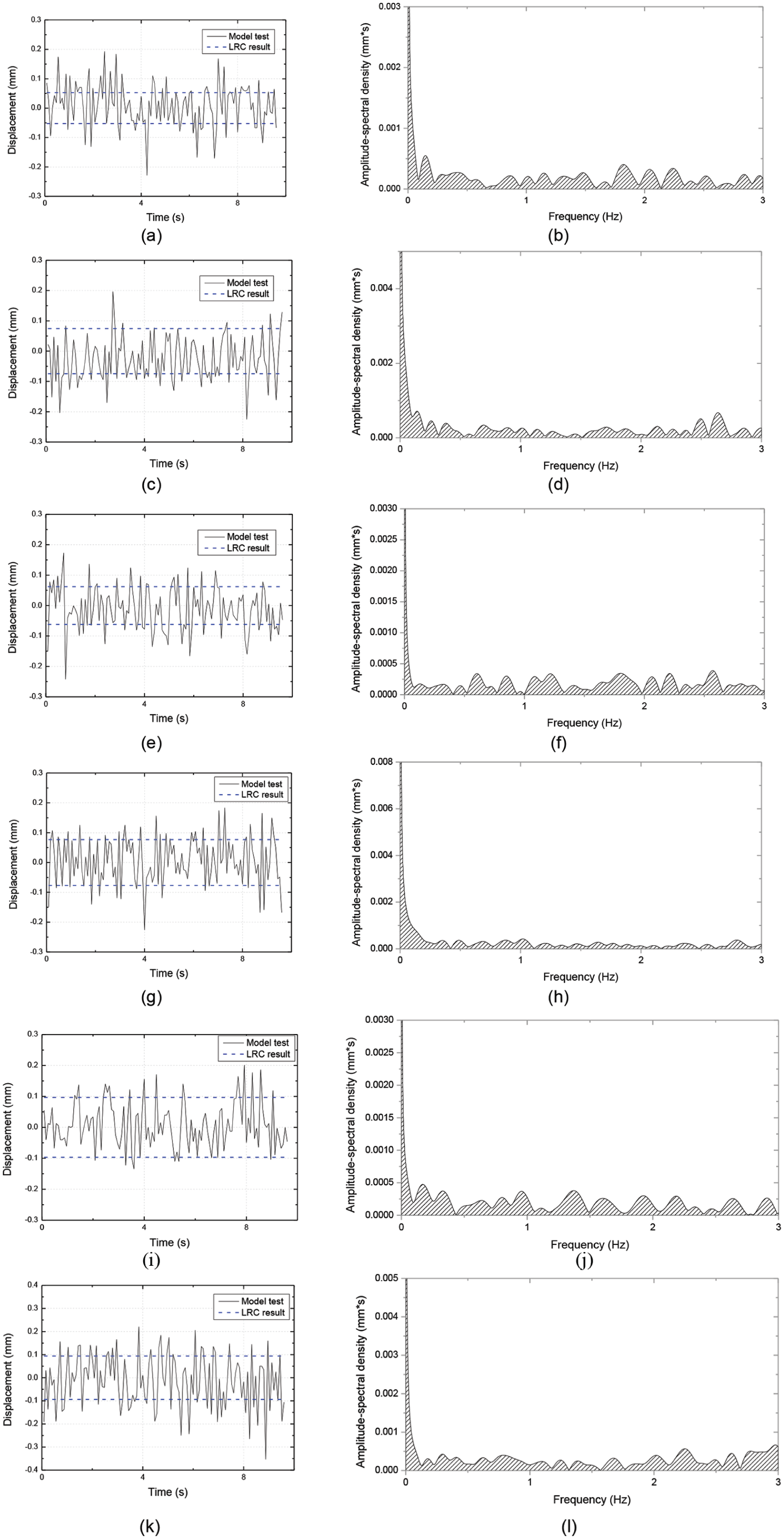
Wind-induced displacement responses measured on the aero-elastic model: (a) time history for RSa (sec. 1—no. 1), (b) amplitude spectral density for RSa (sec. 1—no. 1), (c) time history for RSb (sec. 1—no. 3), (d) amplitude spectral density for RSb (sec. 1—no. 3), (e) time history for RSc (sec. 4—no. 1), (f) amplitude spectral density for RSc (sec. 4—no. 1), (g) time history for RSd (sec. 4—no. 4), (h) amplitude spectral density for RSd (sec. 4—no. 4), (i) time history for RSe (sec. 6—no. 1), (j) amplitude spectral density for RSe (sec. 6—no. 1), (k) time history for RSf (sec. 4—no. 7), and (l) amplitude spectral density for RSf (sec. 4—no. 7).
Some correlation coefficients between LS presented in Figure 6 and RS presented in Figure 7 are calculated. Besides, the correlation coefficients are calculated correspondingly based on the LRC method. Figure 8 shows the comparison of the measured correlation coefficients and the calculated ones. As shown in Figure 8, the trends of variation are the same for the measured correlation coefficients and the calculated ones. However, the correlations are generally stronger for LRC calculation than for wind tunnel measurement. The correlation coefficients for the LRC calculation are 1.5–6 times those for wind tunnel measurement. It is found that when the distance between the load position and the response position gets farther, the result based on the LRC calculation gets closer to the exact result based on wind tunnel measurement (e.g. LS3/RSa, LS4/RSa, and LS5/RSa correlation coefficients). Moreover, the peak responses calculated by LRC are adjusted for length scaling of the model test and shown in Figure 7(a), (c), (e), (g), (i), and (k). The comparisons between the model test results and the LRC results in Figure 7 clearly suggest that the LRC method is generally conservative for use.
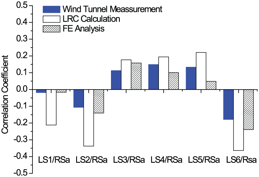
LS/RS correlation coefficients based on wind tunnel measurement, LRC calculation, and FE analysis.
Non-linear FE analyses applying realistic non-Gaussian wind pressure field
Although the aero-elastic model test described in section “Wind tunnel model test” is reliable, it should be acknowledged that all physical experiments are subjected to inherent uncertainties. Thus, we suppose that an accurate FE analysis, which takes into account the non-linearity of the real structure and the non-Gaussian feature of the actual wind loads, is required for validating the model test results presented above.
The 215-m-high cooling tower is modeled again based on a commercially available FE platform. This time, the tower shell is discretized into 324 solid elements and 36 pairs of herringbone columns are modeled by beam elements (see Figure 9). The solid element is for three-dimensional (3D) modeling of concrete with the reinforcement behavior. It can reflect the cracking of concrete in tension, the crushing of concrete in compression, as well as the plastic deformation. The cracking stress and the crushing stress for the concrete are set at 3 and −30 MPa, respectively. The solid element can also reflect the tension and the compression of the reinforcing bars. The most important aspect of this element is the treatment of non-linear material properties. The yield criteria used for establishing the model are shown in Figure 10.
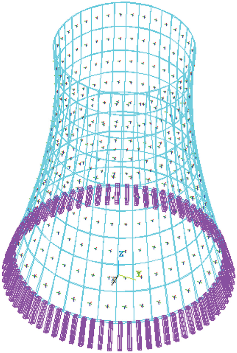
The non-linear FE model with geometries displayed as outlines.
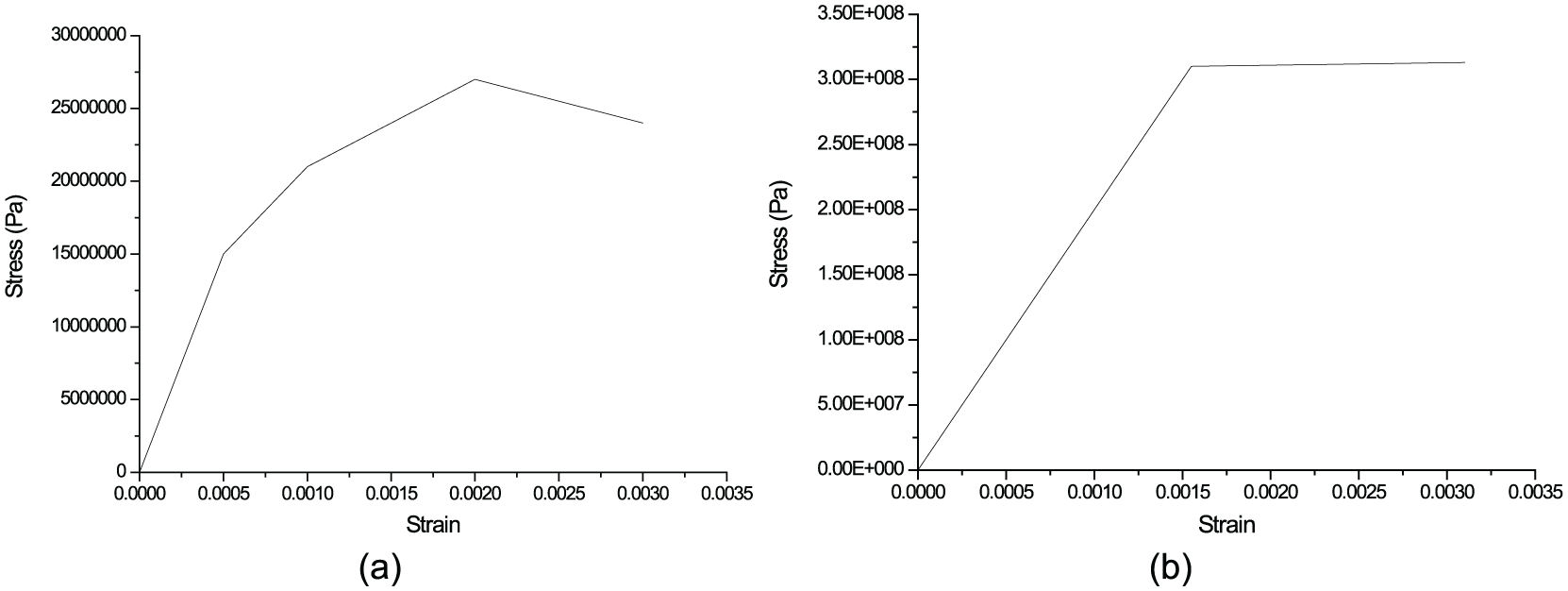
Yield criteria for (a) concrete and (b) reinforcement.
Wind pressure data measured at the throat section of Peng-cheng cooling tower (Cheng et al., 2015) are utilized for the analyses. According to Cheng et al. (2015), all wind pressure samples obtained around the half-circle of Peng-cheng cooling tower follow non-Gaussian distributions. Fluctuations of wind pressure coefficients at other heights are assumed to be identical to those of the throat section, so data on the whole surface are obtained. A time-domain approach, namely, Newmark-β method, including large-deflection effects, is used to calculate the structural dynamic responses. Six wind pressure samples employed for the non-linear FE analysis are shown in Figure 11. The wind-induced displacement time history and the corresponding power spectral density are calculated at the position corresponding to RSa (see Figure 12). The correlation coefficients between LS presented in Figure 11 and the RS presented in Figure 12 are added in Figure 8. As shown in Figure 8, the FE analysis results are close to the aero-elastic model test results, suggesting that the physical experiment described in section “Wind tunnel model test” is reliable.
Wind pressure time histories measured on Peng-cheng cooling tower (the circumferential positions where LS1–LS6 are measured are the same as in Figure 6): (a) LS1, (b) LS2, (c) LS3, (d) LS4, (e) LS5, and (f) LS6.
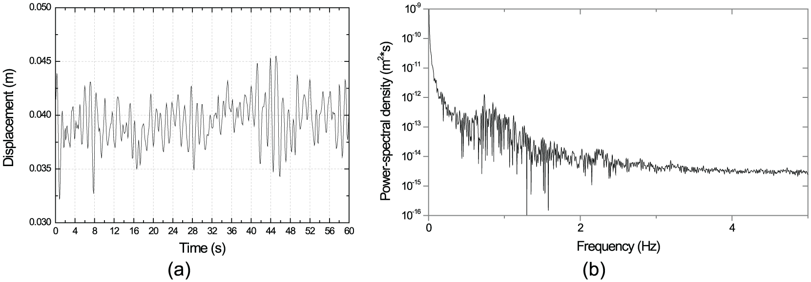
Wind-induced displacement time history calculated at the position corresponding to RSa in Figure 7: (a) time history and (b) power spectral density.
Conclusion
The conclusions of this study concerning the application of the LRC method to ESWL calculation for large cooling towers are summarized as follows:
An innovative beam-net aero-elastic model is designed for a large cooling tower to simultaneously produce wind loads and wind-induced displacements of the structure in the wind tunnel. Besides, a non-linear FE analysis applying the non-Gaussian wind pressure field measured on a full-scale large cooling tower is also conducted to validate the wind tunnel model test. A comparison between LRC coefficients measured on the scaled model and results based on the FE analysis suggests that the wind tunnel model test is reliable.
LRC coefficients are generally larger for the LRC calculation than for the exact wind tunnel measurement. This is because the non-linearity of the real structure and the non-Gaussian feature of the actual wind loads weaken the correlations between the wind loads and the structural responses.
The variation trends of correlation coefficients on the entire tower surface are basically the same between the LRC calculation and the exact wind tunnel measurement. Thus, LRC can be applied to ESWL calculation for large cooling towers. However, since direct applications of the LRC method to large cooling towers might lead to too conservative structural designs, we recommend that a multiplier is employed to reduce the correlation coefficients calculated based on LRC method in the case that the load position and the response position are very close.
Footnotes
Declaration of Conflicting Interests
The author(s) declared no potential conflicts of interest with respect to the research, authorship, and/or publication of this article.
Funding
The author(s) received no financial support for the research, authorship, and/or publication of this article.