
Abstract
The accurate estimation of natural frequencies and damping ratios is critical for civil structures. In this article, a method based on short-time narrow-banded mode decomposition is proposed to analyze the modal parameters of civil structures. In this approach, short-time narrow-banded mode decomposition is applied to identify time-varying structures with free vibration responses. On the contrary, by analysis of the weighting factors α and β, short-time narrow-banded mode decomposition is improved to estimate the parameter of time-invariant systems. In the case of enhanced short-time narrow-banded mode decomposition, the original short-time narrow-banded mode decomposition approach is modified in two ways. First, the instantaneous frequency term of the objective function is removed, and one weighting factor remains, that is, α in the objective function. Second, a technique is provided to automatically detect the optimum value of α. Two numerical examples, that is, a three-degree-of-freedom time-variant system and a simple model of the Lysefjord bridge are provided. In addition, an experiment with a real-life pedestrian bridge located at Tufts University, United States, is used to demonstrate the applicability of the proposed method. The analysis results indicate that the proposed method can easily identify high-quality natural frequencies and damping ratios.
Keywords
Introduction
Civil structures may be damaged, deteriorated, and destroyed by severe earthquakes, strong winds, hurricanes, and fatigue load due to ambient vibration. To avoid economic and human losses, early damage detection and reinforcement are vital. In this regard, modal parameter identification (MPI), especially natural frequencies and damping ratios, of civil structures has demonstrated to be critical because these parameters can reflect vibration characteristics (Rainieri et al., 2018). MPI has been extensively applied in damage detection (Magalhães et al., 2012), modal updating (Bagheri et al., 2018), vibration control (Bakule et al., 2016), and seismic design (Muho et al., 2019). Because operational modal analysis is practical and inexpensive, an increasing number of researchers are exploring techniques using ambient vibration (Amezquita-Sanchez et al., 2017).
Recent advances in signal processing algorithms have stimulated the development of MPI. Distinct methods reflect the diverse characteristics of a signal, based on which the algorithms can be classified into time-domain algorithms, frequency domain algorithms, and time–frequency domain algorithms (Xu et al., 2002). Frequency domain decomposition (Brincker et al., 2001), the peak-picking method (Ren et al., 2004), and enhanced frequency domain decomposition (Jacobsen et al., 2006) are examples of frequency domain algorithms. Frequency domain algorithms have a few common limitations; for example, they are not suitable for signals with a low signal-to-noise ratio (SNR) and closely spaced modes (Bagheri et al., 2018). Many time-domain algorithms exist, such as stochastic subspace identification (SSI; Peeters and De Roeck, 1999), the natural excitation technique combined with the eigensystem realization algorithm (NExT-ERA; Caicedo et al., 2004), and the random decrement technique combined with the Ibrahim time domain (RDT–ITD; Ibrahim, 1977; Ibrahim and Pappa, 1982). Although outstanding results can be obtained using the SSI, RDT-ITD, and NExT-ERA techniques, several challenges remain. For example, SSI and NExT-ERA typically require high-order modes when testing closely spaced modes, which might lead to spurious or false frequency elements (Perez-Ramirez et al., 2016). In addition, empirical mode decomposition (EMD; Yang et al., 2003a), which is a well-known algorithm, is a time-domain method. Regarding EMD, the lack of a theoretical mathematical basis leads to several issues; the main hindrances, such as (a) the unpredictable or varying number of modes, (b) the end effects of the spline curve, (c) the nonstandard sifting stopping criterion, and (d) the lack of orthogonality and mixing of the mode results, are described in McNeill (2016). Several time-frequency domain methods, including the wavelet transform (WT; Le, 2017) and Hilbert–Huang transform (HHT; Yang et al., 2004), are also used to identify the structural modal parameters. Unfortunately, the abilities of WT and HHT decrease when analyzing the signals of civil structures because noise is inescapable. Moreover, the freedom in the selection of the mother wavelet function may cause a marked disturbance, which may produce poor or inaccurate results when the choice of the mother wavelet function is erroneous or improper (Qin et al., 2018). The core of the HHT algorithm is EMD and its performance influences the results of the HHT (Amezquita-Sanchez and Adeli, 2016).
To reduce certain imperfections, several methodologies for MPI have been proposed in recent years. Proposed by Daubechies et al. (2011), the synchrosqueezed wavelet transform (SWT) is a combination of the WT and reallocation methods. The SWT was introduced to MPI in combination with the Hilbert transform (HT) and Kalman filter by Perez-Ramirez et al. (2016). The SWT-based methodology can analyze noisy and closely spaced mode signals and improves the accuracy of the estimated modal parameters. The mother wavelet function varies, and distinct choices produce different results. Furthermore, the parameters of the Kalman filter, which depend on the characteristics of the sensors that are utilized to obtain the signals, are not practical. The empirical wavelet transform (EWT), which was proposed by Gilles (2013), is similar to a wavelet filter bank for extracting monomodes. For the EWT, obtaining the segments of the Fourier spectrum is essential because these segmentations affect the accuracy of calculations. With this method, a low SNR and closely spaced mode signals may present an immense challenge to the EWT. Although the power spectrum has been employed to improve the EWT in recent work (Amezquita-Sanchez et al., 2017; Luo et al., 2018; Xin et al., 2019), the influence caused by the transition zone cannot be eliminated. Thus, closely spaced modes would not be well separated by the EWT. Recently, variational mode decomposition (VMD), which was proposed by Dragomiretskiy and Zosso (2014), was applied to MPI by Bagheri et al. (2018). The VMD method decomposes a signal into a set of distinctive subsignals with a center frequency contained in each subsignal. The algorithm is entirely nonrecursive and has outperformed the EMD approach. However, VMD has no capacity for estimating modes with a small amplitude, especially when the predominant elements have broad spectral tails (McNeill, 2016). In addition, VMD is inappropriate for a signal with a low SNR or closely spaced modes.
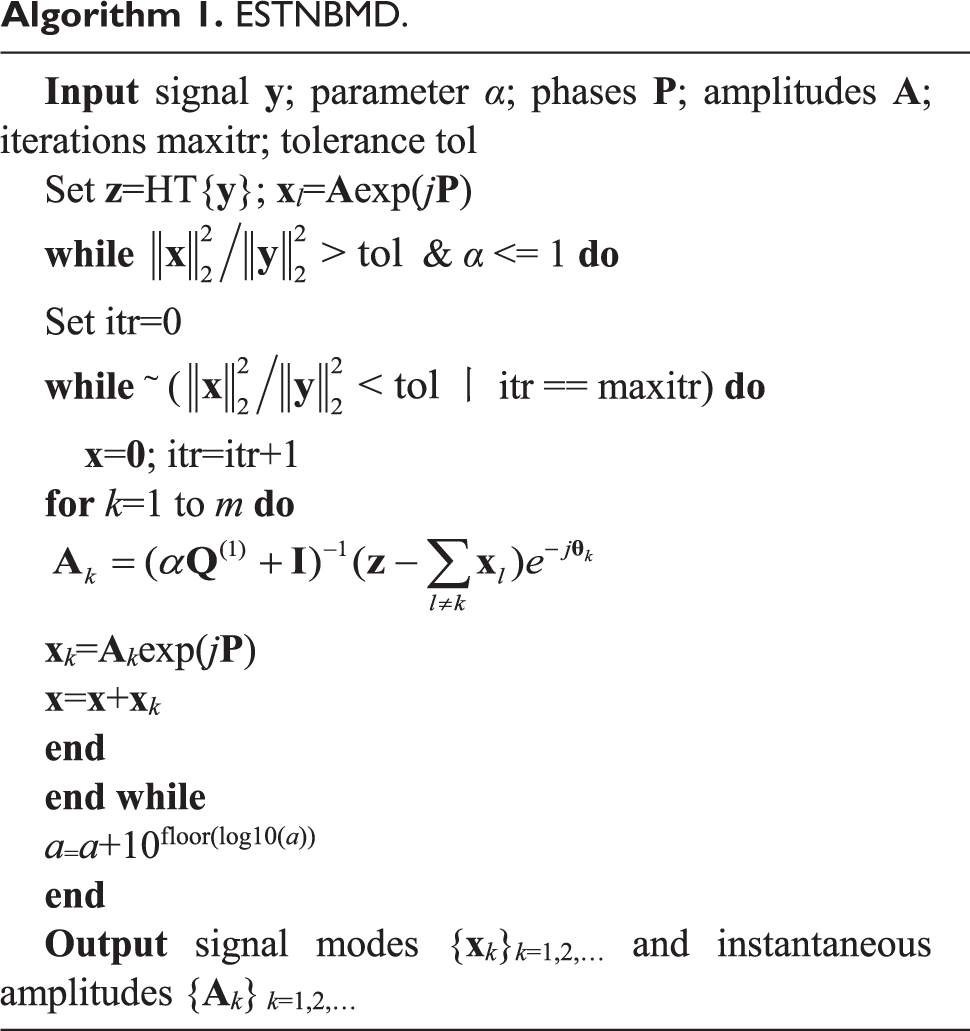
Recently, McNeill (2016) introduced a novel algorithm that is referred to as short-time narrow-banded mode decomposition (STNBMD). This method decomposes a signal into a set of short-time narrow-banded components and the sum of the monocomponents reproduces the original signal. The STNBMD algorithm has an excellent theoretical principle, which uses a series of suboptimal updates of phase and amplitude to approach the minimum of a target function. This algorithm is a simple, nonparametric, and efficient signal processing technique. However, determining the weighting factors α and β in the STNBMD algorithm is difficult, and no criterion exists for optimal weighting factors.
In this article, based on the feature of time-invariant structures that natural frequency is nearly constant, an enhanced STNBMD (ESTNBMD) method is introduced. We have modified the original STNBMD method in two ways. First, the instantaneous frequency term of the objective function is removed, and one weighting factor remains, that is, α in the objective function. Second, we have provided a technique for automatically detecting the optimum value of α. Last, we proposed a method for the MPI of structures based on STNBMD and ESTNBMD.
The remainder of this article is organized as follows: First, the theoretical background of the primary STNBMD method and its development are given in section “Theoretical background and development.” Second, section “Methodology” briefly describes the methodology of structural MPI based on STNBMD in time-variant systems and ESTNBMD in time-unvarying structures. Third, in section “Numerical studies and verification,” a time-variant three-degree-of-freedom (DOF) system and a simple model of the Lysefjord bridge are simulated to validate this proposed method. In section “Experimental study and validation,” an experiment of a real-life pedestrian bridge located in Tufts University, United States, that is measured using ambient vibration is employed to confirm the effectiveness of the proposed method. Last, the main conclusions of this article are addressed in section “Concluding remarks.”
Theoretical background and development
Original STNBMD algorithm
The STNBMD algorithm aims to decompose an analytical raw signal into several component modes with slowly varying amplitudes and phase angles. This algorithm can be divided into two parts: HT analysis, which obtains the analytical signal and objective function minimization (McNeill, 2016). The details of each part are described as the following.
HT
The first step of the STNBMD method is to obtain the analytical signal of the measured data using the HT. This transform was proposed by Hilbert (1912) and calculates the time series u(t) by convoluting u(t) with the term 1/t as
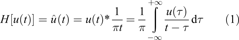
where

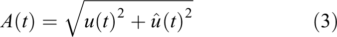
where j is the imaginary portion of the analytical signal z(t). A(t) and θ(t) are the envelope of u(t) and phase of u(t), respectively, which are defined as follows

Objective function minimization
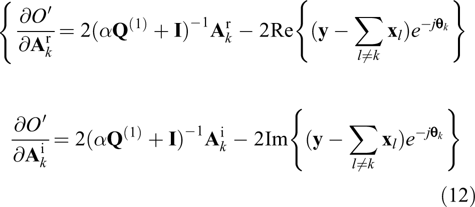
The core of the STNBMD algorithm is to decompose the analytical signal into constituent modes by minimizing the objective function. This objective function contains three terms: the first term forces the slow variation of the instantaneous amplitude envelope, the second term compels the instantaneous frequency to vary slowly, and the last term is the error between the original data and the reconstructed signal. The objective function is written as
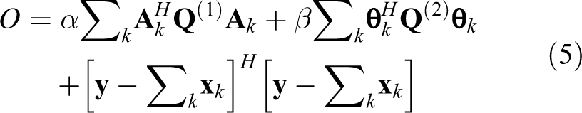
where
where
and the superscripts r and i in equations (6) and (7) indicate the real portion and imaginary portion, respectively.
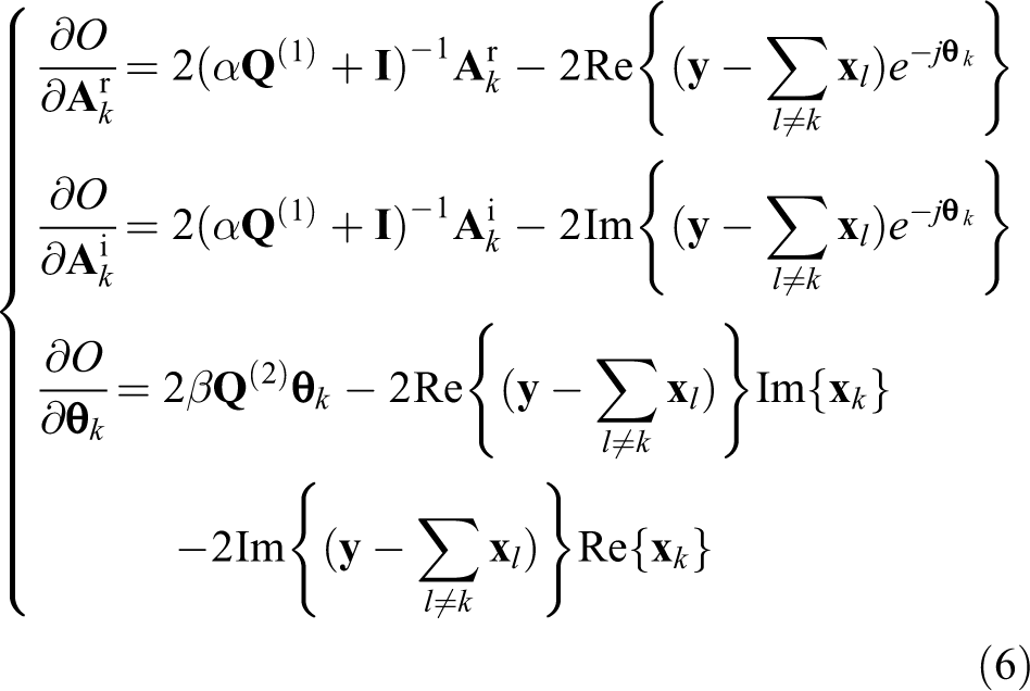
The minimum occurs at the stationary point, where the gradient of the objective function equals zero. The STNBMD method uses a suboptimal update optimization method that is similar to that in Dragomiretskiy and Zosso (2014). Moreover, the update rules of the amplitudes and phases are applied to approach the stationary point as

where
Analysis of weighting factors α and β
It can be known from equation (5) that α and β control the smoothness of amplitude and frequency, respectively. When one of the terms is smoother, it will have a smaller impact on the objective function, that is, the corresponding weight factor in the appropriate range will also influence it slightly. For example, we apply the STNBMD to a linear time-invariant system. The frequency change of this system is close to zero, that is,
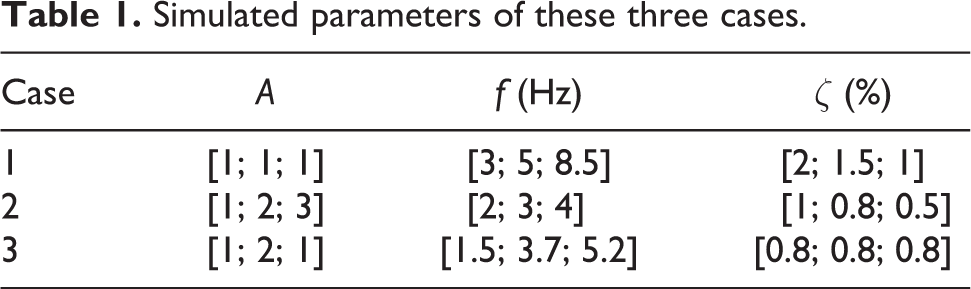
To know the best value of the weighting factors in the STNBMD method, three 3-DOF damped free vibration responses (FVRs) are employed (Yan and Miyamoto, 2006)
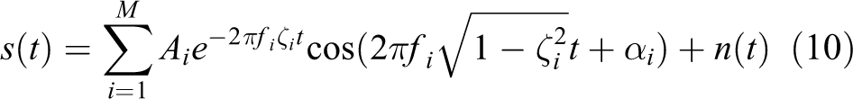
where s (t) is a synthesized signal, Ai is the amplitude, fi is the natural frequency, ζi is the damping ratio, αi is the phase angle of the ith monocomponent, M is the number of components i, and n(t) represents the intensity of white noise. The phase angles of these three signals are set to 0; the other parameters are shown in Table 1. For example, in case 1, the three natural frequencies—f 1 = 3, f 2 = 5, and f 3 = 8.5 Hz—have amplitudes of 1, and the correlated damping ratios are ζ 1 = 2%, ζ 2 = 1.5%, and ζ 3 = 1%. In this simulation, a sampling frequency of 200 Hz is applied to yield 1000 samples within a time window of 5 s.
Simulated parameters of these three cases.
STNBMD is applied to these signals. As the feature of simulation signals, that is, the instantaneous amplitude changes are more dramatic than the instantaneous frequency. As mentioned above, the weighting factor of α will dominate the objective function. Moreover, according to the weighting factors used in STNBMD (McNeill, 2016), the ranges of α and β are set to [1.0e−3, 1.0e0]. To show the results of the influence of weighting factors, 28 times are calculated in this simulation. As shown in Figure 1, α is gradually increased from 1.0e−3 to 1.0e0 each time by the smallest number of the same-order number magnitude and β is set to 1.0e−3 in each time. For other parameters, the number of iterations is 100, the convergence tolerance is 1.0e−6, and the values of the initial frequencies are set to fi to eliminate the initial value effect.
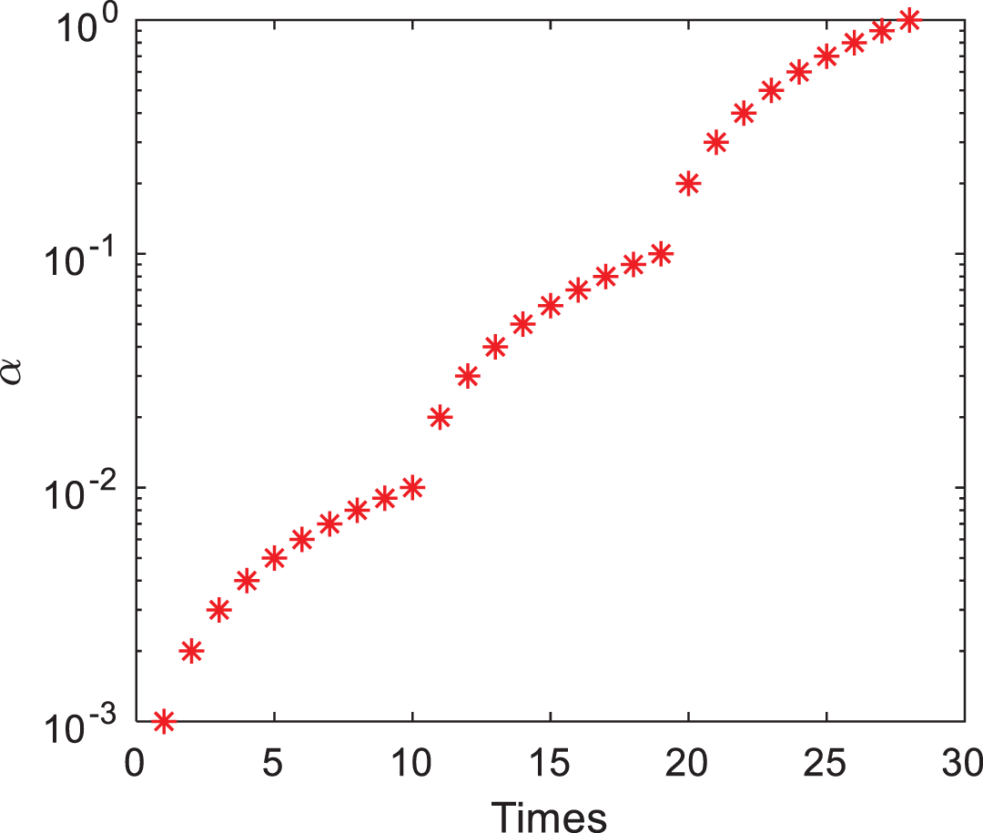
Weighting factors α in each time.
Figure 2 shows the mean error between the instantaneous amplitude of both the restructured signal and the primitive signal, and the convergence index (0 indicates that convergence has not been achieved, and 1 represents convergence). The mean error reveals that the high values of α may achieve better results than the lower values, which shows agreement with the suggestion in the literature (McNeill, 2016): for the best scheduling, the values of the weighting factors are determined from high values to lower values. However, when using this suggestion, defining the best result is difficult. First, high values of the weighting factors will cause the modal amplitudes overly smoothed (McNeill, 2016). This phenomenon, revealed in Figure 2, is that the mean error increases with α after the convergence. Second, lower values of the weighting factors cannot achieve convergence in the STNBMD. Nevertheless, the minimum values of the mean error and the turning points of the convergence index from 0 to 1 are equivalent in the three cases. In general, the smallest mean error means that the restructured results are optimal. Therefore, α, which corresponds to the turning point of the convergence index, can be regarded as the best setting when the instantaneous frequency is smoother than the instantaneous amplitude.
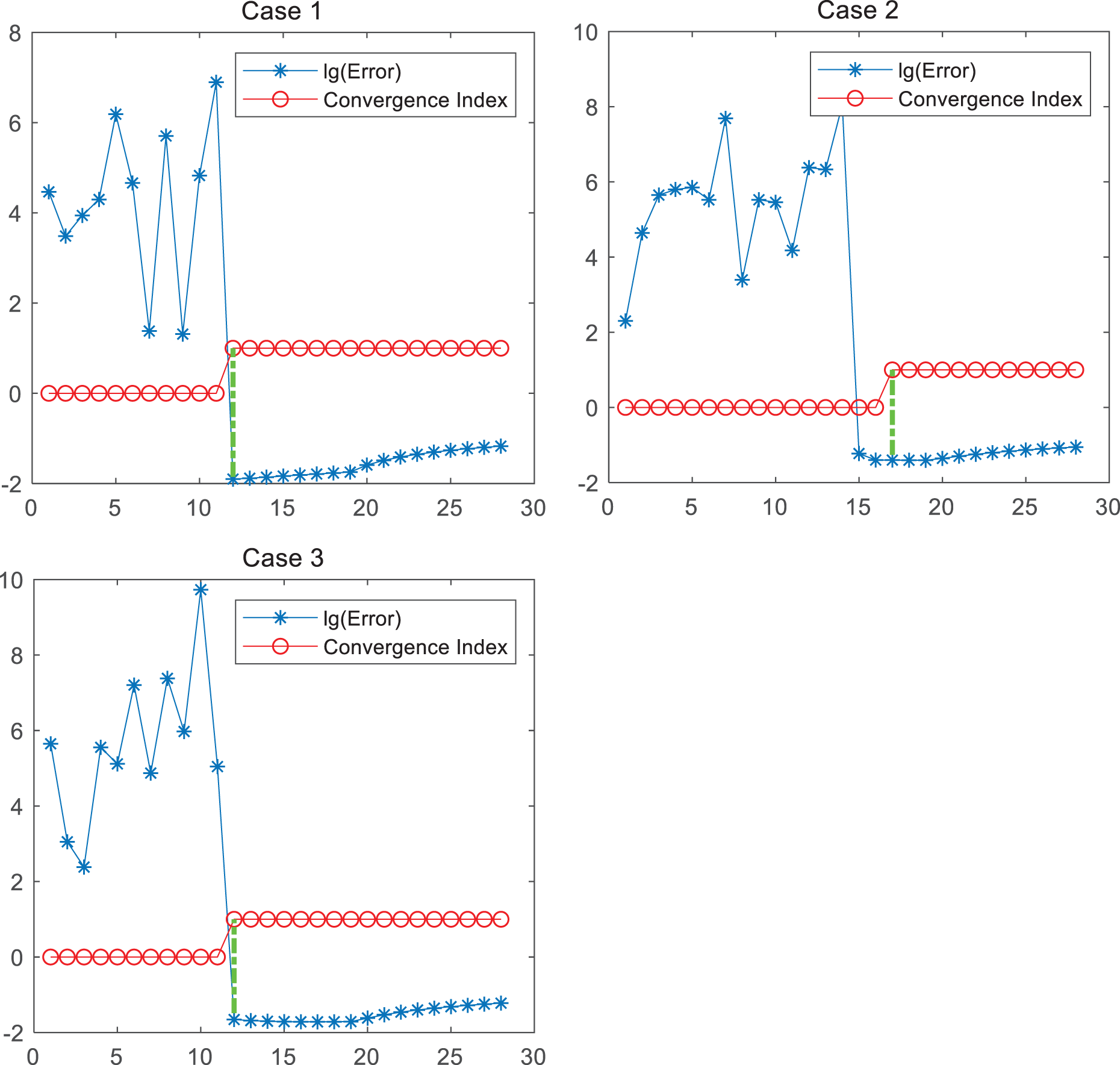
Mean error between the restructured signal and the original signal, and the convergence index (0 indicates that convergence has not been achieved, and 1 represents convergence) in these three cases.
ESTNBMD approach
As shown in the literature (McNeill, 2016), choosing the weight factors α and β is a considerable challenge to application of the STNBMD method. Using the properties of the structural vibration signals of the time-invariant structures and the traits of the weighting factors of the STNBMD approach, an ESTNBMD method is developed in this subsection.
Removing the instantaneous frequency term of the objective function
As time-unvarying structures, the natural frequencies are almost constant. Therefore, the second term of the original objective function can be eliminated when the initial frequencies are similar to the true modes. The new objective function is given as follows
The gradient is constructed as follows
Equation ( 8) expresses the update rules.
Automatic detection of the optimum weighting factor α
Using the results from the analysis of the weighting factors, the ESTNBMD method would automatically find the optimal weighting factor α by detecting the turning point of convergence. The initial value α is set to 1.0e−3 and gradually increases (shown in Figure 1) when the result has not converged. We recommend setting the number of iterations to 100 and the convergence tolerance to 1.0e−6. The same parameters are chosen for the ESTNBMD method in the following cases. Algorithm 1 summarizes the framework of the ESTNBMD method.
ESTNBMD.
Methodology
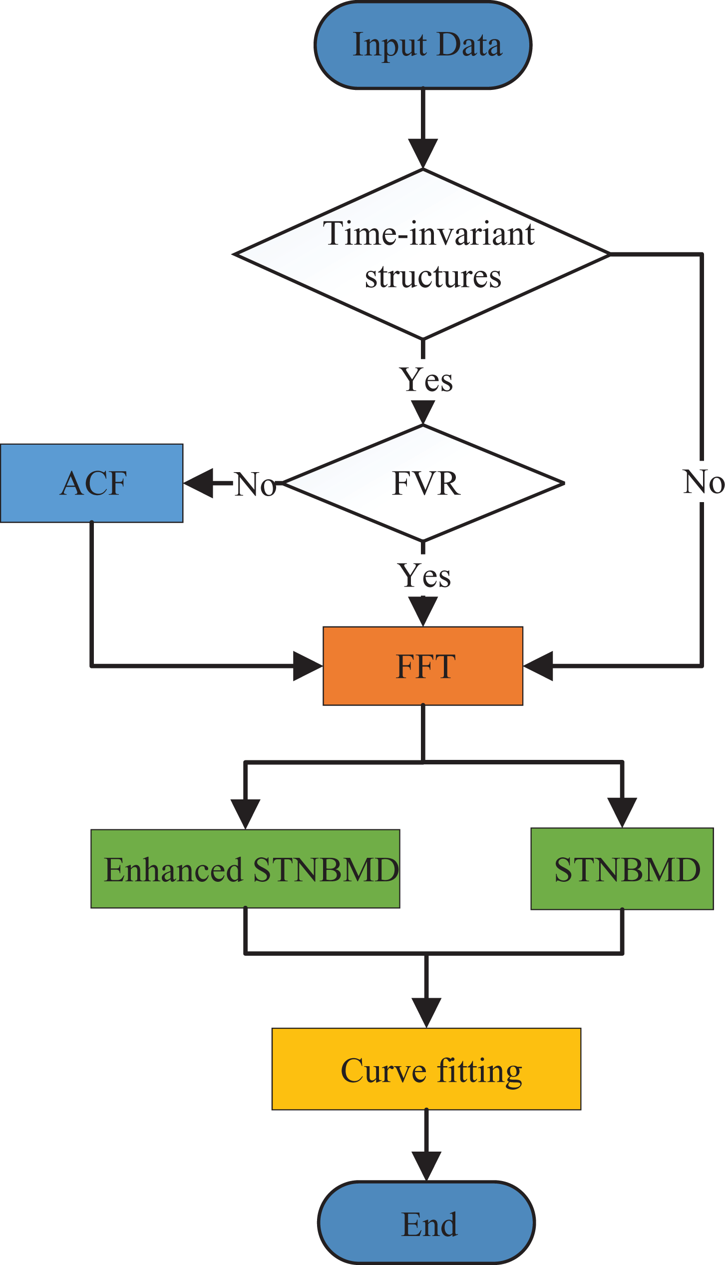
In this article, we focus on the application of ESTNBMD to time-invariant structures and the application of STNBMD to time-varying systems with a FVR. The main steps of parameter identification are described as follows.
Time-invariant structures
First, the vibration responses are obtained from structures. If these data are ambient responses, the autocorrelation function (ACF; Vandiver et al., 1982) is used to extract the FVR. The ACF can be characterized by the following equation
where the input xt
is defined as a stochastic process, which consists of a finite time series of x
1, x
2,…, xN
of N observations; x
t+m
is a lagged version of xt
, where m = 0, 1,…, M;
Before the application of the ESTNBMD algorithm, the Fast Fourier transform (FFT) is applied to estimate the frequencies (fk ) of the FVR. The FFT provides excellent results in terms of the frequency resolution, especially when there is no noise exist in the FVR. Moreover, the ESTNBMD method is used to analyze the FVR and the estimated frequencies as the initial values for its calculation.
Once the instantaneous amplitude

where a is the product of damping ratio and the undamped modal frequency, and b is a constant. According to equation (14), by plotting the decaying form amplitude ln(
Time-varying systems
For time-varying systems, the STNBMD should be applied; its process of identification is similar to that of time-unvarying structures. However, the natural frequencies and damping ratios are different. Natural frequencies of systems are obtained from the instantaneous phase angle
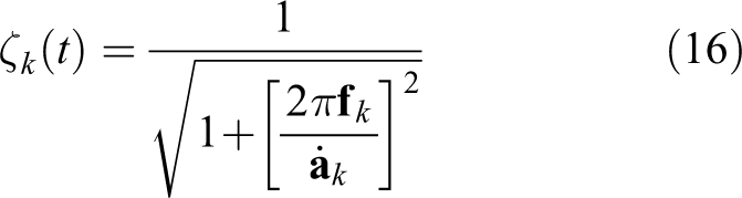
where
The previously mentioned identification process is summarized in Figure 3.
Illustrative diagram of the procedures referred to in the introduced method.
Numerical studies and verification
A time-varying 3-DOF system
To illustrate the effectiveness of the proposed method, a time-variant 3-DOF system is employed, as shown in Figure 4. The mass coefficients of the system are set as mi
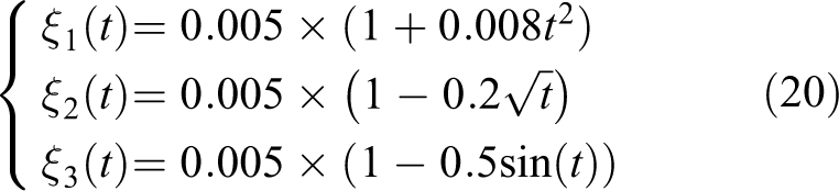
= 8 kg (i = 1, 2, 3), which is associated with the time-varying stiffness coefficient
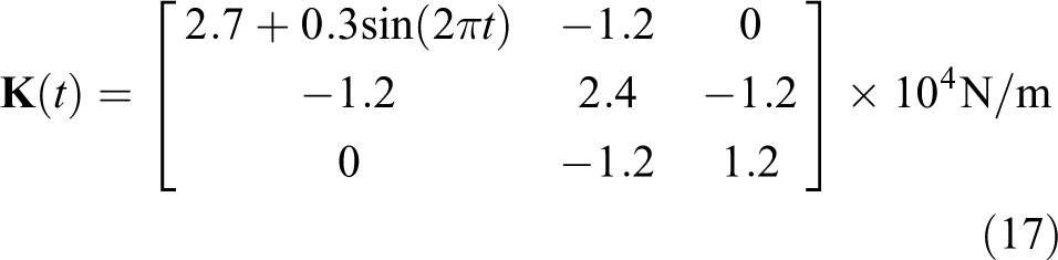
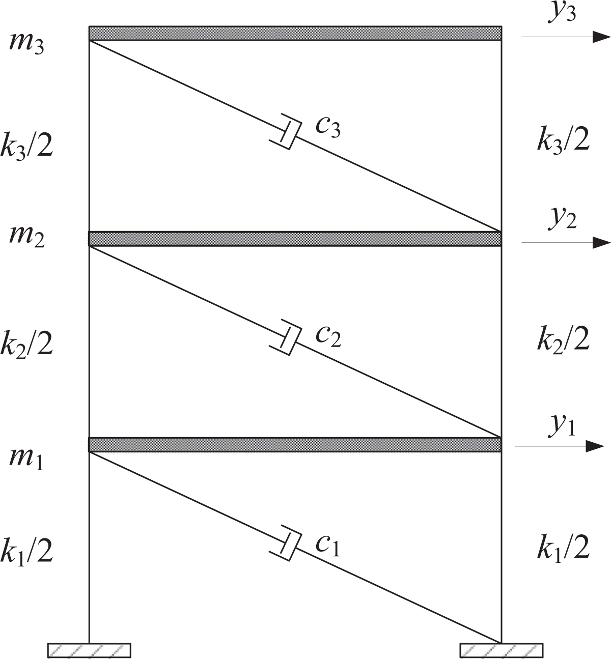
A time-variant 3-DOF system.
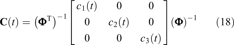
where ck
(t) = 2ζk
(t)ωk
(t)Mk
, and
In the process of simulation, this system is calculated by the fourth-order Runge–Kutta method and a time window of 10 s with a sampling frequency of 200 Hz.
In this example, the acceleration responses
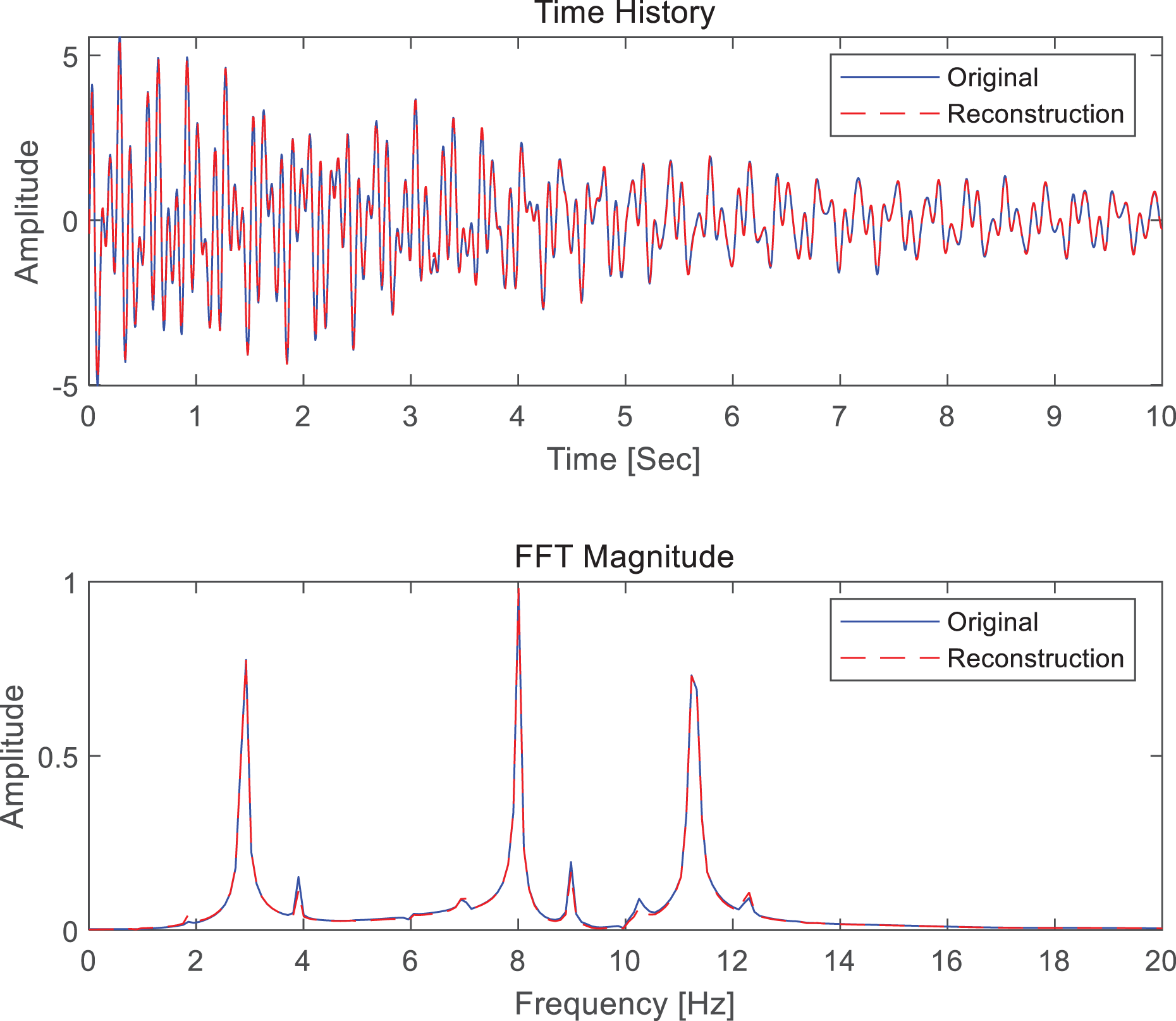
Time series and FFT magnitude of
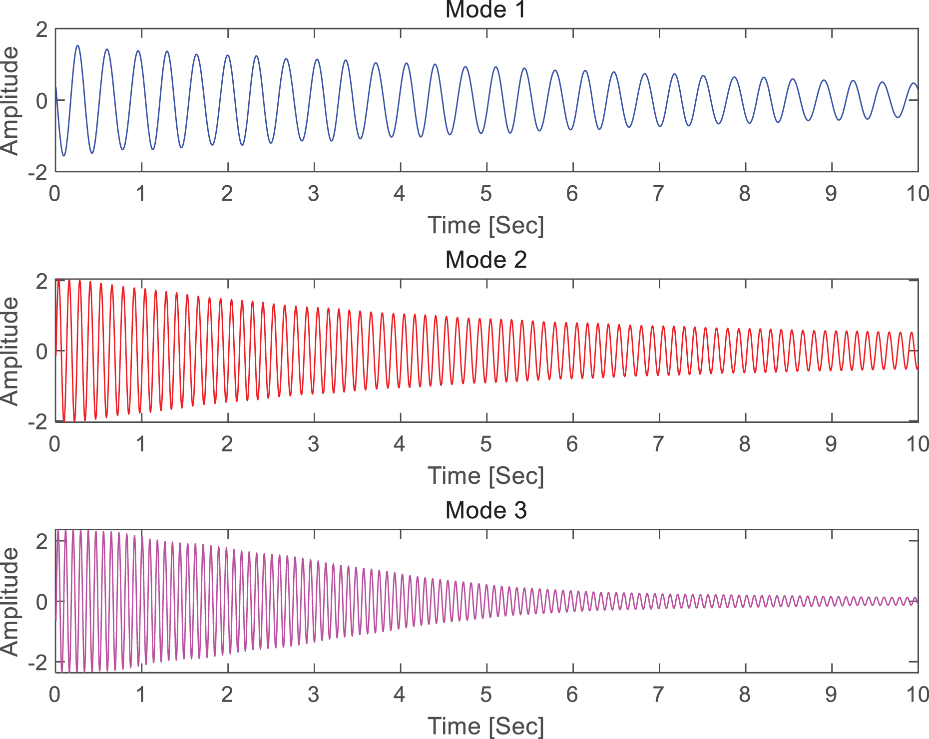
Monocomponents of the data
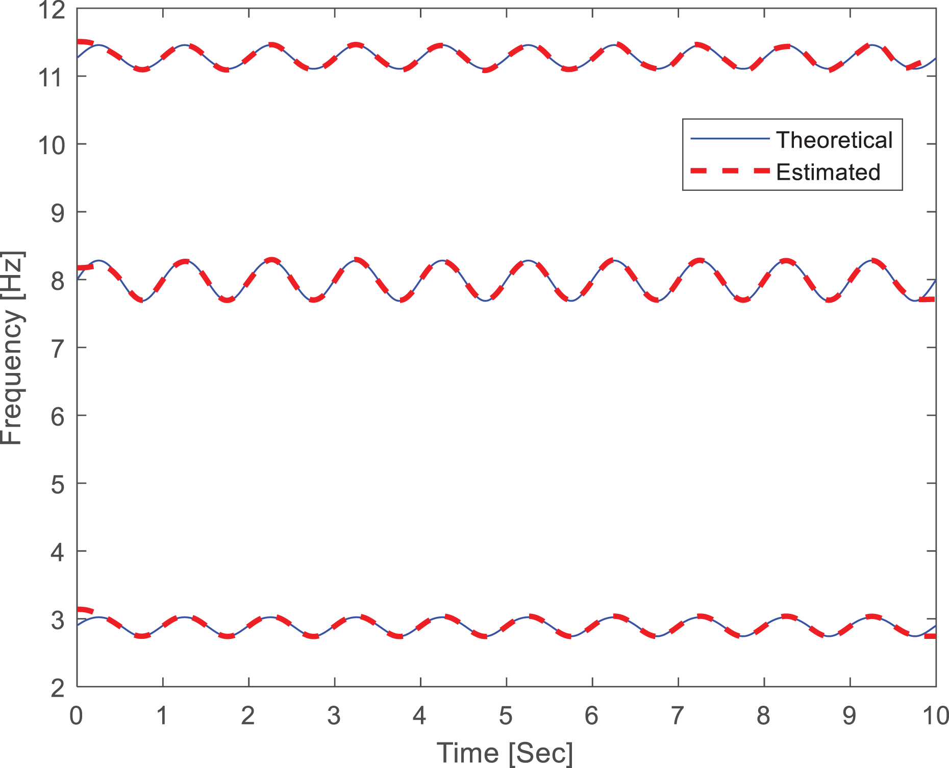
Instantaneous frequencies extracted by STNBMD and their theoretical values.
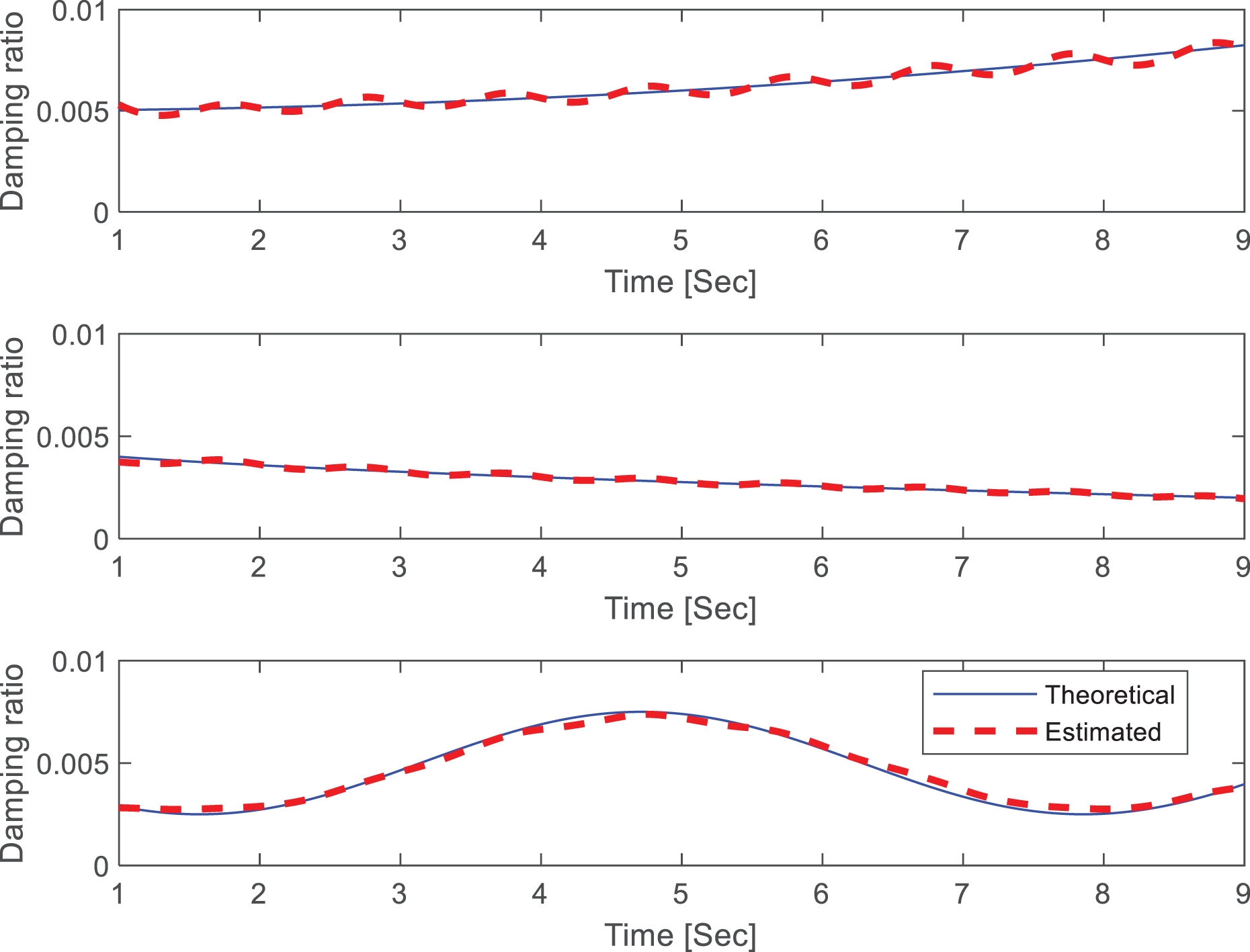
Damping ratios extracted by STNBMD and their theoretical values.
In addition, the mean absolute percentage error (MAPE) is utilized to evaluate the accuracy of the results, which is introduced by
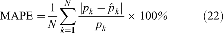
where pk
and
In this simulation, we obtain the MAPE of the natural frequencies is 0.26%, 0.09%, and 0.09% for mode 1, mode 2, and mode 3, respectively. The MAPE of the damping ratios is 3.27%, 2.51%, and 4.81% for mode 1, mode 2, and mode 3, respectively. These MAPEs are relatively small, and hence, the proposed method achieves ideal results in time-varying system identification.
Simple model of the Lysefjord bridge
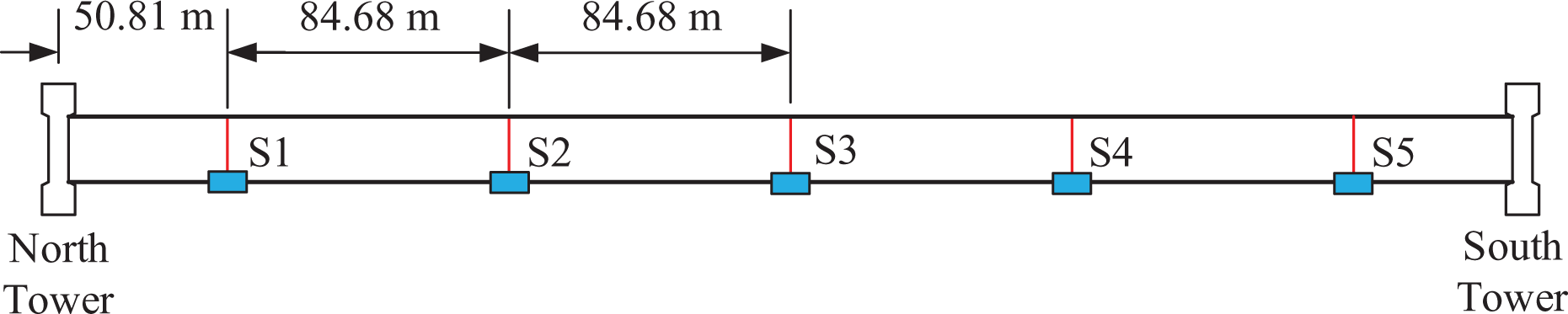
This numerical study is based on simulated displacement records of the Lysefjord bridge (Cheynet et al., 2016) using a simple model. The Lysefjord bridge, which is located in Rogaland, Norway, is a suspension bridge; its main span is 446 m. The displacement response has been calculated in five spots by Cheynet. These five locations along the span are numbered S1, S2,…, S5, as shown in Figure 9. The displacement response is recorded by a sampling frequency of 15 Hz, and a period of 3600 s is measured.
Five measured locations of the Lysefjord bridge (S4, S5 are symmetric to S1, S2).
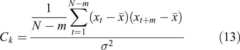
In this study, the displacement data in position S1 are employed for analysis. To better simulate the ambient vibration, the Gaussian noise of 10 dB is added to the analyzed data. Besides, a 2 Hz lowpass filter is applied for subsequent analyses. Figure 10 shows the time histories of the noisy data and its power spectra. Following the proposed approach, the ACF is employed to estimate the FVR of the displacement response of S1. Six frequencies, that is, 0.205, 0.317, 0.439, 0.583, 0.859, and 1.71 Hz, are obtained from the Fourier spectrum of the FVR. ESTNBMD is applied to the first 1500 samples of the FVR, and these six frequencies are employed as initial frequency values. The time history and Fourier spectrum of the original FVR and its reconstruction by ESTNBMD are displayed in Figure 11. The signal is adequately reconstructed. Figure 12 shows the extracted modes of the FVR using ESTNBMD owing to the end effect of HT; the estimated modes range from 10 to 95 s. In addition, curve fitting is applied to the extracted instantaneous frequencies; the results are shown in Figure 13. The damping ratios are calculated by equation (15) and they are listed in Table 2.
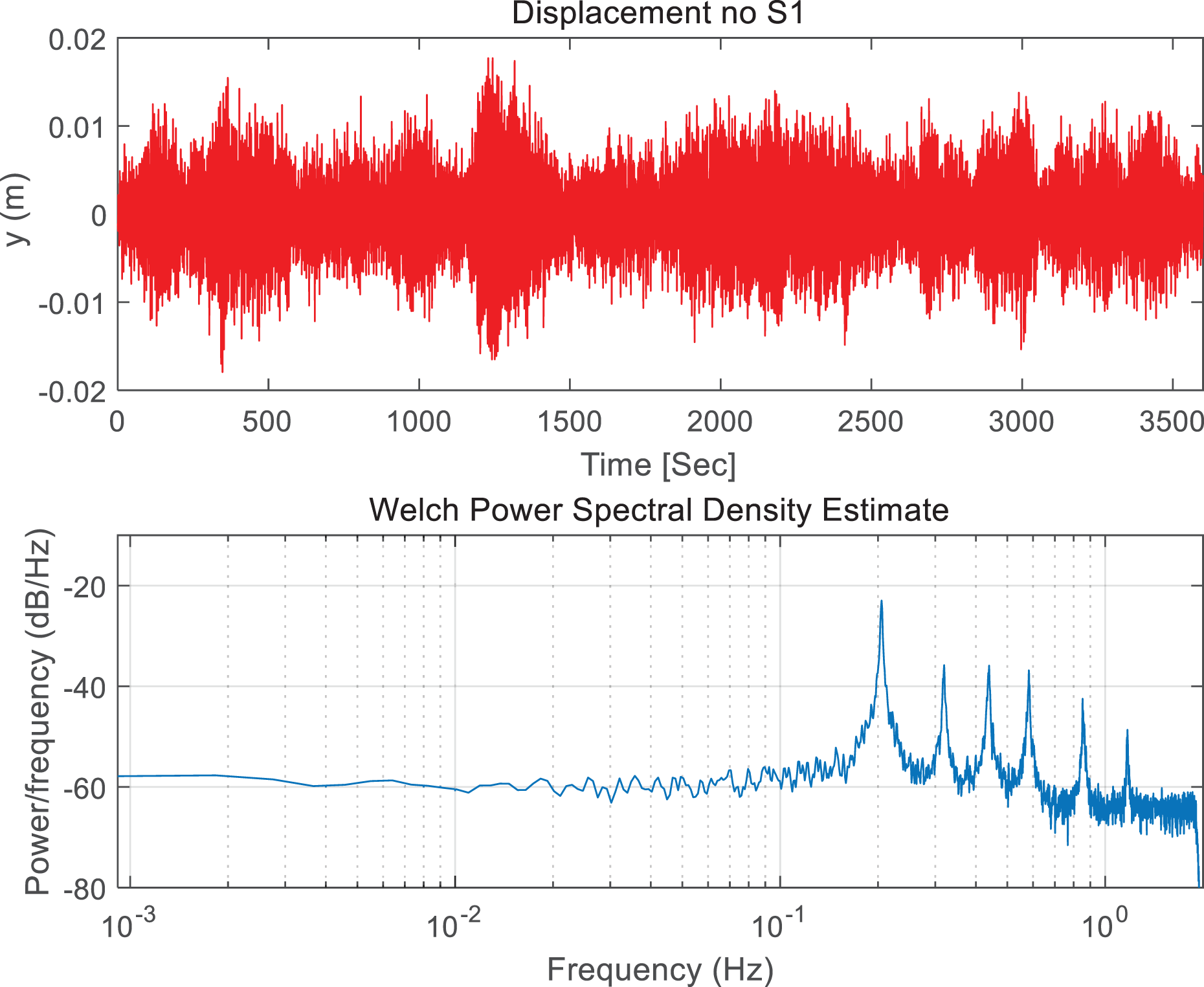
Time histories and power spectra of the displacement on S1.
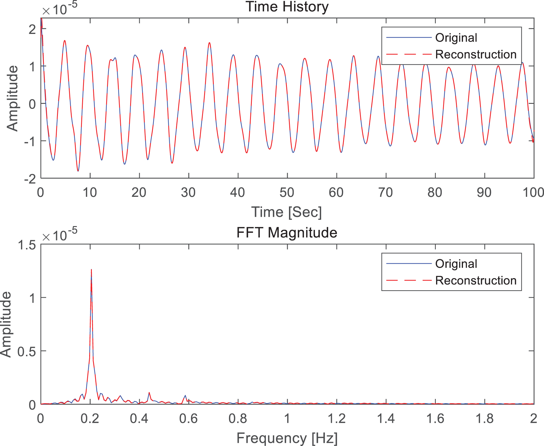
Magnitude of FVR and FFT of the displacement on S1: reconstruction compared with the original.
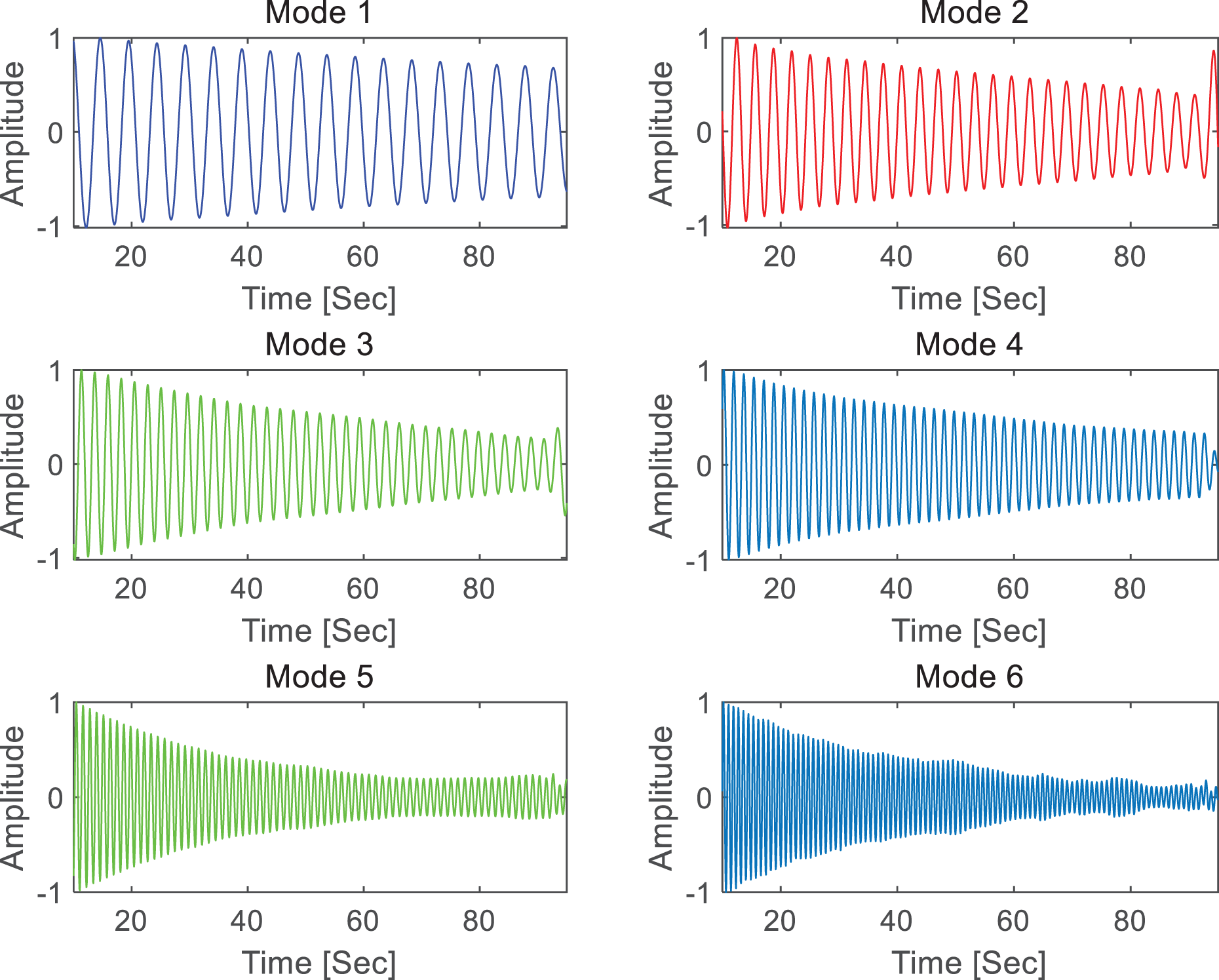
Monocomponents of the displacement on S1 estimated using ESTNBMD.
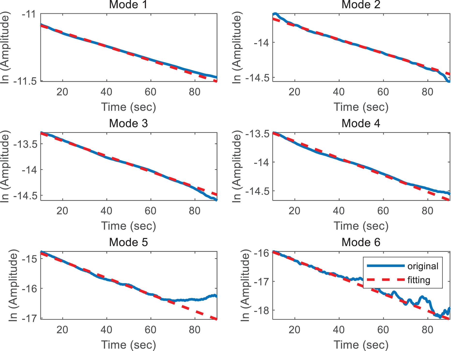
Instantaneous amplitudes extracted by ESTNBMD and their curve fitting results.
Comparison of the target values and the estimated natural frequencies and damping ratios.
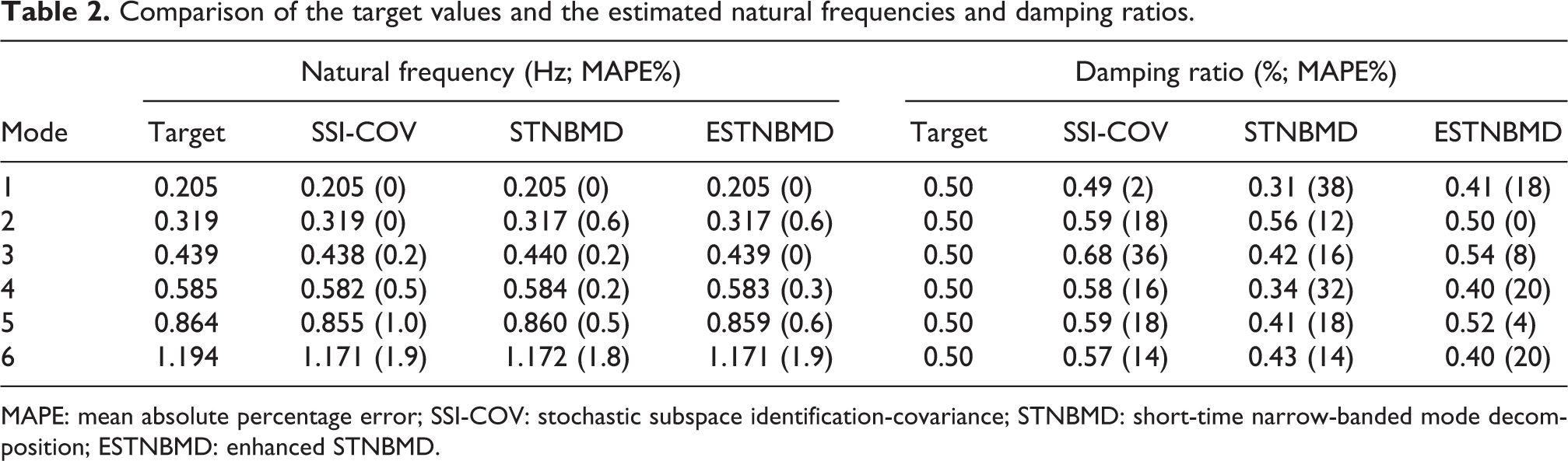
MAPE: mean absolute percentage error; SSI-COV: stochastic subspace identification-covariance; STNBMD: short-time narrow-banded mode decomposition; ESTNBMD: enhanced STNBMD.
For comparison with the results of the proposed method, a powerful MPI technique, that is, covariance-driven SSI (SSI-COV; Hermans and Van der Auweraer, 1999), and the primary STNBMD are employed in this example. Table 2 summarizes the natural frequencies and damping ratios gained by the proposed method, SSI-COV, and STNBMD, as well as the target value. The MAPEs are also provided.
The estimated natural frequency by ESTNBMD, SSI-COV, and STNBMD are similar to the target values. The highest MAPE of each method does not exceed 2%. However, these identified frequencies are more similar at higher frequencies and exhibit differences with the target values. This phenomenon is derived from the numerical scheme that is utilized for the time-domain simulation of the vibration response, which is dependent on the Newmark-β method. In the case of the damping ratios, these three approaches yield different results. The target values of the damping ratios are small, that is, 0.5%; hence, small discrepancies will yield a large MAPE. However, the highest MAPE of the proposed method is 20%, and that of SSI-COV and STNBMD is 36% and 38%, respectively. Moreover, the mean of the MAPE is 12%, 17%, and 22% for ESTNBMD, SSI-COV, and STNBMD, respectively. This feature shows that the proposed method outperforms the other two methods with regard to the damping ratios for the Lysefjord bridge.
Experimental study and validation
In this section, the proposed method is used to address the ambient vibration of the Dowling Hall footbridge, which is a two-span continuous steel truss bridge with a reinforced concrete deck located at Tufts University, United States (Figure 14(a)). The full length of the Dowling Hall footbridge is 44 m and the width is 3.9 m. From 5 January 2010 to 2 May 2010, 17 weeks were spent monitoring this footbridge. Eight accelerometers are installed in the Dowling Hall footbridge, that is, S1, S2,…, S8, and their locations are shown in Figure 14(b). In this monitoring experiment, a sampling frequency of 2084 Hz is adapted, and 300-s data samples are collected each hour. These data are processed by downsampling from 2084 to 128 Hz and applying a bandpass filter between 2 and 20 Hz for subsequent analyses. For more details about this project, refer to Behmanesh and Moaveni (2016) and Moaveni and Behmanesh (2012).
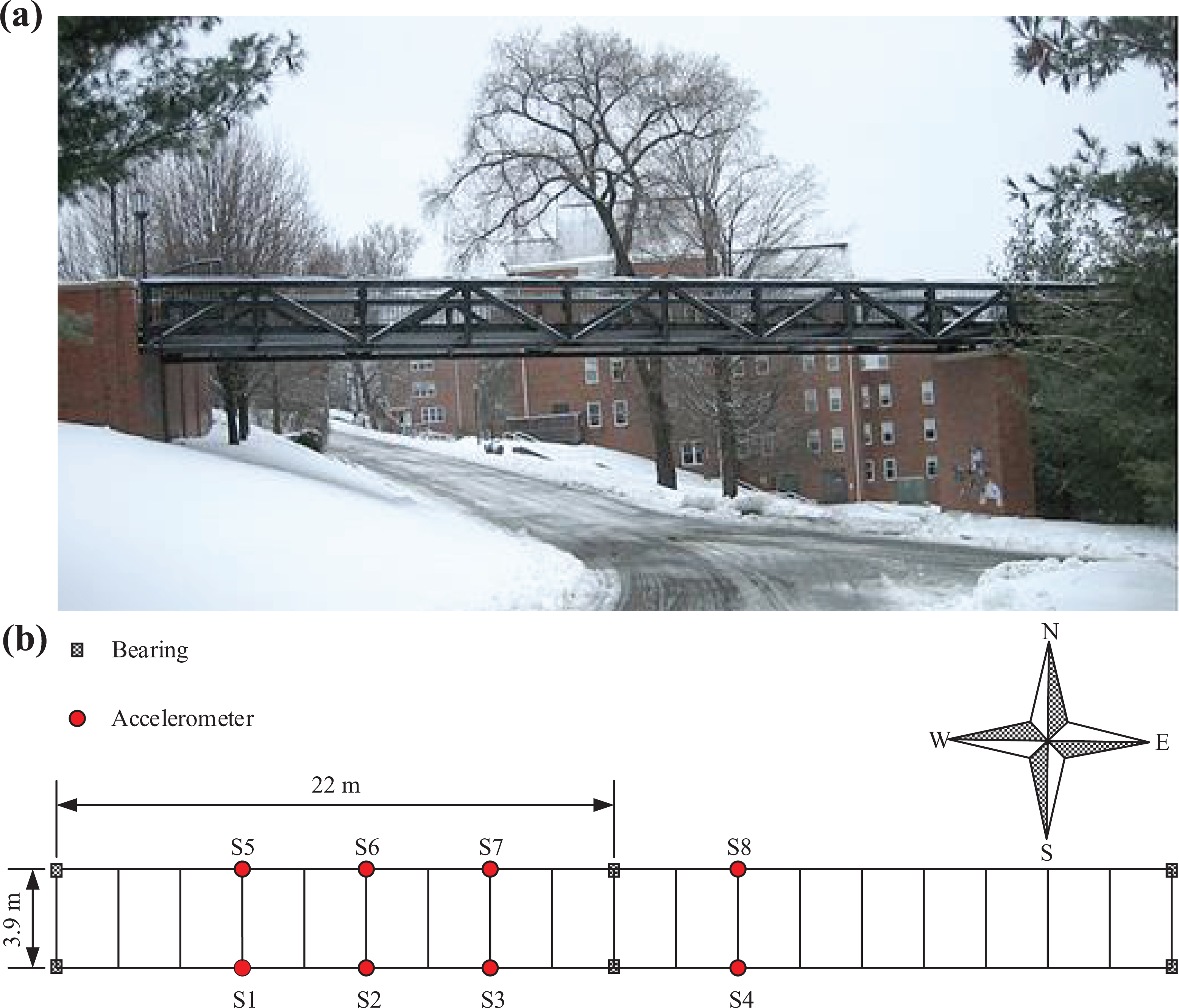
Dowling Hall footbridge and its sensor layout: (a) overview of the bridge and (b) sensor placement.
The measured data at 15:00 on 29 April 2010 are selected to verify the proposed method using a real-life structure in operational conditions. Only the acceleration data recorded by S3 are employed. The time history and power spectra of these data are shown in Figure 15.
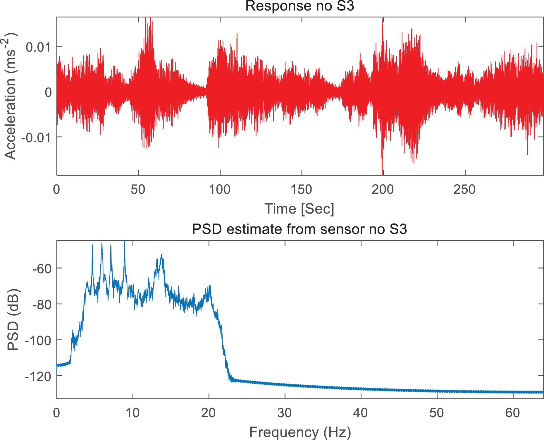
Time histories and power spectra of the acceleration on S3.
According to the new algorithm, the ambient vibration data obtained by S3 are converted to FVR using ACF. Using FFT to estimate the frequencies for the initial values of the instantaneous phases, the frequencies 4.67, 5.89, 7.11, 8.91, 13.20, and 13.75 Hz are obtained. The ESTNBMD method is applied to obtain the modes contained in the FVR. In this example, 1280 samples are selected for transformation, which corresponds to a duration of 10.0 s for the FVR signal. This chosen period is sufficient for extracting the FVR of the ambient vibration signal. After the instantaneous amplitudes are extracted, curve fitting is employed to calculate the damping ratios. All results are shown in Figures 16 to 18. The time series and Fourier spectrum of the extracted FVR and its reconstruction are obtained, as depicted in Figure 16, which reveals that the original FVR (solid line) and its reconstruction (dotted line) are similar, that is, ESTNBMD provides a high-precision reconstruction. Figure 17 shows the six modes estimated via the ESTNBMD approach, and the decay of mode 5 and mode 6 is fast. Hence, only the front parts of them are used for curve fitting. Figure 18 displays the results of the curve fitting of the instantaneous amplitudes. The natural frequencies and damping ratios identified by the proposed method are listed in Table 3.
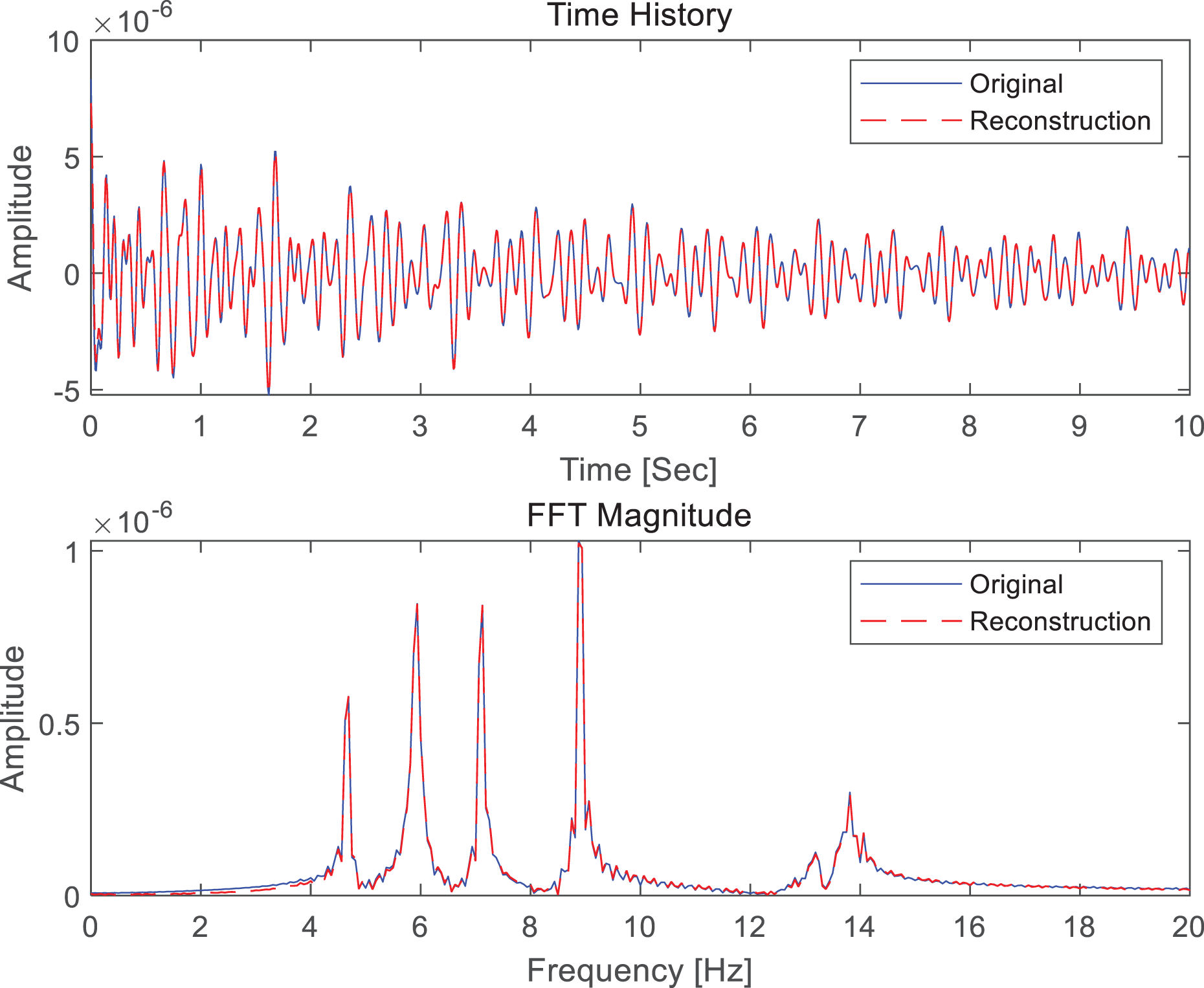
FVR and FFT magnitude of the data on S3: reconstruction compared with the original.
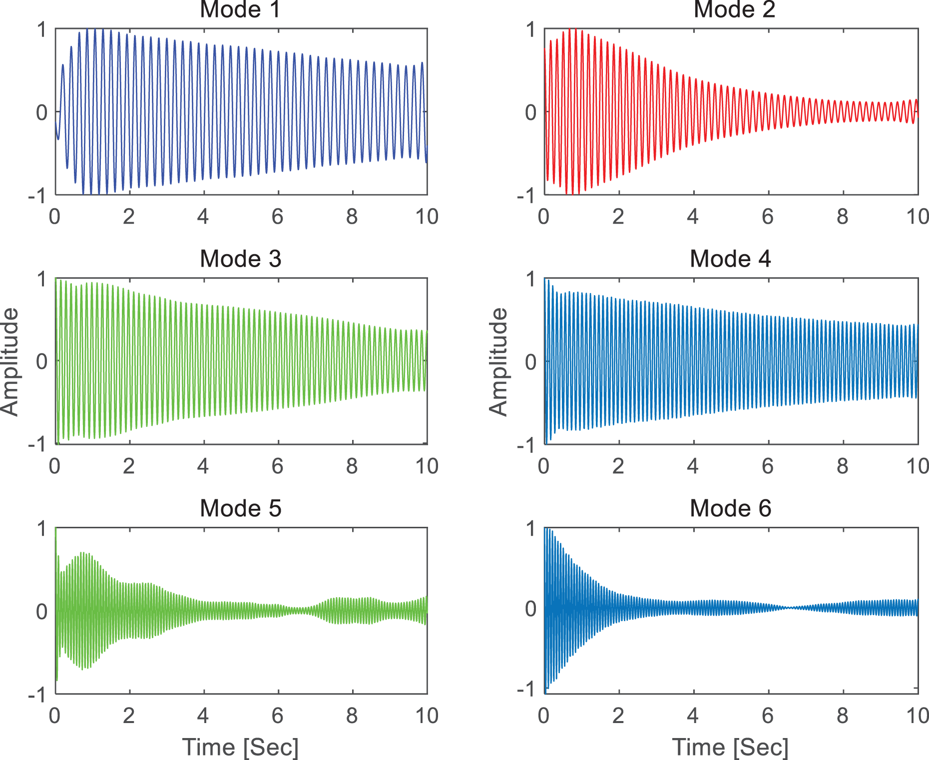
Monocomponents of the data on S3 estimated using ESTNBMD.
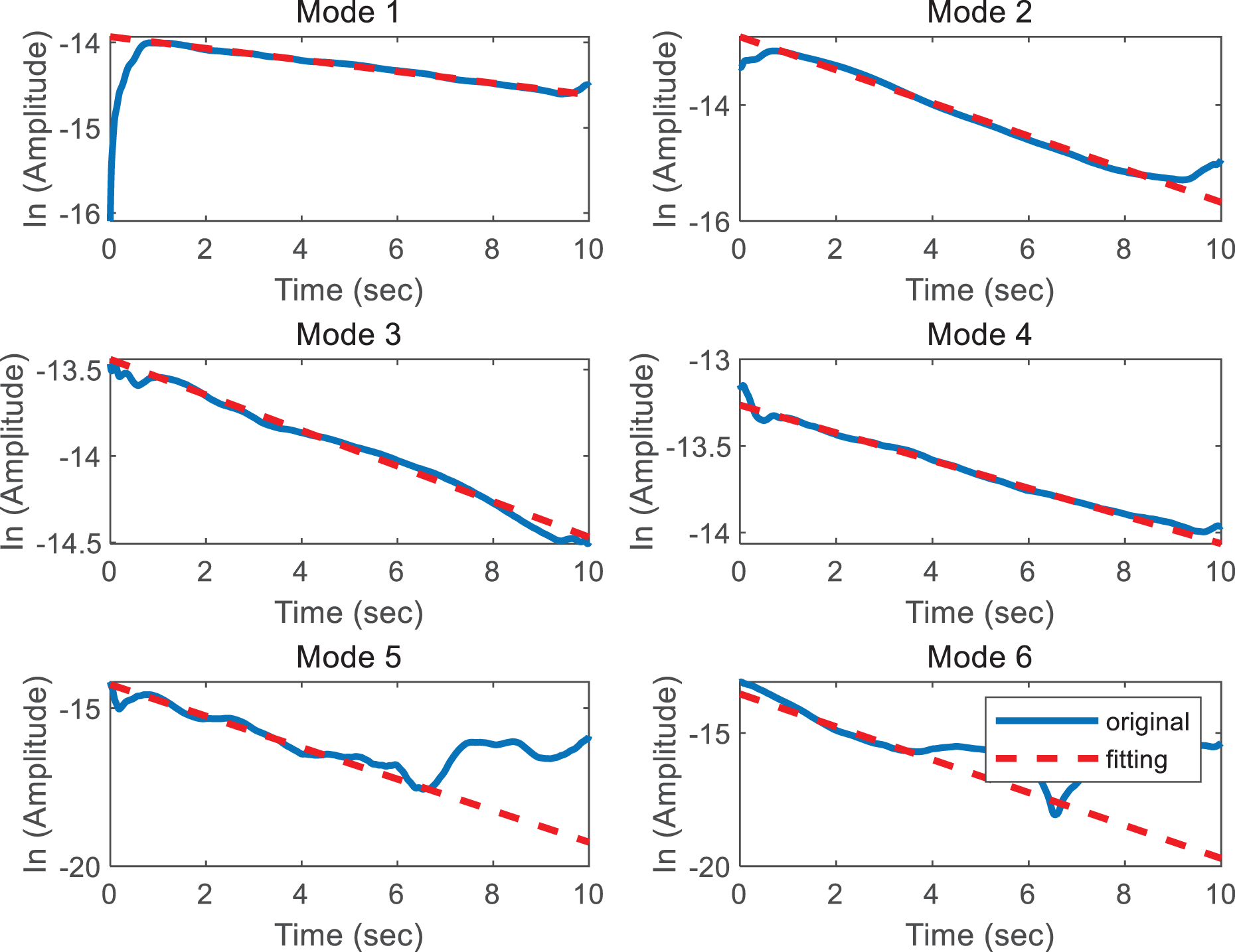
Instantaneous amplitudes extracted by ESTNBMD and their curve fitting results.
Estimated natural frequencies and damping ratios of the Dowling Hall footbridge.
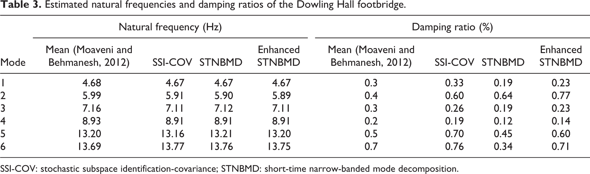
SSI-COV: stochastic subspace identification-covariance; STNBMD: short-time narrow-banded mode decomposition.
For comparison with the results obtained from the proposed approach, the SSI-COV algorithm and primitive STNBMD are applied. The results are also listed in Table 3. Except for the results acquired by the ESTNBMD, SSI-COV, and STNBMD, a previous study (Moaveni and Behmanesh, 2012) is also provided for comparison. However, unlike the results based on a 300-s period in this article, the reference values are the mean values during the monitoring period. Therefore, small discrepancies will exist between them and the extracted results.
Table 3 summarizes the reference values and the results of the ESTNBMD, SSI-COV, and STNBMD. The results reveal that the natural frequencies obtained by the three methods are identical to the frequencies in Moaveni and Behmanesh (2012). The natural frequencies identified by the proposed method are accurate. In general, the damping ratios identified by the proposed method and those of SSI-COV are similar to the mean in Moaveni and Behmanesh (2012), except for the second and fifth modes. Nevertheless, only the third and fifth modes of the damping ratio estimated by the STNBMD are similar to the mean. Hence, in this case, the results of ESTNBMD and SSI-COV outperform those of STNBMD regarding the damping ratios. These results demonstrate that the ESTNBMD method can identify the modal parameters of a real-life structure with satisfactory results, at least at the same level as SSI-COV and better than the primary STNBMD.
Concluding remarks
In this article, an MPI method with vibration signal decomposition was introduced. We exploit the STNBMD in the time-varying system with FVR and the ESTNBMD in time-invariant structures for MPI. Two numerical examples and an experimental study were employed to illustrate the efficiency of the proposed method.
The proposed approach can handle both ordinary structures and special structures with time-varying features. The results reveal that the proposed method has good performance in MPI. In addition, compared with the original STNBMD, the ESTNBMD approach has better performance and is less necessary for selecting parameters. This case satisfies the potential requirements of MPI.
In future work, the proposed method needs to be examined with additional field tests and numerical examples.
Footnotes
Authors’ Note
Baiben Chen is now affiliated with China Construction Third Engineering Bureau Co., Ltd, Wuhan, P.R. China.
Acknowledgements
The authors thank Prof. Fan Kong for critically reviewing the article.
Declaration of conflicting interests
The author(s) declared no potential conflicts of interest with respect to the research, authorship, and/or publication of this article.
Funding
The author(s) disclosed receipt of the following financial support for the research, authorship, and/or publication of this article: The authors received Nature Science Foundation of Hubei Province (2017CFB603) financial support for the research, authorship, and/or publication of this article.