A novel machine learning based tangent stiffness calculation method for 3D wheel-rail interaction element

Abstract

A machine learning (ML) based method is presented in this paper for obtaining tangent stiffness of a complicated three-dimensional wheel-rail interaction element that is able to practically and effectively simulate the complicated dynamic responses of vehicle-track problems. The element tangent stiffness, defined as differentiation of element insisting force to nodal displacement, is important in improving efficiency when Newton’s method is used to solve implicit nonlinear finite element equations. However, deriving and software implementing the tangent stiffness require significant efforts, and calculating the tangent stiffness in each iteration of the Newton method is usually time consuming. On the other hand, ML can directly obtain the implicit mapping between inputs and outputs of complex calculation process with limited programming effort and high computational efficiency, and is potentially a good alternative way to calculate the tangent stiffness of complicated element. In this paper, a feedforward artificial neural network is trained for obtaining the tangent stiffness, while inputs are the displacement and velocity of the element and outputs are the entries of the tangent stiffness matrix. The ML based tangent stiffness are implemented in an open source finite element software framework, OpenSees, and verified by application examples of a wheelset and a light rail vehicle running on straight rigid rail. The accuracy and efficiency are compared between the use of ML based tangent stiffness (MLTS) and the consistent tangent stiffness obtained at different speeds. The results demonstrate the MLTS can ensure the calculation accuracy and significantly improve the calculation efficiency.

Keywords

machine learning tangent stiffness wheel-rail interaction Newton’s method finite element method

Introduction

When an implicit method is used to discretize nonlinear finite element models with time, an iterative algorithm, for example, Newton’s method, can be used to solve the equations of motion at each time step. In this case, the element tangent stiffness, defined as the differentiation of element insisting force to nodal displacement, plays a crucial role in improving computational efficiency. The so-called consistent tangent stiffness (Simo JC and Taylor RL, 1985; Miehe C, 1996; Doghri I, 1993) is accurate and guarantees a quadratic rate of convergence of Newton’s method. Planinc and Saje (1999) presented a quadratically convergent algorithm for the computation in the finite element formulation by linearizing the determinant of the global tangent stiffness matrix, and prove the advantage of large convergence radius. Gu et al. (2011) presented consistent tangent moduli for a pressure independent multi-yield-surface J2 (Von Mises) plasticity model and investigated the convergence rate and computational time. Jirasek and Patzak (2002) presented a general framework for a consistent derivation of the “nonlocal” tangent stiffness, demonstrated the quadratic rate of convergence of the Newton–Raphson iteration procedure. The derivation and software implementation of the consistent tangent stiffness usually requires significant efforts. Therefore, it is desirable to develop an alternative method to compute the tangent stiffness that can maintain high computational efficiency while reduce the efforts of derivation and software implementation.

Dynamic response analysis of high-speed railway is usually large-scale, highly nonlinear and requires significant computational effort, among which the calculation of wheel-rail interaction (WRI) forces is one of the most time-consuming parts. Many wheel-rail contact models have been proposed for addressing WRI problems. Zhai et al. (1996, 2009), Zhai (2004) and Chen and Zhai (2004) used a fast explicit integration method to solve the motion equations and then calculated WRI forces by using a vehicle-track coupling model. Dinh et al. (2009) developed a formulation for the 3D dynamic interactions between a bridge and a high-speed train. Pombo et al. (2007) presented a wheel-rail contact detection formulation and calculated the tangential forces by using Kalker’s linear theory, Heuristic nonlinear model, and Polach formulation. Then Magalhaes et al. (2020) and Marques F et al. (2020, 2019) extended the online Hertzian contact model proposed by Pombo to propose a non-Hertzian contact model. Gu et al. (2019) presented a 2D WRI element consisting of a fast-moving wheel node and rail nodes that the wheel node may pass through. The WRI force is wrapped into the element as the elemental resisting force. Liu et al. (2021) developed a three-dimensional (3D) WRI element based on the same idea wrapping the WRI into a 3D element, the WRI force of which is obtained by using Kalker’s linear theory, nonlinear Hertz theory, and Polach formulation. The consistent tangent stiffness (Gu Q et al., 2021) of the 3D WRI element is derived, the accuracy and the efficiency of the algorithm are compared with the perturbation method (Liu et al., 2021) and the quadratic convergence rate is proved.

Recently, machine learning (ML) has been increasingly widely applied in engineering to solve a wide range of problems. ML can directly obtain the implicit mapping between inputs and outputs of complex calculations with relatively little formula derivation and programming work. ML can potentially be used to solve complex nonlinear problems simply and efficiently (Jung and Ghaboussi, 2006; Luo and Paal, 2018; Huang and Loh, 2001; Kang et al., 1997). Li and He (2015) presented an algorithm, that is, Random Forests-based nonparametric missing value imputation algorithm, to predict remaining useful life (RUL) of wheels and trucks (bogies), where the missing data are handled by missForest. Wang et al. (2019) proposed a bilevel superpixel-based framework for the vision inspection of rail conditions and automatically detected rail surface cracks. Mohammadi et al. (2019) developed a new ML based approach to identify the track geometry parameters employing an extreme gradient boosting algorithm, in which the hyper-parameters are optimized using a Bayesian optimization method. Acikbas and Soylemez (2008) combined ANN and genetic algorithms to achieve optimal coasting points for long line sections that cover five stations and two lines. The ML approach has demonstrated high accuracy and efficiency in the above various applications. However, ML has not yet been applied to solve tangent stiffness of complex nonlinear systems, for example, WRI system.

In this paper, an ML based tangent stiffness (MLTS) method is applied to a WRI element proposed by Liu et al. (2021). A feedforward artificial neural network (ANN) using error back-propagation (BP) training is used to obtain the tangent stiffness, where the input is displacement and velocity of the element and output is the tangent stiffness matrix. The tangent stiffness used for training ANN is obtained by perturbation method. The trained ANN model is implemented in an open source finite element software, OpenSees. The responses of the WRI element using ML based tangent stiffness (MLTS) and the traditional consistent tangent stiffness (CTS) (Gu et al., 2021) are compared to verify the accuracy and efficiency of MLTS. The proposed ML based tangent stiffness calculation method herein has the following advantages: (1) the efforts of derivation and software implementation of the ANN model are relatively small, (2) the computation is efficient with acceptable accuracy, and (3) the method is applicable under different working conditions, for example, vehicles with multiple wheelsets and running at different speeds. There are some limitation of the proposed method: (1) obtaining the samples and training ANN model require time and efforts, (2) programming the ANN model requires efforts, although usually much smaller than CTS, and (3) the Newton quadratic convergence cannot be guaranteed when solving the nonlinear equation of motion. A future research direction could be optimizing the algorithm and applying the MLTS calculation method to a wide range of realistic problems that require tangent stiffness, for example, complicated vehicle–track–bridge systems. Besides, the method may be useful in performance assessment of complicated systems based on Monte Carlo simulation or reliability analysis.

Tangent stiffness calculation

Equilibrium equation of motion and the consistent tangent stiffness

In the numerical modeling of the civil engineering structures, a specific element is often implemented in a finite element (FE) software framework, for example, OpenSees in this paper, which allows combining the element with the abundant material library available in it. The equilibrium equation of motion of the element is same as that in an FE method

M \ddot{u} (t) + C \dot{u} (t) + R (u (t)) = F (t)

(1)

where M denotes mass matrix, C denotes damping matrix, R is the resisting force of the element, and F is the element’s load vector.

\ddot{u}

\dot{u}

, and u are the acceleration, velocity, and displacement of the element, respectively. The Newmark-β method is used to replace the time-stepping discretization scheme in equation (1).

\ddot{u}

and

\dot{u}

are calculated as

{\dot{u}}_{n + 1} = (Δ t) (1 - \frac{α}{2 β}) {\ddot{u}}_{n} + (1 - \frac{α}{β}) {\dot{u}}_{n} + \frac{α}{(Δ t) β} (u_{n + 1} - u_{n})

{\ddot{u}}_{n + 1} = (1 - \frac{1}{2 β}) {\ddot{u}}_{n} - \frac{1}{(Δ t) β} {\dot{u}}_{n} + \frac{1}{{(Δ t)}^{2} β} (u_{n + 1} - u_{n})

(2)

where α and β are Newmark parameters and Δt is the time increment. The subscripts n and n+1 represent the previous times step n and current time step n+1, respectively. Substituting equation (2) into equation (1) yields the residual of unbalanced force that is the same as in FE

Ψ (u_{n + 1}) = {\bar{F}}_{n + 1} - [(\frac{1}{{(Δ t)}^{2} β} M + \frac{α}{(Δ t) β} C) u_{n + 1} + R (u_{n + 1})] = 0

{\bar{F}}_{n + 1} = F_{n + 1} + M [\frac{1}{{(Δ t)}^{2} β} u_{n} + \frac{1}{(Δ t) β} {\dot{u}}_{n} - (1 - \frac{1}{2 β}) {\ddot{u}}_{n}] + C [\frac{α}{(Δ t) β} u_{n} - (1 - \frac{α}{β}) {\dot{u}}_{n} - Δ t (1 - \frac{α}{2 β}) {\ddot{u}}_{n}]

(3)

where

Ψ (u_{n + 1})

denotes residual unbalanced force, which may be solved iteratively using a root-finding algorithm, for example, the Newton iteration method, whose updating rule is

u_{n + 1}^{i + 1} = u_{n + 1}^{i} - Ψ^{'} {(u_{n + 1}^{i})}^{- 1} \cdot Ψ (u_{n + 1}^{i}) (i = 1,2,3...)

(4)

where the superscript denotes the number of iterations. Equation (4) will be performed for each iteration until

| Ψ (u_{n + 1}) | < t o l

(5)

is satisfied, where tol denotes a given tolerance. In equation (4),

Ψ^{'} (u_{n + 1}^{i})

denotes the derivative of

Ψ (u_{n + 1}^{i})

with respect to u_n+1 in i^th iteration. The process of newton method is shown in Figure 1 for solving nonlinear equilibrium equation of motion.

Figure 1.

Process of Newton method.

The blue line denotes the change of $Ψ (u_{n + 1})$ with nodal displacement $u$ . Each red line denotes one Newton iteration to obtain an approximate solution $u$ . After three iterations $| Ψ_{n + 1} |$ is less than a specified tolerance and the iterative process stops. The slope of the red line $(Ψ^{'} (u))$ is defined as tangent stiffness (CTS) of the element that plays an important role in guaranteeing a quadratic convergence rate of Newton iteration. $Ψ^{'} (u)$ can be expressed as

Ψ^{'} (u) = \frac{\partial Ψ (u)}{\partial u} = - \frac{\partial R (u)}{\partial u}

(6)

Generally, since the calculation of CTS requires a lot of efforts and is time-consuming, it is desirable to develop an ANN based tangent stiffness that can maintain high computational efficiency while reduce the efforts of derivation and software implementation.

Internal resisting force and the CTS of the WRI element

As shown in Figure 2, the WRI element consists of a wheel node and all the rail nodes (b₁, b₂ … b_i …) that the wheel node may pass through. The wheel node and the adjacent rail node are combined into a so-called active portion (red wireframe in Figure 2), and all node resisting force in active portion can be regarded as the resisting force R (see equation (1)), which is represented by black arrows in zoomed view of Figure 2. It is clear R consists of 18 components. R can be obtained by

R = f (F^{c})

(7)

where F^c denotes the contact force between wheel and rail and

f

represents the function (Liu et al., 2021) related to coordinate system transformation and virtual work principle. Furthermore, F^c consists of three parts

F^{c} = {\begin{cases} F_{n}^{c} \\ F_{t x}^{c} \\ F_{t y}^{c} \end{cases}}

(8)

where

F_{n}^{c}

denotes normal contact force and

F_{t x}^{c}

and

F_{t y}^{c}

are the tangential contact force in the longitudinal and lateral directions (Figure 2). The normal contact force

F_{n}^{c}

is calculated through the following steps: 1) represent the wheel and rail profiles with piecewise linear curves, search and determine the contact point, 2) calculate the maximum virtual interpenetration depth of the wheel and rail profiles, and 3) calculate the normal force

F_{n}^{c}

by applying nonlinear Hertz theory (Hertz H, 1882)

F_{n}^{c} = k_{h} {(δ_{\max})}^{1.5}

(9)

where

δ_{\max}

denotes the maximum virtual interpenetration depth,

k_{h}

denotes the generalized stiffness coefficient, which is depends on the Young modulus and the Poisson ratio, and on the curvatures of the surfaces at the contact point and so on (Shabana A et al., 2008). The tangential contact force are determined by applying Polach formula (Polach O, 1999), as shown in equation (10). Detailed formulas can be referred to literature (Liu Y et al., 2021).

{\begin{cases} F_{t x}^{c} = F_{t r} \frac{S_{x}}{S_{c}} \\ F_{t y}^{c} = \frac{1}{S_{c}} (F_{t r} S_{y} + F_{y s} ψ) \end{cases}

(10)

where

S_{x}

denotes the translational creep in the X coordinate direction,

S_{y}

denotes the translational creep in the Y coordinate direction, and

ψ

is the spin creep.

S_{c}

represents modified translational creepage.

F_{tr}^{c}

is a resultant tangential force and

F_{ys}^{c}

represents the lateral tangential force caused by pure spin.

Figure 2.

WRI element and its resisting force R

The consistent tangent stiffness (CTS) of the WRI element can be obtained by differentiating each equation mentioned in Internal resisting force and the CTS of the WRI element (i.e., equations (7)–(10)) with respect to u by the chain rule, that is,

\frac{\partial R}{\partial u} = \frac{\partial f (F^{c})}{\partial F^{c}} \cdot \frac{\partial F^{c}}{\partial u}

(11)

The detailed derivation of $\partial F^{c} / \partial u$ can be found in literature (Gu et al., 2021). R and u are both vectors with 18 entries, so $\partial R / \partial u$ can be assembled into a so-called tangent stiffness matrix with a size of 18 $\times$ 18

\frac{\partial R_{m}}{\partial u_{n}} = [\begin{matrix} \frac{\partial R_{1}}{\partial u_{1}} & \dots & \frac{\partial R_{18}}{\partial u_{1}} \\ ⋮ & ⋱ & ⋮ \\ \frac{\partial R_{1}}{\partial u_{18}} & \dots & \frac{\partial R_{18}}{\partial u_{18}} \end{matrix}] = [\begin{matrix} T_{1,1} & \dots & T_{18,1} \\ ⋮ & ⋱ & ⋮ \\ T_{1,18} & \dots & T_{18,18} \end{matrix}]

(12)

The machine learning model

Feedforward ANN model

An artificial neural network (ANN) using error back-propagation (BP) algorithm is used to obtain the tangent stiffness in this paper. The ANN model has an input layer, a hidden layer, and an output layer (Figure 3). Each layer is made up of a few neurons. The number of neurons in input and output layers is usually determined by number of input parameters and output parameters, while the number of neurons in the hidden layer is uncertain. Too few neurons may affect the accuracy of the predicted results, but too many may lead to overfitting. Therefore, multiple tests are often needed to select the best number of hidden layer neurons.

Figure 3.

A representation of the feedforward ANN.

In the hidden layer, each neuron receives parameters from the input layer and then calculates as follows

h_{i} = f (\sum_{j = 1}^{m} w_{i j} X_{j} + b_{i}), i = 1, ..., n

(13)

where n denotes the number of neurons in the hidden layer and m denotes the number of inputs. h_i denotes the i^th neuron of the hidden layer and i ranges from 1 to n. X_j is the j^th input, where j ranges from 1 to m. w_ij is a weighting coefficient for X_j’s contribution to

h_{i}

, while

b_{i}

is a bias for the i^th neuron in the hidden layer. f represents a nonlinear activation function, which builds the nonlinear mappings. There are many forms for f, but in this study the tanh function was used, which expressed as

f (x) = \frac{e^{x} - e^{- x}}{e^{x} + e^{- x}}

(14)

where e denotes the basis of the natural logarithms. After each neuron in the hidden layer has been calculated, the neurons in output layer can be expressed as

Y_{j} = \sum_{i = 1}^{N} v_{j i} h_{i} + d_{j}, j = 1, ..., M

(15)

where M denotes the number of outputs and N is the number of neurons in the hidden layer.

Y_{j}

represents the j^th output, where j ranges from 1 to M. h_i is the i^th neuron of the hidden layer, i ranges from 1 to n. v_ji is a weighting coefficient for the contribution of h_i to

Y_{j}

, while d_j denotes the bias for the j^th output. The weighting coefficients and biases (w_ij, b_i, v_ji, and d_j) in equations (13) and (15) can be obtained by reducing the total error of the network through continuously adjusting the weighting coefficients and biases (w_ij, b_i, v_ji, and d_j). The total error of the ANN is defined as

E = \frac{1}{2} {\sum_{j = 1}^{M} ({\hat{Y}}_{j} - Y_{j})}^{2}

(16)

where

Y_{j}

denotes the output calculated by equation (15) and

{\hat{Y}}_{j}

denotes the expected output of the j^th output layer neuron. A gradient descent method (Mordecai A, 2003) is used to reduce the total error of the network by continuously adjusting the weighting coefficients and biases (w_ij, b_i, v_ji, and d_j). Taking v_ji as an example, the gradient is

Δ ν_{j i} = - η \frac{\partial E}{\partial ν_{j i}}

(17)

where

η

is the learning rate of BP neural network (0.0001 in this paper).

\partial E / \partial ν_{j k}

can be obtained by

\frac{\partial E}{\partial ν_{j i}} = \frac{\partial E}{\partial E_{j}} \cdot \frac{\partial E_{j}}{\partial Y_{j}} \cdot \frac{\partial Y_{j}}{\partial v_{j i}}

(18)

According to equation (15) and (16)

\begin{array}{l} \frac{\partial E}{\partial E_{j}} = \sum_{j = 1}^{M} ({\hat{Y}}_{j} - Y_{j}) \\ \frac{\partial E_{j}}{\partial Y_{j}} = - 1 \\ \frac{\partial Y_{j}}{\partial ν_{j i}} = h_{i} \end{array}

(19)

The updating rule (i.e., adjustment) of

Δ ν_{j i}

, d_j, w_ij, and b_i are

Δ ν_{j i} = η \sum_{j = 1}^{M} ({\hat{Y}}_{j} - Y_{j}) h_{i}

(20)

\begin{array}{l} Δ d_{j} = η \sum_{j = 1}^{M} ({\hat{Y}}_{j} - Y_{j}) \\ Δ ω_{i j} = η \sum_{j = 1}^{M} ({\hat{Y}}_{j} - Y_{j}) ν_{j i} f^{'} (h_{i}) X_{j} \\ Δ ω_{i} = η \sum_{j = 1}^{M} ({\hat{Y}}_{j} - Y_{j}) ν_{j i} f^{'} (h_{i}) \end{array}

(21)

After this adjustment, re-evaluating equation (16) to check whether the error is less than a specified criterion, and if not, repeating equations (16)–(21) until the tolerance requirement is satisfied.

Since ANN is only one of the machine learning (ML) models, it is necessary to apply other machine learning methods for prediction and compare the advantages and disadvantages of different ML methods. A nonlinear autoregressive model with exogenous inputs (NARX) model is used for this purpose.

Nonlinear autoregressive models with exogenous inputs (NARX) model

An NARX is used to obtain the tangent stiffness and compare it with that obtained by ANN. NARX is a class of discrete-time nonlinear systems that can be mathematically represented as

Y (n) = f_{N} [\hat{Y} (n), ..., \hat{Y} (n - d_{y} + 1); X (n), X (n - 1), ..., X (n - d_{x} + 1)]

(22)

where X and Y denote input and output of the model at discrete time step n, respectively. d_x and d_y are the input-memory and output-memory orders.

\hat{Y}

denotes the actual output, using which (instead of using

Y

, see Figure 4) can reduce cumulative error. f_N denotes the implicit mapping from the input to the output.

Figure 4.

Implicit mapping of the NARX.

The TDLF in Figure 4 denotes the tapped delay line filter, which can be expressed as

\begin{array}{l} X_{n} (n) \to X_{n} (n), X_{n} (n - 1), ... X_{n} (n - d_{x} + 1) \\ {\hat{Y}}_{m} (n) \to {\hat{Y}}_{m} (n), {\hat{Y}}_{m} (n - 1), ..., {\hat{Y}}_{m} (n - d_{y} + 1) \end{array}

(23)

The values of d_x and d_y are set as 2. After the input of NARX is filtered by TDLF, the resulting network has a purely feedforward architecture, and static back-propagation can be used for training (see equations (13)–(21)). Considering that the NARX is more time-consuming than ANN, the neurons of the hidden layer is reduced to 10 after tests by authors.

Comparison of two ML models

The performances of the two models are compared based on their predicted results. A mean squared error (MSE) of the discrepancies is defined as

MSE= \frac{{\sum_{j=1}^{R} ({\hat{Y}}_{j} - Y_{j})}^{2}}{R}

(24)

where R denotes the size of sample.

\hat{Y}

denotes the actual output while

Y

denotes the estimated output. Another indicator, that is, coefficient of determination R², is defined as

\begin{array}{l} R^{2} = 1 - \frac{S S_{res}}{S S_{tot}} \\ S S_{res} = {\sum_{i} ({\hat{Y}}_{i} - Y_{i})}^{2} \\ S S_{tot} = {\sum_{i} (Y_{i} - {\bar{Y}}_{i})}^{2} \end{array}

(25)

where

{\bar{Y}}_{j}

denotes the average value of the sample. The closer R² is to 1, the better the performance of the model is. Table 1 compares MSE and R² between the actual output and the estimated output obtained by the two models (taking T_1,1 and T_2,2 as an example) based on the sample mentioned in Data of ML based tangent stiffness in a wheelset example. The results show that ANN model is notably better than NARX in the sense of both accuracy and efficiency in this case. Therefore, ANN model is used in the following paper.

Table 1.

Comparison of two models.

Entries of tangent stiffness matrix	The ML model	MSE	R ²	Training time (min)
T_1,1	ANN	0.0011	0.9048	75
T_1,1	NARX	0.0158	0.8770	124
T_2,2	ANN	0.0027	0.8790	75
T_2,2	NARX	0.0042	0.8254	124

Application examples

Data of ML based tangent stiffness in a wheelset example

A previously-studied wheelset example (Pombo J, 2004) is used to get samples of ANN. As can be found in Figure 2, a single wheelset is running on a straight rigid rail. Before the dynamic analysis of the wheelset, a horizontal force is applied in lateral direction such that an original misalignment of the wheelset is 2 mm. The wheel and rail profiles used are the UIC50 and ML95 (Pombo J and Ambrosio J, 2005). More details of the model can be found in the literature (Liu Y et al., 2021; Pombo J, 2004). The Newmark-Beta method is used for the time integration with $γ=0 .5$ and $β=0 .25$ with a time step of 0.001 s. The speed assumed in this example to be 20 m/s.

The displacement and velocity (u and

\dot{u}

) play a fundamental role in determining the geometric positioning and calculating the resisting force of the WRI element, as well as the tangent stiffness. u and

\dot{u}

can be regarded as inputs to ANN. Since the rail is rigid, the degrees of freedom of all the rail nodes are fixed, so the only inputs are the displacement and velocity of the wheel node (

u^{w}

and

{\dot{u}}^{w}

) and the number of inputs is 12. As for the output, 324 entries in the tangent stiffness matrix (equation (12)) are divided into 18 groups (column vectors of the stiffness matrix) and predicted independently in order to improve efficiency. The model is run for 10,000 time steps, and it takes an average of 6 iterations in each time steps. Then, a total of 61,206 input and output samples were obtained. Evaluating the neural network’s efficiency and accuracy suggested that a neural network with one hidden layer of 20 hidden layer neurons is optimal. The ANN is trained according to equations (13)–(21) to obtain the machine learning based tangent stiffness (MLTS). 10-fold cross-validation (Dietterich T, 1998) is used to test whether there is overfitting. The sample is divided into 10 sub samples, in which one sub sample (test set) is retained as the data to validating model, and the other 9 samples (training set) are used for training purpose. Three components in the tangent stiffness matrix are used to evaluate the results, that is, T_1,1, T_1,2, and T_1,3 (equation (12)). The process is repeated 10 times for each component and the coefficient of determination R² for trained and tested data are shown in the Table 2. The average results of R² are listed in the table as well. It is observed that the R² of test set is slightly lower than that of the training set, indicating that the overfitting of the model in this paper is within the acceptable range. The calculating process of MLTS can be found in Figure 5.

Table 2.

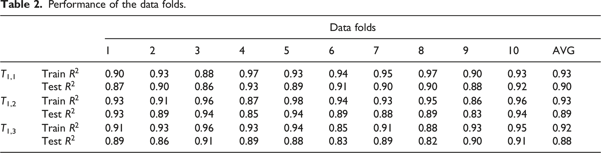
Performance of the data folds.

		Data folds
		1	2	3	4	5	6	7	8	9	10	AVG
T _1,1	Train $R^{2}$	0.90	0.93	0.88	0.97	0.93	0.94	0.95	0.97	0.90	0.93	0.93
T _1,1	Test $R^{2}$	0.87	0.90	0.86	0.93	0.89	0.91	0.90	0.90	0.88	0.92	0.90
T _1,2	Train $R^{2}$	0.93	0.91	0.96	0.87	0.98	0.94	0.93	0.95	0.86	0.96	0.93
T _1,2	Test $R^{2}$	0.93	0.89	0.94	0.85	0.94	0.89	0.88	0.89	0.83	0.94	0.89
T _1,3	Train $R^{2}$	0.91	0.93	0.96	0.93	0.94	0.85	0.91	0.88	0.93	0.95	0.92
T _1,3	Test $R^{2}$	0.89	0.86	0.91	0.89	0.88	0.83	0.89	0.82	0.90	0.91	0.88

Figure 5.

Calculating process of MLTS.

Verify the ML based tangent stiffness at various velocities

The same example in Data of ML based tangent stiffness in a wheelset example is used to verify the MLTS herein. Lateral displacements of the wheelset’s center obtained using MLTS are compared with the CTS results in Figure 6. The results of the two models clearly agree well. The maximum relative difference at the peak displacements is about 0.96%, as the inset in Figure 6 shows. Both of the displacements are periodic, and the amplitudes keep increasing gradually before the flange hits the rail. After that (about 3.6s), the amplitudes remain stable. The difference between the lateral displacements by the two models can also be quantified using the root mean square error (RMSE), that is,

RMSE= \frac{\sqrt{{\sum_{r=1}^{R} (X_{j} - {\bar{X}}_{j})}^{2}}}{R}

(26)

where R denotes the total number of data points. X_j represents the j^th lateral displacement calculated by the CTS method and

{\bar{X}}_{j}

represents the j^th displacement calculated by MLTS. j is an integer from 1 to R. Substituting the points in Figure 6 into equation (26) and the RMSE is 0.048 mm.

Figure 6.

Lateral displacements of the wheelset’s center

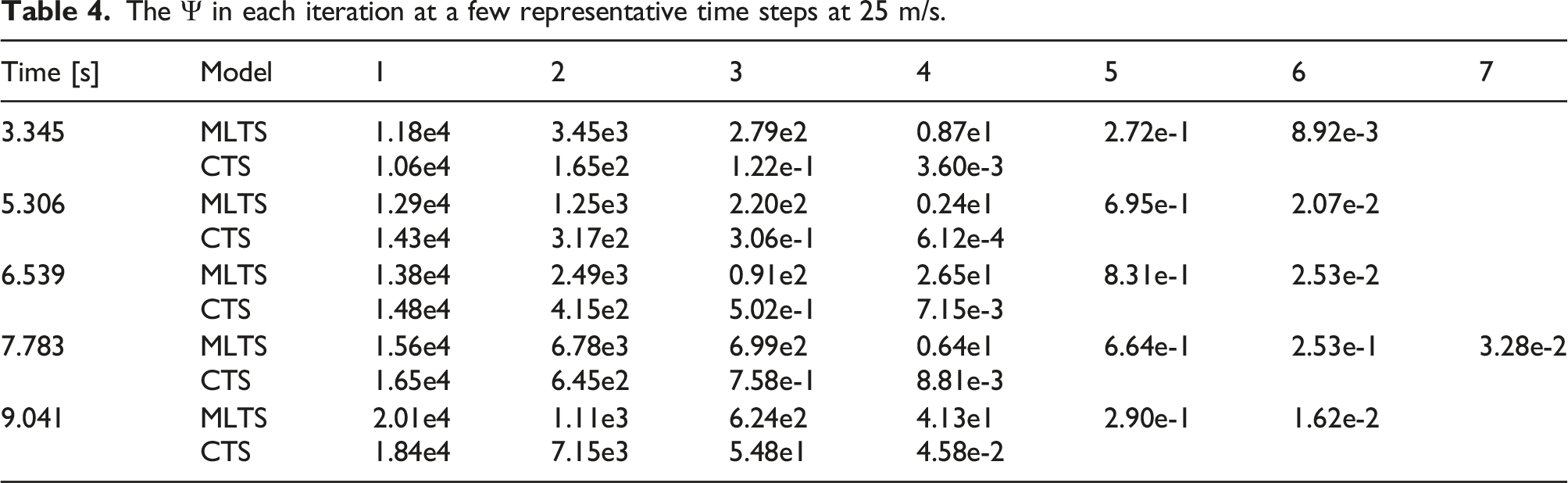
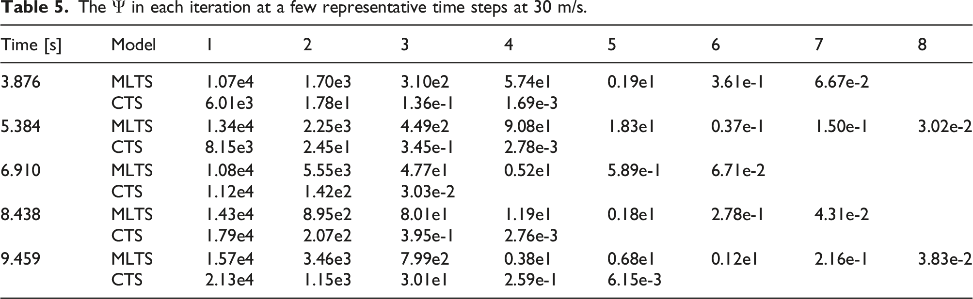
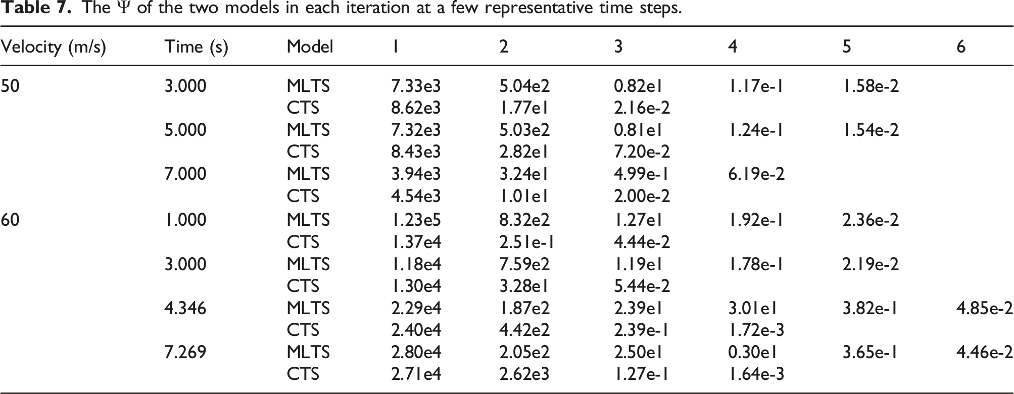
Figure 7 shows the lateral forces of the wheelset. Before the flange hits the rail, the lateral forces calculated by the two models are almost equal, with a difference of less than 0.1%. After about 3.6 s, the lateral forces begin to change abruptly with a period of 0.7 s. The difference of amplitude calculated by two methods is relatively small, for example, 4.3% at 5.1 s (left wheel) and 7.4% at 6.3 s (right wheel). At the moment that the flange has not hit the rail, the response of the lateral forces have high frequency vibration, which can be found in the zoomed view in Figure 7. These results verify the accuracy of the MLTS. Besides, the calculation efficiency of the MLTS method is also verified. The $Ψ$ (see equation (3)) of two methods at special moments are shown in Table 3, where the first three lines represent the moment when the flange does not hit the rail, while the last three lines represent the moment of collision. It shows MLTS requires more iteration numbers than CTS. However, MLTS is still efficient due to the calculation of it is more simplified than that of CTS. The method’s computation time is 306 s, 76.5% less than the 1304 s of the CTS method. It should be noted that those are clock times rather than CPU times, which depend on the hardware and configuration of the computer, such as CPU speed, memory capacity, and background processing. The two models herein run sequentially on a same computer in these tests, so the computation times are comparable.

Figure 7.

Lateral forces $F_{y}$ at the wheel nodes.

Table 3.

Residual of the unbalance force in each iteration at a few representative time steps by using MLTS and CTS.

Time [s]	Model	1	2	3	4	5	6
1.000	MLTS	8.7e3	4.52e2	9.52e1	4.50e-3
1.000	CTS	5.6e3	1.52e2	1.76e-1	2.24e-4
2.000	MLTS	5.56e5	4.86e3	4.57e2	1.59e-2
2.000	CTS	3.58e5	6.89e4	2.14e2	8.47e-2
3.000	MLTS	7.14e5	6.41e4	6.80e2	3.22e-1	2.07e-2
3.000	CTS	6.92e5	5.46e4	3.47e3	3.10e-1	1.01e-3
5.125	MLTS	9.20e3	5.54e2	18.90e1	7.45e-1	3.30e-3
5.125	CTS	6.94e3	1.03e2	1.66e-1	5.29e-4
7.46	MLTS	1.26e5	7.95e3	4.70e2	4.14e1	3.53e-1	3.25e-2
7.46	CTS	1.26e5	2.09e4	9.58e2	2.94e1	9.13e-2
9.598	MLTS	5.48e5	4.25e4	7.80e2	3.15e1	5.42e-1	4.07e-2
9.598	CTS	2.99e5	6.56e4	4.48e3	4.10e-1	2.01e-3

The validated MLTS method is used to predict the response of the model at different velocities, and the results are compared with those of the CTS method. Only the results of the left wheel are listed here for simplicity. Figure 8(a) and (b)) compare the lateral displacements predicted by MLTS with those calculated by the CTS method at 25 m/s and 30 m/s. The results remain very close, though as the velocity increases, the difference slightly increase, especially at the peak where the flange hits the rail. The RMSE of the two models is 0.29 mm at 25 m/s and 0.74 mm at 30 m/s. Figure 8(c) and (d) show the lateral forces predicted by MLTS compared with those calculated by CTS. When the velocity is 25 m/s, the lateral forces of the two models are in good agreement except for a few time steps (i.e., 6.539 s). When the velocity is 30 m/s, the lateral forces of the two are in good agreement in general but not as good as the result of 25 m/s, and the difference becomes more obvious especially after 7s. In a word, the results of the two models are generally close, but become slightly different when the velocity increases. The residual of unbalanced force $Ψ$ in each iteration at a few representative time steps by using MLTS and CTS at 25 m/s (30 m/s) are shown in Table 4 (Table 5). The results show that MTLS requires more iteration steps than CTS. However, MTLS is far less than CTS in terms of total time. When the speed is 25 m/s, the computation time of MTLS is 348 s, which is 69.63% less than 1146 s of CTS. When the speed is 30 m/s, the computation time of MTLS is 346 s, which is 65.60% less than 1006 s of CTS.

Figure 8.

(a) Lateral displacement at 25 m/s; (b) lateral displacement at 30 m/s; (c) lateral forces at 25 m/s; (d) lateral forces at 30 m/s.

Table 4.

The $Ψ$ in each iteration at a few representative time steps at 25 m/s.

Time [s]	Model	1	2	3	4	5	6	7
3.345	MLTS	1.18e4	3.45e3	2.79e2	0.87e1	2.72e-1	8.92e-3
3.345	CTS	1.06e4	1.65e2	1.22e-1	3.60e-3
5.306	MLTS	1.29e4	1.25e3	2.20e2	0.24e1	6.95e-1	2.07e-2
5.306	CTS	1.43e4	3.17e2	3.06e-1	6.12e-4
6.539	MLTS	1.38e4	2.49e3	0.91e2	2.65e1	8.31e-1	2.53e-2
6.539	CTS	1.48e4	4.15e2	5.02e-1	7.15e-3
7.783	MLTS	1.56e4	6.78e3	6.99e2	0.64e1	6.64e-1	2.53e-1	3.28e-2
7.783	CTS	1.65e4	6.45e2	7.58e-1	8.81e-3
9.041	MLTS	2.01e4	1.11e3	6.24e2	4.13e1	2.90e-1	1.62e-2
9.041	CTS	1.84e4	7.15e3	5.48e1	4.58e-2

Table 5.

The $Ψ$ in each iteration at a few representative time steps at 30 m/s.

Time [s]	Model	1	2	3	4	5	6	7	8
3.876	MLTS	1.07e4	1.70e3	3.10e2	5.74e1	0.19e1	3.61e-1	6.67e-2
3.876	CTS	6.01e3	1.78e1	1.36e-1	1.69e-3
5.384	MLTS	1.34e4	2.25e3	4.49e2	9.08e1	1.83e1	0.37e-1	1.50e-1	3.02e-2
5.384	CTS	8.15e3	2.45e1	3.45e-1	2.78e-3
6.910	MLTS	1.08e4	5.55e3	4.77e1	0.52e1	5.89e-1	6.71e-2
6.910	CTS	1.12e4	1.42e2	3.03e-2
8.438	MLTS	1.43e4	8.95e2	8.01e1	1.19e1	0.18e1	2.78e-1	4.31e-2
8.438	CTS	1.79e4	2.07e2	3.95e-1	2.76e-3
9.459	MLTS	1.57e4	3.46e3	7.99e2	0.38e1	0.68e1	0.12e1	2.16e-1	3.83e-2
9.459	CTS	2.13e4	1.15e3	3.01e1	2.59e-1	6.15e-3

A light rail vehicle running over a straight rigid track

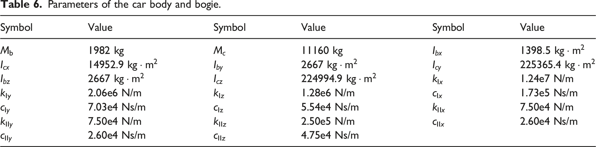
A light rail vehicle (Chopra AK, 1995; Pombo J and Ambrósio J, 2007) running over a straight rigid track (Figure 9) will serve as a more complex example. The model consists of four wheelsets (eight WRI elements), which is the same as that in the Verify the MLTS at various velocities. The primary suspension of the vehicle is simulated by spring-dampers I between the WRI element and the bogie, which appears black in Figure 9. And the secondary suspension is simulated by spring-dampers II between the WRI element and the car body, which appears pink in Figure 9. The bogies and the car body are simulated using elastic beam column elements in OpenSees. The material parameters of the bogie, car body, and suspension are in Table 6, where the subscripts band c denote “bogie” and “car body,” respectively. M denotes the mass and I denotes the area moment of inertia. All of the spring dampers are simulated by two-node link elements in OpenSees, k_I and k_II represent the stiffness of primary and secondary suspensions, and c_I and c_II represent the damping of primary and secondary suspensions. k_I, k_II, c_I, and c_II are all three-dimensional, and the x, y, and z direction in the table is consistent with the GCS. Similar to the previous example, a lateral force is applied to each wheelset in the static analysis so that the lateral displacement of the vehicle is 2 mm. The force is removed at the beginning of the dynamic analysis, and then the hunting motion of the vehicle at different speeds can be studied. Figure 10 shows the lateral displacement of the center of wheelset 1 calculated by the MLTS and CTS methods at 50 m/s and 60 m/s. In order to make the results clear, the data of the CTS method are plotted at regular intervals. The results of the two models agree well at both speeds. At 50 m/s the lateral displacement predictions of the two methods are periodic and the amplitude gradually decreases from 2 mm to 1.36 mm. When the speed is 60 m/s the amplitudes of both methods increase gradually from 2 mm to about 6.97 mm and then remain stable. Figure 11 shows the lateral force on the left wheels of wheelset 1 at 50 m/s and 60 m/s with the CTS predictions plotted at regular intervals. At 50 m/s the lateral force from both methods is periodic with its amplitude gradually decreasing from 1.22 kN to 0.98 kN. At 60 m/s, Figure 11 shows that the two curves almost coincide including at the peak values. Each positive amplitude in Figure 10 corresponds to a peak value in Figure 11, that is, the flange of the left wheel hits the rail at that time.

Figure 9.

Model of a light rail vehicle and a straight rigid track.

Table 6.

Parameters of the car body and bogie.

Symbol	Value	Symbol	Value	Symbol	Value
$M_{b}$	1982 kg	$M_{c}$	11160 kg	$I_{b x}$	$1398.5 kg \cdot m^{2}$
$I_{c x}$	14952.9 $kg \cdot m^{2}$	$I_{b y}$	$2667 kg \cdot m^{2}$	$I_{c y}$	225365.4 $kg \cdot m^{2}$
$I_{b z}$	$2667 kg \cdot m^{2}$	$I_{c z}$	224994.9 $kg \cdot m^{2}$	k _Ix	1.24e7 N/m
k _Iy	2.06e6 N/m	k _Iz	1.28e6 N/m	c _Ix	1.73e5 Ns/m
c _Iy	7.03e4 Ns/m	c _Iz	5.54e4 Ns/m	k _IIx	7.50e4 N/m
k _IIy	7.50e4 N/m	k _IIz	2.50e5 N/m	c _IIx	2.60e4 Ns/m
c _IIy	2.60e4 Ns/m	c _IIz	4.75e4 Ns/m

Figure 10.

Lateral displacement of wheel center at 50 m/s and 60 m/s.

Figure 11.

Lateral force on the left wheels at 50 m/s and 60 m/s.

The computation efficiency of the MLTS method in this case is also verified. Besides, the residual of the unbalanced force

Ψ

of two methods at different velocities are shown in Table 7. The results show MLTS method requires more iteration steps. However, when the velocity of the vehicle is 50 m/s, the total calculation time of the MLTS method is 994 s, 67.7% less than the 3076 s of the CTS method. when the velocity of the vehicle is 60 m/s, the total calculation time of the MLTS method is 1052 s, 69.9% less than the 3498 s of the CTS method. These results demonstrate the efficiency and utility of the MLTS technique in this more complex situation.

Table 7.

The $Ψ$ of the two models in each iteration at a few representative time steps.

Velocity (m/s)	Time (s)	Model	1	2	3	4	5	6
50	3.000	MLTS	7.33e3	5.04e2	0.82e1	1.17e-1	1.58e-2
	3.000	CTS	8.62e3	1.77e1	2.16e-2
	5.000	MLTS	7.32e3	5.03e2	0.81e1	1.24e-1	1.54e-2
	5.000	CTS	8.43e3	2.82e1	7.20e-2
	7.000	MLTS	3.94e3	3.24e1	4.99e-1	6.19e-2
	7.000	CTS	4.54e3	1.01e1	2.00e-2
60	1.000	MLTS	1.23e5	8.32e2	1.27e1	1.92e-1	2.36e-2
	1.000	CTS	1.37e4	2.51e-1	4.44e-2
	3.000	MLTS	1.18e4	7.59e2	1.19e1	1.78e-1	2.19e-2
	3.000	CTS	1.30e4	3.28e1	5.44e-2
	4.346	MLTS	2.29e4	1.87e2	2.39e1	3.01e1	3.82e-1	4.85e-2
	4.346	CTS	2.40e4	4.42e2	2.39e-1	1.72e-3
	7.269	MLTS	2.80e4	2.05e2	2.50e1	0.30e1	3.65e-1	4.46e-2
	7.269	CTS	2.71e4	2.62e3	1.27e-1	1.64e-3

Conclusions

The element tangent stiffness, defined as the differentiation of element insisting force to nodal displacement, is important to in calculation efficiency when Newton’s method is used to solve implicit nonlinear finite element equations. This paper represents a machine learning based tangent stiffness (MLTS) calculation method, and applies it to a complicated three-dimensional wheel-rail interaction (WRI) element. The displacement and the velocity of the wheel node are the input and the entries of the tangent stiffness are the output. The MLTS are obtained by an artificial neural network (ANN) using error back-propagation (BP) algorithm and the trained model is implemented in an open source finite element (FE) software framework that is widely used in civil engineering, OpenSees. A wheelset example running on the rigid rail is used to verify the accuracy and efficiency of the MLTS. The displacement, velocity and acceleration responses of wheelset are compared with those calculated by consistent tangent stiffness (CTS) and the accuracy of the WRI element using MLTS is verified. Besides, the iterative steps required to achieve convergence and the total calculation time required for the two methods are compared. Although MLTS needs slightly more convergence iterations, it still has a huge efficiency advantage, and the total computing time is reduced by 76.5%. The same wheelset example with different velocities are also considered in this paper, the accuracy of WRI element using MLTS decreases with the increase of speed, but it is still reliable. The calculation efficiency is 69.63% (25 m/s) and 65.60% (30 m/s) higher than that of CTS. In addition, a light rail vehicle running over a straight rigid track is considered to verify the applicability of the MLTS derived in this paper. The response calculated by MLTS is almost consistent with that calculated by CTS. Similar to the wheelset example, the WRI element using MLTS needs more iterative steps but greatly improves the calculation efficiency, increasing 67.7% (50 m/s) and 69.9% (60 m/s) than that of CTS, respectively. The results demonstrate that machine learning based element tangent stiffness method presented herein are efficient, reliable, and acceptably accurate and can be used in complicated vehicle-track systems.

Footnotes

Acknowledgments

The funding support by National Natural Science Foundation of China (51978591) is gratefully acknowledged.

Declaration of conflicting interests

The author(s) declared no potential conflicts of interest with respect to the research, authorship, and/or publication of this article.

Funding

The author(s) disclosed receipt of the following financial support for the research, authorship, and/or publication of this article: This article was supported by National Natural Science Foundation of China (grant no: 51978591).

ORCID iD

Surong Huang

References

Acikbas

Soylemez

(2008) Coasting point optimisation for mass rail transit lines using artificial neural networks and genetic algorithms. IET Electric Power Applications 2(3):172–182.

Chen

Zhai

(2004) A new wheel/rail spatially dynamic coupling model and its verification. Vehicle System Dynamics 41(4): 301–322.

Chopra

(1995) Dynamics of Structures: Theory and Applications to Earthquake Engineering. USA: Prentice-Hall.

Dietterich

(1998) Approximate statistical tests for comparing supervised classification learning algorithms. Neural Computation 10(7): 1895–1923.

Dinh

Kim

Warnitchai

(2009) Dynamic analysis of three-dimensional bridge-high-speed train interactions using a wheel-rail contact model. Engineering Structures 31(12): 3090–3106.

Doghri

(1993) Fully implicit integration and consistent tangent modulus in elastoplasticity. International Journal for Numerical Methods in Engineering 36(22): 3915–3932.

Conte

Yang

(2011) Consistent tangent moduli for multi-yield-surface J(2) plasticity model. Computational Mechanics 48(1): 97–120.

Liu

Guo

, et al. (2019) A practical wheel-rail interaction element for modeling vehicle-track-bridge systems. International Journal of Structural Stability and Dynamics 19(2): 1950011.

Pan

Liu

(2021) Consistent tangent stiffness of a three-dimensional wheel-rail interaction element. International Journal of Structural Stability and Dynamics 21(14): 2140010.

10.

Hertz

(1882) On contact between elastic bodies. Journal Fur Die Reine Und Angewandte Mathematik 92: 156–171.

11.

Huang

Loh

(2001) Nonlinear identification of dynamic systems using neural networks. Computer-aided Civil and Infrastructure Engineering 16(1): 28–41.

12.

Jirasek

Patzak

(2002) Consistent tangent stiffness for nonlocal damage models. Computers & Structures 80(14–15): 1279–1293.

13.

Jung

Ghaboussi

(2006) Neural network constitutive model for rate-dependent materials. Computers & Structures 84(15): 955–963.

14.

Kang

Liu

(1997) Concrete dam deformation prediction model for health monitoring based on extreme learning machine. Structural Control & Health Monitoring 24(10): e1997.

15.

(2015) Prediction of railcar remaining useful life by multiple data source fusion. IEEE Transactions On Intelligent Transportation Systems 16(4): 2226–2235.

16.

Liu

Montenegro

, et al. (2021) A practical three-dimensional wheel-rail interaction element for dynamic response analysis of vehicle-track systems. Computers & Structures 254: 106581.

17.

Luo

Paal

(2018). Machine learning-based backbone curve model of reinforced concrete columns subjected to cyclic loading reversals. Journal of Computing in Civil Engineering 32(5): 04018042.

18.

Magalhaes

Marques

Liu

, et al. (2020). Implementation of a non-Hertzian contact model for railway dynamic application. Multibody System Dynamics 48(1): 41–78.

19.

Marques

Magalhaes

Pombo

, et al. (2020). A three-dimensional approach for contact detection between realistic wheel and rail surfaces for improved railway dynamic analysis. Mechanism and Machine Theory 149: 103825.

20.

Marques

Magalhaes

Liu

, et al. (2019) On the generation of enhanced lookup tables for wheel-rail contact models. Wear 434: 202993.

21.

Miehe

(1996) Numerical computation of algorithmic (consistent) tangent moduli in large-strain computational inelasticity. Computer Methods in Applied Mechanics and Engineering 134(3–4): 223–240.

22.

Mohammadi

Ghofrani

, et al. (2019) Exploring the impact of foot-by-foot track geometry on the occurrence of rail defects. Transportation Research Part C-Emerging Technologies 102: 153–172.

23.

Mordecai

(2003) Nonlinear Programming: Analysis and Methods. NY, USA: Dover Publishing.

24.

Planinc

Saje

(1999) A quadratically convergent algorithm for the computation of stability points: the application of the determinant of the tangent stiffness matrix. Computer Methods in Applied Mechanics and Engineering 169(1–2): 89–105.

25.

Polach

(1999) A fast wheel-rail forces calculation computer code. Vehicle System Dynamics 33: 728–739.

26.

Pombo

(2004) A Multibody Methodology for Railway Dynamics Applications. Ph.D Thesis, Lisbon University of Technology, Portugal.

27.

Pombo

Ambrosio

(2005) Dynamic analysis of a railway vehicle in real operation conditions using a new wheel-rail contact detection model. International Journal of Vehicle Systems Modelling and Testing 1(1/2/3): 79–105.

28.

Pombo

Ambrósio

(2007) Modelling tracks for roller coaster dynamics. International Journal of Vehicle Design 45(4): 470–500.

29.

Pombo

Ambrósio

Silva

(2007) A new wheel–rail contact model for railway dynamics. Vehicle System Dynamics 45(2): 165–189.

30.

Shabana

Zaazaa

Sugiyama

(2008) Railroad Vehicle Dynamics: A Computational Approach. Boca Raton, USA: CRC Press.

31.

Simo

Taylor

(1985) Consistent tangent operators for rate-independent elastoplasticity. Computer Methods in Applied Mechanics and Engineering 48(1): 101–118.

32.

Wang

Zhuang

Zhang

(2019) Automatic detection of rail surface cracks with a superpixel-based data-driven framework. Journal of Computing in Civil Engineering 33(1): 04018053.

33.

Zhai

(2004) Two simple fast integration methods for large-scale dynamic problems in engineering. International Journal for Numerical Methods in Engineering 39(24): 4199–4214.

34.

Zhai

Cai

Guo

(1996) Coupling model of vertical and lateral vehicle/track interactions. Vehicle System Dynamics 26(1): 61–79.

35.

Zhai

Wang

Cai

(2009) Fundamentals of vehicle-track coupled dynamics. Vehicle System Dynamics 47(11): 1349–1376.