
Abstract
Multitudes of algorithms have been proposed to evaluate the failure probability of components and systems. Among all these algorithms, direction sampling is a promising one. However, a major computational effort involved in direction sampling is that for each direction sample a root-searching process needs to be conducted to obtain the distance between the origin and the failure surface, which can be computationally expensive. In addition, the failure probability along a direction is hard to obtain when the direction vector intersects the failure surface multiple times. This paper proposes a novel approach to obtain densely populated points locating on the failure surface and utilizing these points to conduct reliability analysis with direction sampling. The process of obtaining the population consists in dividing the initial hypercube space into multiple lattice grids, identifying the grids crossing the failure surface, and dividing these grids into smaller ones. The iterative division process stops when the grids cut across by the failure surface are small enough so that the centers of these grids can be considered located on the failure surface. Several numerical tests are performed to validate the applicability of the proposed approach. Through these tests, it can be concluded that for the situation where the intersection between the direction vector and the failure surface is unique, the proposed approach will lead, with high accuracy, to a failure probability. For the situation where the intersection is not unique, satisfactory estimation of failure probabilities can also be achieved using approximation methods. For high-dimensional reliability problems, clustering techniques can be utilized to reduce the computational cost.
Introduction
Structural reliability analysis is a classic research problem with a long history. The analysis result provides a sound estimation of the structural performance under load effects and possibly multiple deterioration mechanisms, which serves as the basis to lay out intervention strategies during the life-cycle of structures. By definition, the failure probability of a structure is
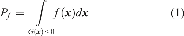
Different methodologies have been proposed to circumvent the integration in equation (1). Among these methodologies, approximation approach such as the First Order Reliability Method (FORM) and Second Order Reliability Method (SORM) are widely adopted, especially FORM. In FORM, the performance function is approximated at the most probable point (MPP) with first order Taylor series (i.e., linear function). MPP is a point located on the failure surface (i.e., G(
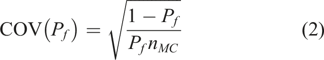
Sampling methods are another school-of-thought to tackle the reliability problem. The most basic sampling method is crude Monte Carlo (MC) simulation. Large numbers of samples of random variables are generated to evaluate the associated values of performance functions. The failure probability is determined as the ratio of the number of samples resulting in negative values of performance function (indicating the failure of the structure) over the total number of generated samples. For sampling methods, different trials using the same number of samples can result in different probabilities of failure. The coefficient of variation of the failure probability obtained using crude MC simulation, COV(P
f
), is expressed as (Melchers, 1987)
Quantities of smart sampling techniques have been proposed to reduce the number of samples needed to achieve a satisfactory level of accuracy, such as stratified sampling (a well-known type of stratified sampling is Latin hypercube sampling (McKay et al., 1979)), importance sampling (Tokdar and Kass, 2010), and subset simulation (Au and Beck, 2001). Song and Kawai (2023) proposed an adaptive stratified sampling method to conduct structural reliability analysis. Zuniga et al., (2021) integrated dimension reduction techniques into importance sampling approach to conduct structural reliability assessment. Although Latin hypercube sampling can reduce the number of samples, the number of samples needed are still large. For importance sampling, the region of importance needs to be identified which may be a tricky issue in itself. Subset sampling involves an iterative process which can be time-consuming although the number of samples needed is reduced. In addition, subset sampling has some limitations in terms of applicability (Breitung, 2017).
Direction sampling (Ditlevsen and Bjerager, 1986) and line sampling (Koutsourelakis et al., 2004; Schuëller et al., 2004) are two sampling methods taking the geometry of the failure surface into consideration. These two methods are also conducted in the U-space. Direction sampling approach involves uniformly generating direction samples on the unit hypersphere. The one-dimensional reliability index along each direction is associated with the distance from the origin to the intersection point between the direction vector and the failure surface. The distance can be determined by searching the root of a unit-variate equation. Line sampling, on the other hand, identifies an important direction and generates samples on the hyperplane perpendicular to the important direction. An issue with using line sampling is how to identify this importance direction. Given this issue, more robust line sampling techniques have been proposed, such as the adaptive line sampling (Pradlwarter et al., 2007) and combined line sampling (Papaioannou and Straub, 2021), among others. Recent studies have proposed new algorithms based on the direction sampling method and line sampling method, such as Cheng et al., (2023) and Jafari-Asl et al. (2021), among others. Overall, the direction sampling approach is preferred over the line sampling approach as the former skips the direction determination process which can be complicated. However, a weakness shared by both direction sampling and line sampling lies in the root-searching process. The associated one-variate equation can be highly nonlinear, and the roots can be multiple. Due to this weakness, direction sampling is widely applied only for reliability problems associated with simple-connected failure regions.
It is worth noting that using surrogate models to conduct reliability analysis is another type of approach. Surrogate models are used to represent the original performance functions that is very complex or implicit. Sampling methods are then utilized to obtain the failure probability associated with the surrogate model. Two major research aspects on the surrogate model approach are the metamodels used to fit the data and the learning function. Metamodels considered in the surrogate models includes polynomial response surface (Bucher and Bourgund, 1990; Faravelli, 1989), polynomial chaos expansions (Ghanem and Spanos, 1991), and Kriging (Vahedi et al., 2018; Wang et al., 2022), among others. Learning functions to obtain the design of experiment (the point on the exact failure surface, abbreviated as DoE) include expected feasibility function (EFF) (Bichon et al., 2008), U-function (Echard et al., 2011), and least improvement function (LIF) (Sun et al., 2017), among others. It is worth mentioning that several studies have integrated surrogate models with smart sampling approach, such as Zhang et al., (2020) and Nguyen et al., (2022), among others. The philosophy of surrogate models is to obtain an accurate reliability analysis result while minimizing the number of DoEs used to conduct the parameter fitting. As the number of DoEs is limited, there is some discrepancy between the function used in the surrogate model and the original performance function, which is the source of error associated with this type of approach. In addition, an iterative method is also needed in the process of fitting the surrogate model, which may be time-consuming.
Vast amounts of research effort have been devoted to the calculation of failure probability of structures. It should be noted that information on the configuration of failure surface is also beneficial. A primary benefit of knowing the configuration of the failure surface is that when the values of some random variables are identified through structural health monitoring (SHM) techniques, the failure probability can be updated with ease without carrying out new reliability analyses. For instance, for a bridge structure subjected to dead and live loads, the uncertainties associated with the dead loads, live loads, and resistances are involved in the reliability analysis processes. If the failure surface is identified, the time-variant failure probability is known instantly if live load effects are measured using weigh-in-motion (WIM) systems. For a steel structure subjected to corrosion-enhanced fatigue, the fatigue reliability involves the uncertainties associated with both corrosion modelling and fatigue modelling. The fatigue reliability can be updated with ease when the stress histogram is obtained using SHM if the failure surface of the structure subjected to corrosion-enhanced fatigue is known. In addition, failure surface can help pinpointing the critical regions of values of random variables that lead to the failure of the structure, such as the region around the most probable point (MPP) which is sought in FORM.
This paper proposes a novel approach to tackle the reliability problem, which is to obtain densely populated points on the failure surface and use them to conduct reliability analysis with the direction sampling technique. For each generated direction sample, the point to which the direction from the origin in the U-space is closest to the direction sample is selected. The distance from the point to the origin in the U-space is considered as the reliability index along the direction of the sample if the intersection point is unique. For the case where a direction vector has multiple intersection points with the failure surface, an approximation method is proposed to obtain all the intersection points. In addition, clustering techniques can be utilized to reduce the computational expense when the dimensionality of the reliability problem is high. The novelty of this approach lies in using the densely populated points to infer the intersections between direction vectors and failure surfaces. Using this approach to solve the reliability problem associated with multiple intersections between the direction vectors and the failure surface as well as integrating clustering techniques into this approach further enhances the novelty of this study. Several examples are investigated to verify the validity of this approach. The flowchart of the proposed approach is shown in Figure 1. Flowchart of the proposed reliability approach.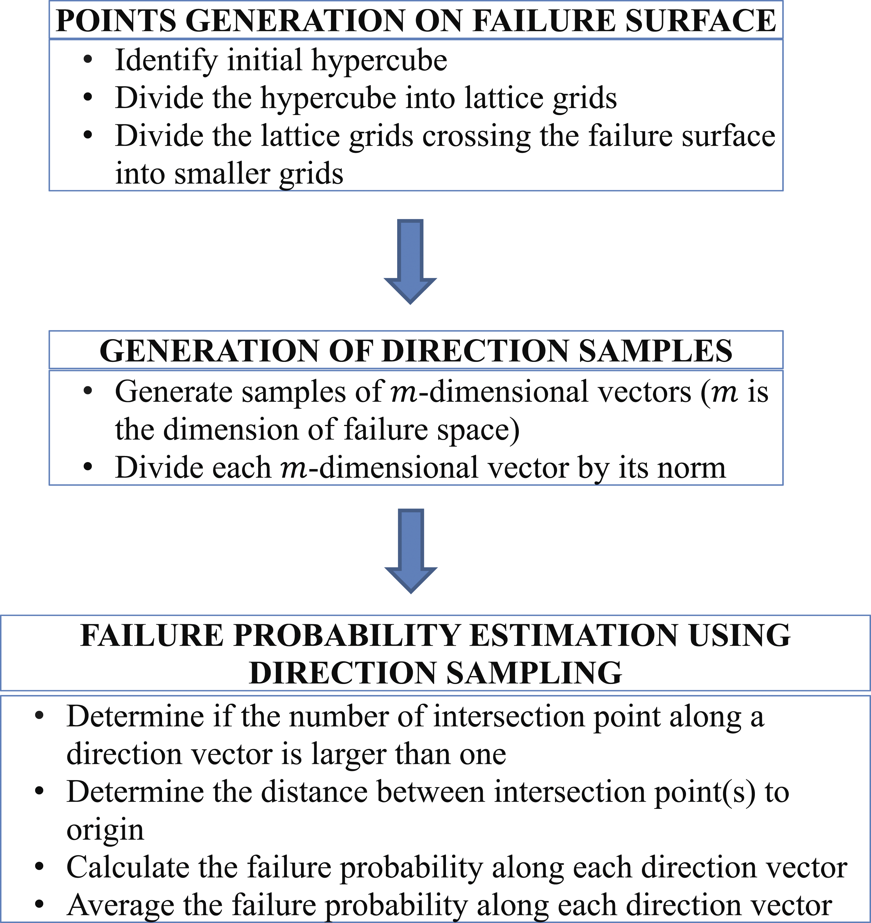
Theoretical background of direction sampling
In the space of the independent standard normal random variables (i.e., the U-space), the shape of the joint PDF ϕ
u
(
An m -dimensional independent standard normal vector
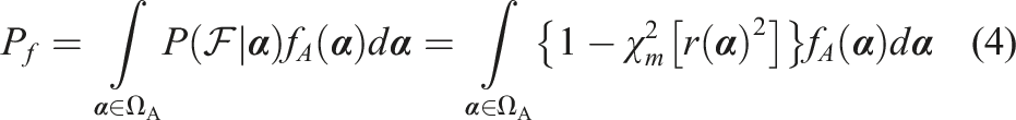
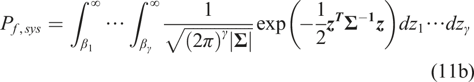
The failure probability in equation (1) can be rewritten as
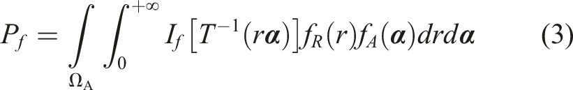
If Monte Carlo simulation is conducted using equation (3), the computation effort will be similar to that using samples generated based on Cartesian coordinates. An alternative methodology based on the concept of conditional probability was proposed in Ditlevsen and Bjerager (1989), which is expressed as
Novel approach to conduct reliability analysis
The key concept of the novel approach to conduct reliability analysis is to obtain densely populated points on the failure surface in the U -space. When the points are obtained, for each direction vector pointing from the origin, it is possible to find the point very close to vector and consider this point as the intersection between the direction vector and the failure surface, thereby eliminating the root-searching process. The random variables that are not standard normal can be converted into standard normal random variables using Rosenblatt or Nataf transformation (Melchers, 1987). The approach is divided into two parts: (i) obtaining the lattice grids crossing the failure surface that are small enough so that the center of gravity of these grids can be considered as locating on the failure surfaces, and (ii) utilizing direction sampling to obtain the failure probability.
Division of lattice grids
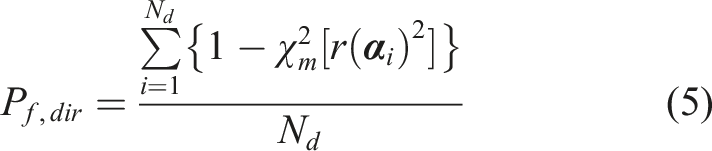
The procedure of obtaining the small lattice grids crossing the failure space is as follows: • Step 1: Identify a hypercube space in the m -dimension U -space. The hypercube space is defined as • Step 2: Determine if a grid crosses the failure surface. This process is conducted by using the values of the performance function at the vertices of the grid and randomly generated points within the grid. • Step 3: Ignore the grids that do not cross the failure surface. Divide all the grids crossing the failure surface into smaller grids. The division is performed by dividing the segment of a grid into two parts in each dimension. After the division, each new grid is associated with one-half of the length of the divided grid in each dimension (i.e., Uint,in = Uint,i/2, where Uint,in is the new grid interval in the i th dimension). • Step 4: Return to step 2 unless all the grids crossing the failure surface are small enough. Illustration of a three-dimension cube divided using lattice points.
The lower and upper bounds of the hypercube in each dimension (U li and U bi , i = 1,…,m) and the length of lattice grid in each dimension (Uint,i; i = 1,…,m) are user-specified. Theoretically, a larger initial hypercube can help capture the failure surface more thoroughly, especially the regions in the failure surface that are distant from the origin. However, as the contribution of the far-away regions in the failure surface to the failure probability is small, capturing these regions may not improve the accuracy of the calculated failure probability significantly. In addition, a large initial space may incur a heavy burden of computational cost. Therefore, a balance between the accuracy and the computational cost should be made by the users regarding the initial hypercube space. The initial Uint,i needs not to be small, although a smaller Uint,i can also help characterizing the failure surface more accurately.
It is self-evident that a grid crossing the failure surface is split into two parts by this surface. Therefore, points inside the grid crossing the failure surface can render the value of the performance function both positive and negative. On the other hand, for a grid not crossing the failure surface, the points inside it can only make the value of the performance function positive or negative. A grid can be considered as crossing the failure surface when the points within it are associated with both positive and negative values of the performance function. A simple approach to determine if a grid crosses the failure surface is to evaluate the performance function at the vertices of the performance functions. If both positive and negative values are obtained, then it can be determined that the grid crosses the failure surface. However, it should be noted that if all the values of the performance function at vertices are positive/negative, it is still possible that the failure surface crosses the grid. Therefore, sample points inside the grid need to be generated to determine if a grid crosses the failure surface. It is acknowledged that adding points inside the grid may still fail to determine if a grid crosses the failure surface correctly, although this possibility decreases with the increase of number of sample points. The number of samples should be related to the size of the grid. The larger the size of a grid is, the larger the number of samples should be adopted. For the value of the number of samples generated within a grid N s , a balance should be achieved between the probability of accurate detection and the acceptable computational cost.
Apparently, a specific criterion should be set up to define the smallest grid. For a m-dimension grid, the criteria should be related to the length of the grid in each dimension (i.e., Uint,i;i = 1,…,m). Assuming the lengths of grid in each dimension are equal (Uint,i = Uint,j = U
int
, i≠j), the iterative process stops when U
int
≤ϵ. The smaller ϵ is, the more accurately the failure surface can be represented using the centers of the grids. As a smaller ϵ also implies a larger computational expense, a tradeoff between the accuracy in portraying the failure surface and computational cost should be achieved. In this paper, when the lengths of a grid in each dimension are equal, the number of samples N
s
used to determine if a grid intersects the failure surface is expressed as

It is worth noting that for system reliability analysis involving multiple performance functions, an equivalent performance function can be derived based on the system model. Assuming n
g
performance functions

For a parallel system, the equivalent performance function is

Direction sampling using the center of grids
After the small grids crossing the failure surface are obtained, the centers of these grids are used in the direction sampling process. Depending upon the number of intersections between a direction vector and the failure surface, the following two cases are discussed separately. • Case A: The failure surface and the direction vector only intersect at one point.
In this case, as the centers of grids are densely populated on the failure surface, one of these centers can be considered as the intersection point between the direction vector and the failure surface. For a center of grid, a vector
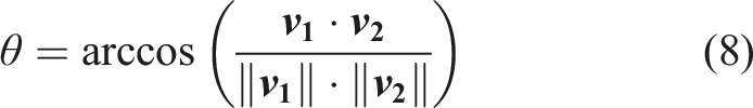
Let the smallest cross angle obtained be θ
s
. If θ
s
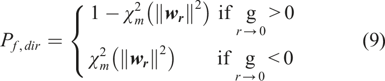
is larger than a specific threshold (referred to as θs,th ), the direction vector can be considered as not crossing the failure surface and the failure probability along this direction is zero. Otherwise, the failure probability along the direction vector is (Melchers, 1987) • Case B: The failure surface and the direction vector intersect at multiple points.
The problem becomes much more complex when multiple intersection points exist between the direction vector and the failure surface. The reason for the existence of multiple intersection points is that either the failure region is enclosed or there are holes in the failure region. An illustration of this scenario is shown in Figure 3(a). Depending upon the sign of (a) Illustration of multiple intersection points between a direction vector and failure surface; (b) illustration of two close intersection points between a direction vector and failure surface.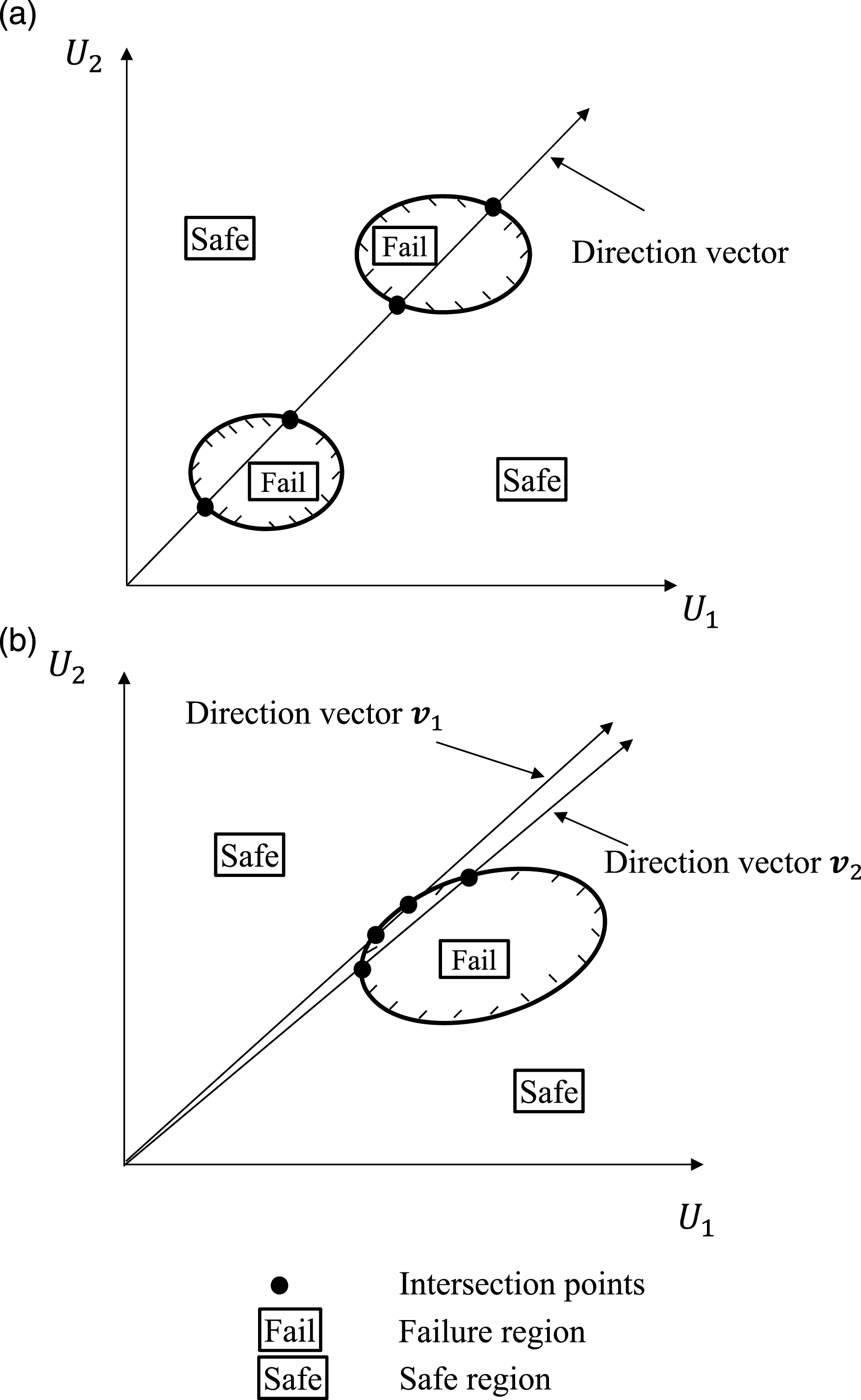
Scenario B1:
In this scenario, the intersection points between a direction vector and the failure surface are odd-numbered. Assuming the distances from the origin to the failure surface along the direction vector are r1,r2,…,r2k+1(k = 1,2,…) in the ascending order, the failure probability along the direction vector is
Scenario B2:
In this scenario, the intersection points between a direction vector and the failure surface are even-numbered. Assuming the distances from the origin to the failure surface along the direction vector are r1,r2,…,r2k(k =1,2,…) in the ascending order, the failure probability along the direction vector is
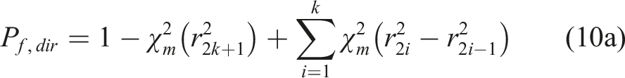
Scenario B3:
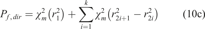
In this scenario, the intersection points between a direction vector and the failure surface are odd-numbered. Assuming the distances from the origin to the failure surface along the direction vector are r1,r2,…,r2k+1(k = 1,2,…) in the ascending order, the failure probability along the direction vector is
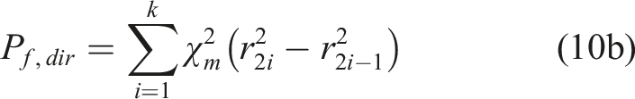
Scenario B4:
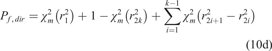
In this scenario, the intersection points between a direction vector and the failure surface are even-numbered. Assuming the distances from the origin to the failure surface along the direction vector are r1,r2,…,r2k(k = 1,2,…) in the ascending order, the failure probability along the direction vector is
The methodology of finding multiple r is detailed as follows: • Step 1: Identify the center of grid associated with the smallest cross angle with the direction vector. This center of grid, • Step 2: For all the vectors • Step 3: Among all the centers of grids in • Step 4: Consider these • Step 5: Repeat step 3 until • Step 6: Sort all the intersection points identified based on their distances from the origin. The reason to conduct the sorting is that the first identified
The value of θ
th
should be small enough so that all the centers of grids that are approximately in the same direction as the direction vector can be identified. The value of θ
th
is also dependent upon the value of ϵ. In fact, θ
th
can be set equal to θs,th. The value of r
th
should be large enough so that centers of gravity that are near the selected intersection point and yet not the real intersection points can be filtered out. Based on numerical experiences, r
th
should be several times larger than θs,th. It should be noted that there are cases where the direction vector is almost tangent to the failure surface (an illustration in this regard is provided in Figure 3(b)). In this case, some intersection points may fail to be detected by the methodology indicated previously. Two different approaches are proposed when this scenario occurs. The first, denoted as approximation approach I, considers the failure probability associated with the direction vector of which the intersection points fail to be detected in full as zero. The other, denoted as approximation approach II, considers the failure probability associated with the original direction vector to be the same as the failure probability associated with a substitute direction vector. The substitute direction vector is selected among all the direction vectors of which the intersection points are successfully identified as the one with the smallest cross angle with the original direction vector. In Figure 3(b), assuming the intersection points between direction vector
Criteria can be proposed regarding if the intersection between a direction vector and the failure surface is unique or not. For a series system reliability problem, it can be asserted that the intersection between a direction vector and the failure surface is unique. For a component reliability problem of which the performance functions involve nonperiodic functions, such as polynomial performance functions, it is likely that intersection between a direction vector and the failure surface is unique. For a component reliability problem associated with performance functions involving periodic functions such as trigonometric functions and parallel system reliability problem, the intersection between a direction vector and the failure surface may not be unique. Monotonicity analysis of the performance functions can be carried out to determine if the intersection point is unique or not.
Using clustering algorithms to reduce the computational cost
It is acknowledged that as the dimension of the performance function increases, the size of the matrix containing the centroids of the grids can increase substantially. Storing such matrices when the grid size is small requires large computer memory and therefore represents a major obstacle for the implementation using the proposed algorithm. For the case where the intersection between a direction vector and the failure surface is unique, clustering techniques can be used to reduce the computational cost and expedite the calculation process. By using clustering techniques, the centroids of grids crossing the failure surface are divided into multiple clusters and only the clusters of grids for which the direction is close to the generated direction samples are selected and continue to be divided.
The procedure of using clustering algorithms to accelerate the calculation process is as follows: • Step 1: Divide the grids crossing the failure surface until the length of the grid U
int
= ϵ1 (assuming the length of the grid in each dimension is identical). • Step 2: Separate the grids into N
k
clusters. For each cluster, calculate the coordinate of each centroid. This coordinate can be considered as a vector, with the origin and the centroid considered as the initial point and terminal point of a vector, respectively. The set of the vectors representing the centroids of all the clusters is denoted as • Step 3: For a specific direction sample, calculate cross angles of this direction sample with each vector in • Step 4: Select N
ks
clusters of grids based on the sorting results, i.e., only the clusters associated the first N
ks
cross angles in the ascending order are selected. • Step 5: Continue dividing the girds in the selected clusters until the final size threshold ϵ is reached. • Step 6: Compute the failure probability along this direction using equations (8) and (9). • Step 7: Repeat Steps 1–6 for all direction samples.
A flowchart of this procedure is shown in Figure 4. Clustering techniques aim to divide a cloud of spatial points into multiple clusters, with the purpose of minimizing the sum of variances of clusters (the variance of a cluster is the sum of square of point-to-cluster-centroid distances) (Du et al., 1999). K-means clustering algorithm (Hartigan and Wong, 1979), a widely used machine learning algorithm, is adopted herein to implement the clustering process. Theoretically, the larger the number of selected clusters N
ks
is, the higher the accuracy of the proposed approach is. However, a larger N
ks
also indicates a larger computational cost. Therefore, the value of N
ks
is user-specified, depending upon the acceptable computational cost as well as the required accuracy of the users. The number of total clusters N
k
is also user-specified. When N
ks
is fixed, a larger N
k
signifies a lower computational cost. However, a larger N
k
corresponds to a longer duration to complete the clustering process. Flowchart of the proposed approach integrating clustering techniques.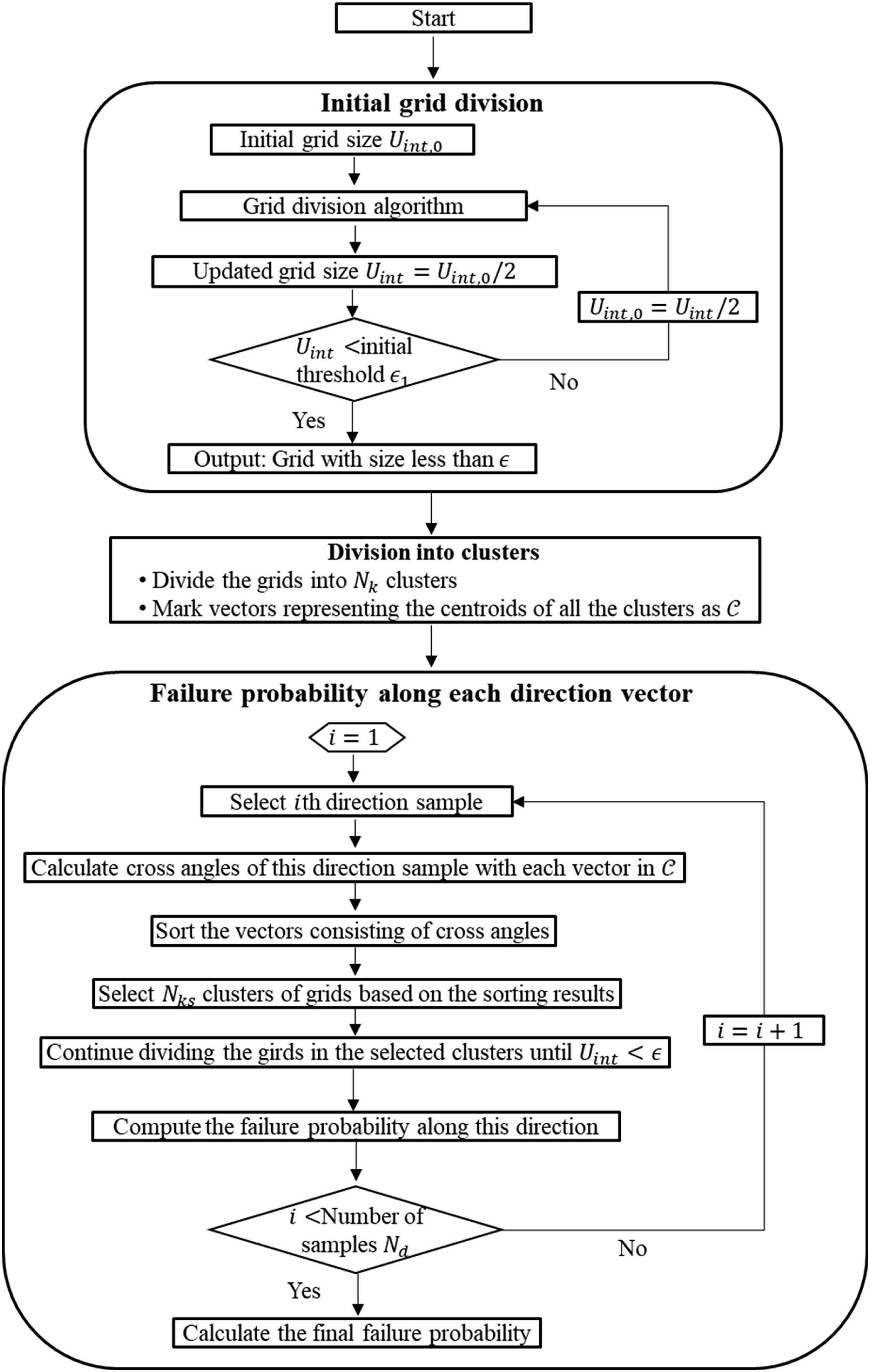
Illustrative examples
To check the applicability of the proposed reliability analysis approach, six example problems are investigated herein. All the example problems investigated herein were considered in previous studies, where reliable results of reliability analysis were provided. To verify the results obtained using this approach, four different methods are considered herein, namely • Method A: The approach proposed herein with 104 direction samples. • Method B: Crude Monte Carlo simulation with 106 samples. • Method C: First Order Reliability Method (FORM) • Method D: Adaptive Kriging Monte Carlo Method (AK-MCS) (Echard et al., 2011)
Both Methods B and C are widely-used approaches to obtain failure probability. Method D is a metamodel-based approach combining Monte Carlo simulation with Kriging metamodels. Comparison between the results of Method A with those associated with Methods B, C, and D can indicate whether the result of the approach proposed herein is reliable.
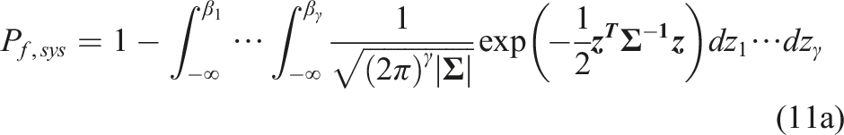
It should be noted that FORM can only obtain the reliability index of individual components. For system reliability, FORM needs to be integrated with the cumulative distribution function (CDF) of multi-variate normal distribution. For a series system of γ failure modes, the failure probability is calculated as (Hohenbichler and Rackwitz, 1982)
For a parallel system of γ failure modes, the failure probability is calculated as (Hohenbichler and Rackwitz, 1982)
For Method D, the learning function and the convergence criteria are based on Echard et al., (2011). The number of samples in the initial DoE and the number of samples added to the experimental design are 10 and 1000, respectively. The number of Monte Carlo samples in Method D is 105. In the last example, reliability analysis integrating clustering techniques is presented.
Example 1: Component reliability problem with linear performance functions
The linear performance functions investigated in Katsuki and Frangopol (1994) are adopted as the first example. These performance functions are:


The three-dimension (3D) case (i.e., g2 ) is used to illustrate the procedures of calculating failure probability in Method A. For each dimension of the hypercube, the lower bound U
l
, upper bound U
b
, and the initial size the of grid U
int
are set as 0, 4, and 2, respectively. N
r
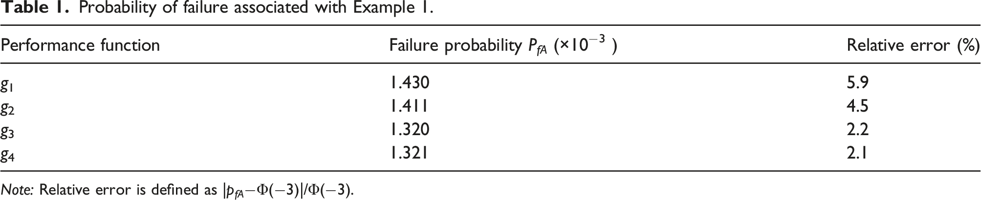
is set as one while ϵ is 0.1. The initial grid plot, the grids crossing the failure surface after the first grid division, and the centers of final grids crossing the failure surface are shown in Figure 5. It can be seen that the linear failure surface can be represented by densely populated centers of grids crossing the failure surface. Apparently, a direction vector can only intersect the failure surface once for this problem. Setting θs,th as 0.1, the failure probabilities using Method A associated with these four performance functions and the relative errors (defined as Illustrations of grid division process for the 3D case in Example 1. (a) Initial grid plot. (b) Grids crossing failure surface after first division. (c) Centers of final grids crossing failure surface. Probability of failure associated with Example 1. Note: Relative error is defined as |p
fA
−Φ(−3)|/Φ(−3).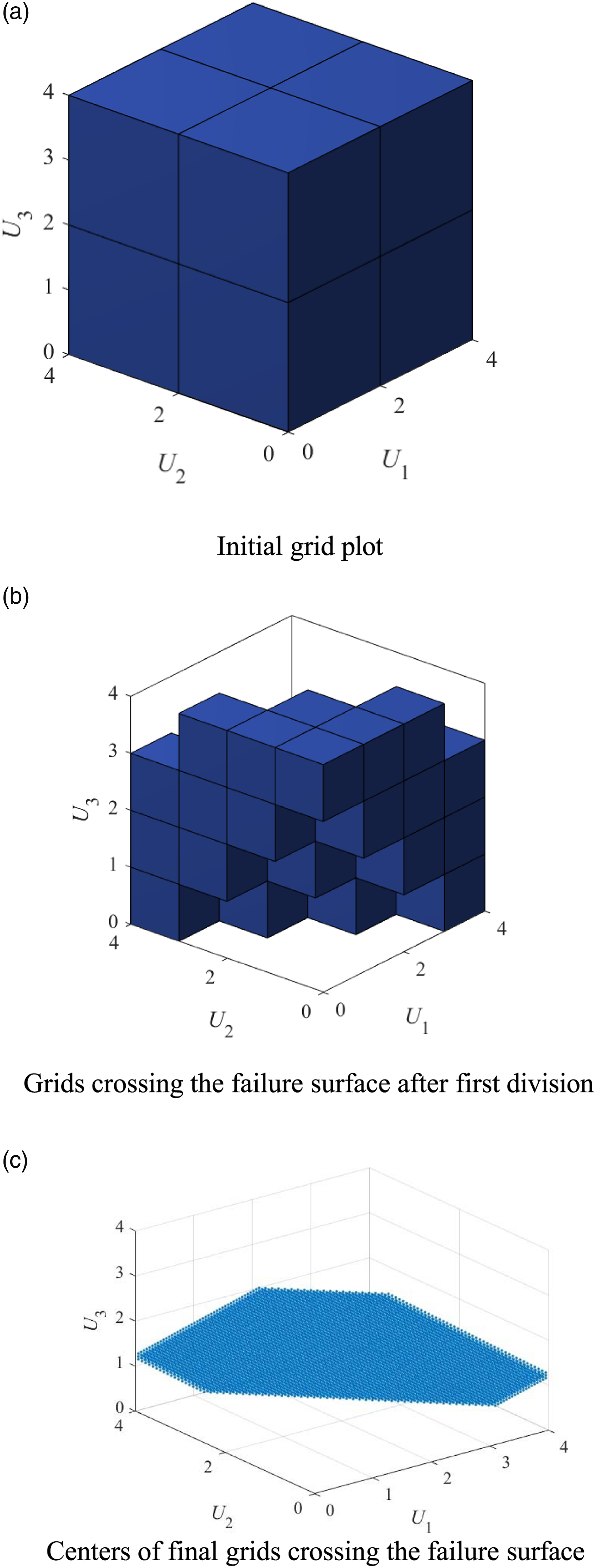
An analysis is carried out using the 2D case to illustrate the effect of number of samples to conduct the simulation associated with Methods A and B on the failure probability results. The relationship between the number of samples used and the obtained failure probability is shown in Figure 6. For this specific case, it can be seen that the dispersion of failure probability is small after the number of samples reaches 104 in Method A, which can prove that the number of samples used herein for Method A (i.e., 104) is sufficient to obtain an accurate failure probability. On the other hand, if Method B is used, the failure probability stabilizes after the number of samples reaches 2 × 10⁵. It can be observed that for the problem associated with a small failure probability, using direction sampling leads to a reduced number of samples compared with using crude MC sampling. Effect of the number of samples used in Methods A and B on the failure probability. (a) Method A, (b) Method B.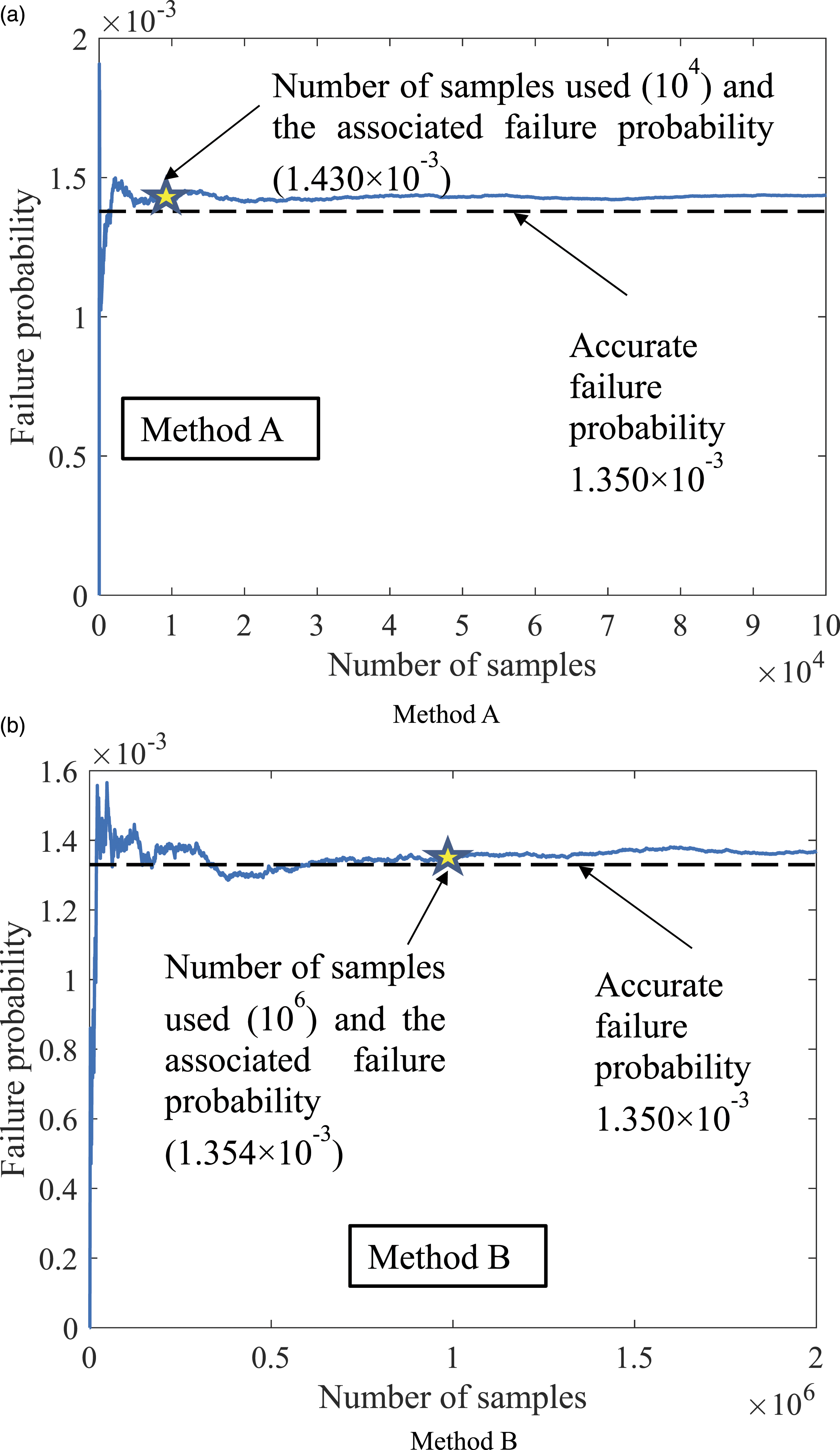
Example 2: Component reliability problem with nonlinear performance function
The second example is associated with a nonlinear performance function, which is expressed as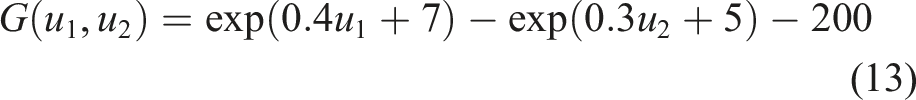
For this problem, the initial space is set as [−4, 4]×[−4, 4]. U
int
and ϵ are set as 2.5 and 0.1, respectively. N
r
and θs,th are set as 1 and 0.1, respectively. The grids crossing the failure surface after the first division and the centers of the final grids crossing the failure surface are plotted in Figure 7. The failure and safe regions associated with this performance function are indicated in Figure 7(b). In this case, each direction vector has only one intersection with the failure surface. The failure probability associated with Method A is 3.674 × 10⁻³. The failure probabilities associated with Methods B, C, and D are 3.672 × 10⁻³, 3.365 × 10⁻³, and 3.77 × 10⁻³, respectively. It can be seen that the failure results obtained by these Methods A and B are close to each other. The result obtained by Method A is more accurate than those obtained by Methods C and D. Grids after the first division and the center of final grids associated with Example 2.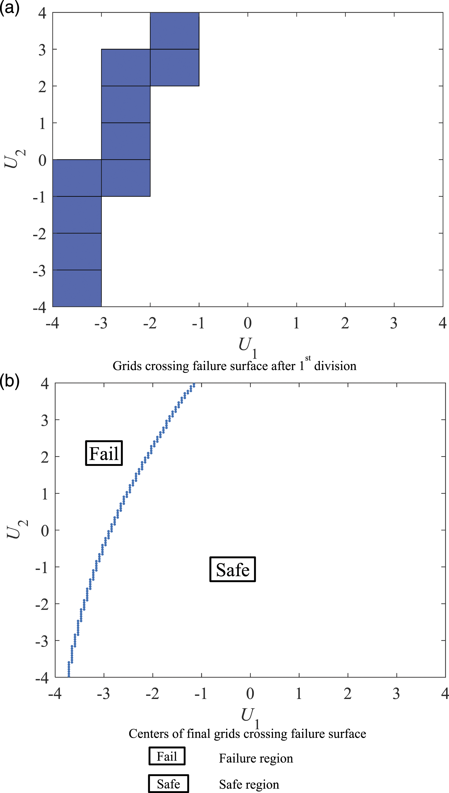
A parametric analysis using Method A is conducted on θs,th with this problem. The result is shown in Figure 8. It can be seen that for the case where the intersection point between a direction vector and failure surface is unique, if θs,th is too small (less than 10−2 in this case), the intersection points of a direction vector cannot be identified. As a result, the failure probability obtained is smaller than the true failure probability. If θs,th is larger than a threshold (10−2 in this case), accurate failure results can be obtained. Although a large θs,th (e.g., larger than 0.1) may result in a nonzero failure probability associated with a direction vector not crossing the failure surface, as these nonzero failure probabilities are very small, the influence of further increasing θs,th when it surpasses a threshold (10−2 in this case) on the overall failure probability considering all the direction vectors is minimal. Influence of θs,th on the failure probability associated with Example 2 using Method A.
Example 3: System reliability for a series system
The third example is associated with a series system consisting of four components. The equivalent performance function is expressed as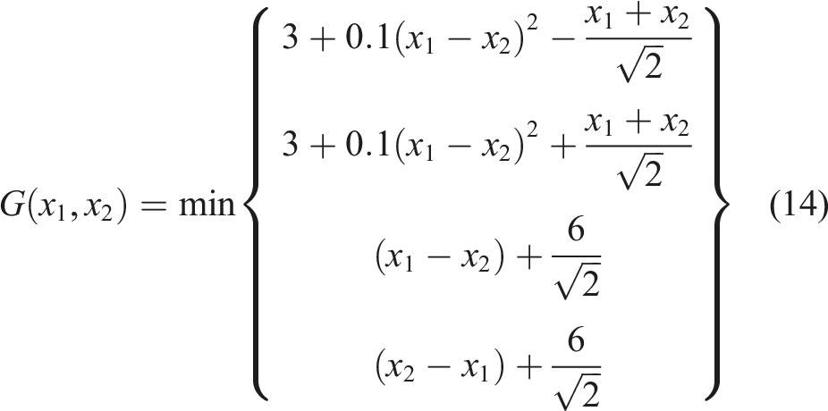
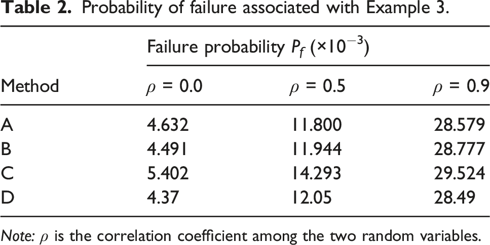
As indicated previously, for a series system, a direction vector can only intersect the failure surface once. The initial space and the values of parameter of interest are the same as those in Example 2. Scatter plots of the centers of the final grids crossing the failure surface associated with the three correlation cases in the U-space are shown in Figure 9, where failure and safe regions are indicated. It can be seen that correlation among random variables makes a difference in the shape of failure surface. The failure probabilities associated with four different methods are presented in Table 2. For the first correlation case (ρ = 0), the failure probabilities associated with Methods A and B match the result given in Sun et al., (2017). Considering all the three correlation cases, it can be seen that Methods A, B, and D give similar reliability analysis results. When the failure probability is not very small (larger than 10−4), using Monte Carlo simulation is expected to provide an accurate failure probability. Therefore, Methods A, B, and D can provide an accurate result for this problem. As near perfectly negative correlations exist among safety margins of some components in this series system, the failure probability obtained using Method C has a considerable error. It can be seen that the correlation among random variables in the performance function does not affect the applicability of the approach proposed herein to the system reliability analysis for series systems. Centers of final grids crossing the failure surface associated with different correlation coefficients ρ between the random variables in Example 3. (a) ρ = 0, (b) ρ = 0.5, (c) ρ = 0.9. Probability of failure associated with Example 3. Note: ρ is the correlation coefficient among the two random variables.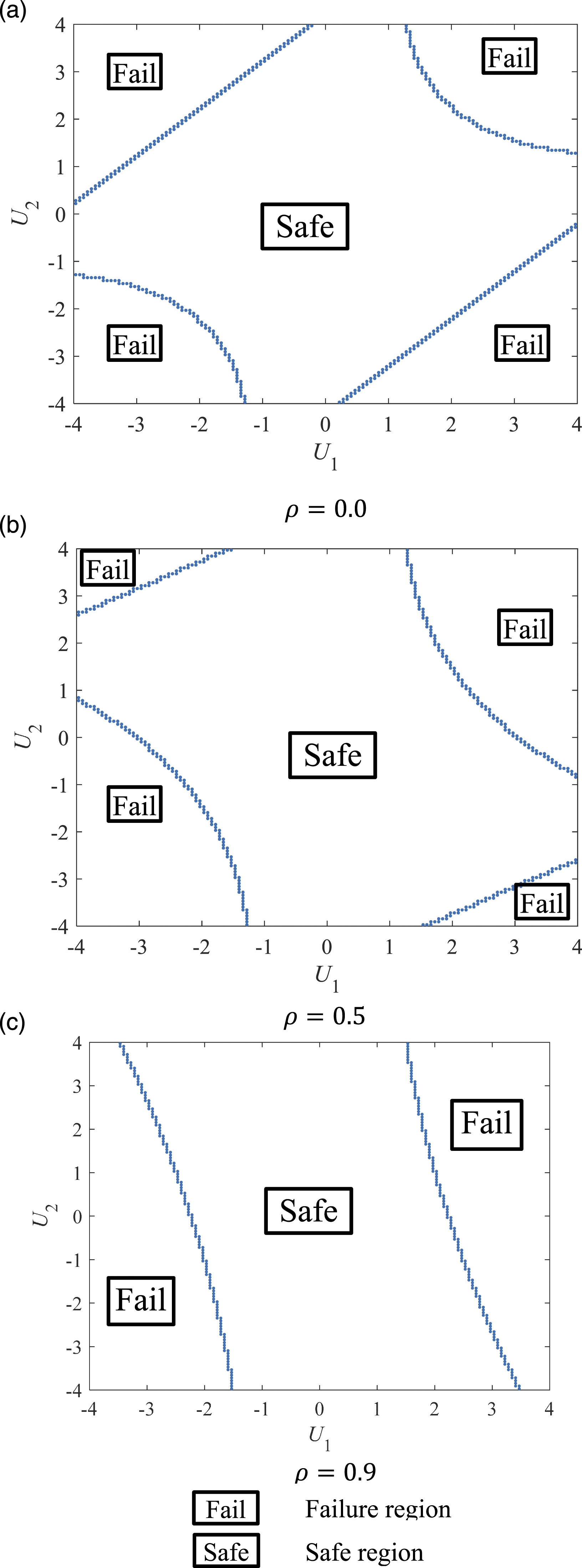
Example 4: System reliability for a parallel system
The fourth example is associated with a parallel system consisting of three components. The equivalent performance function is expressed as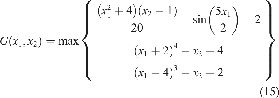
For the first and second correlation cases (i.e., ρ = 0 and = 0.5), the initial space is set as [−5, 5]×[−5, 5]. For the third correlation case (i.e., = 0.9), as the failure probability is very small, a larger initial space needs to be set to capture the failure surface. Through a trial-and-error process, the initial space for the third correlation case is determined as [−10, 10]×[−10, 10]. For all the three correlation cases, ϵ is set as 0.1. Taking the first correlation case as an example, three different values of N
r
, 1, 5, and 10, are set to investigate the influence of the number of generated samples on the failure probability. The centers of the final grids crossing the failure surface associated with these three N
r
values are shown in Figure 10. It can be seen in Figure 10(a) that a small N
r
may result in a failure to identify part of the failure surface. Therefore, for performance functions associated with an enclosed failure region, increasing N
r
may help capture the failure surface more accurately. When N
r
increases to a certain level, further increasing N
r
may not improve the characterization of failure surface significantly, as can be seen from Figure 10(b) and Figure 10(c) (in which the failure and safe regions are indicated). Centers of final grids crossing the failure surface associated with different numbers of generated samples in a grid N
r
in Example 4 with ρ = 0. (a) N
r
= 1, (b) N
r
= 5, (c) N
r
= 10.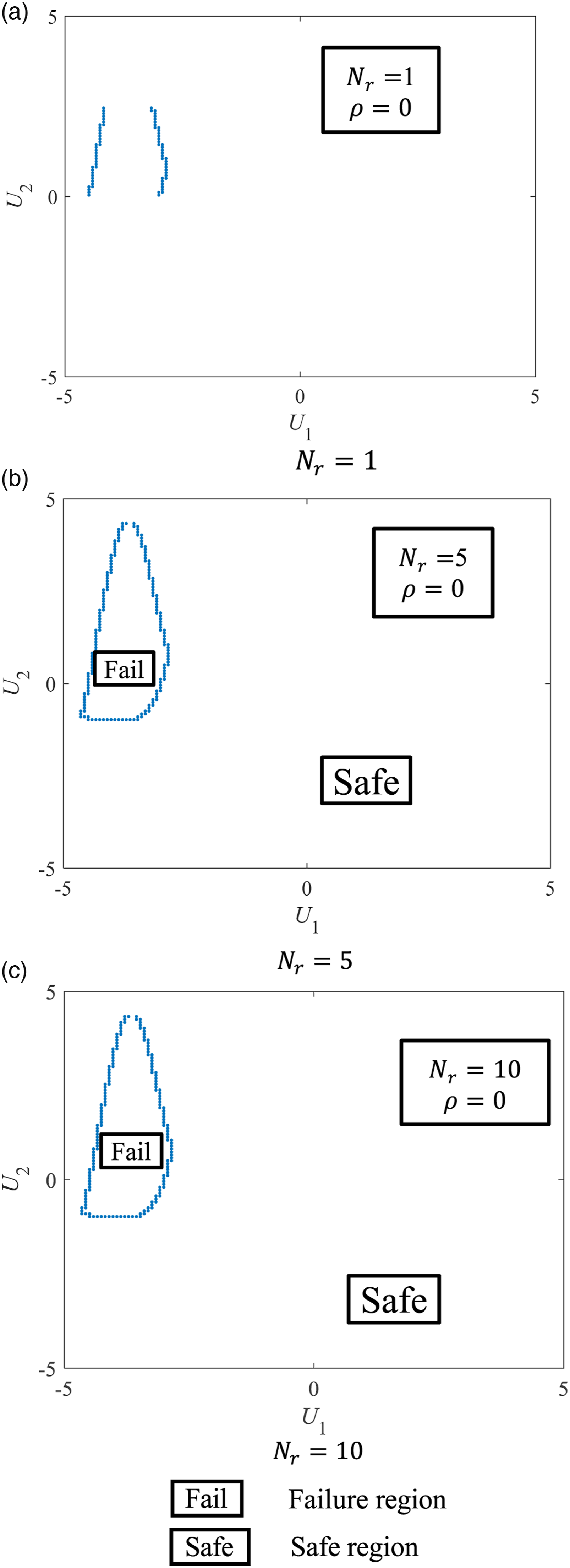
Probability of failure associated with Example 4.
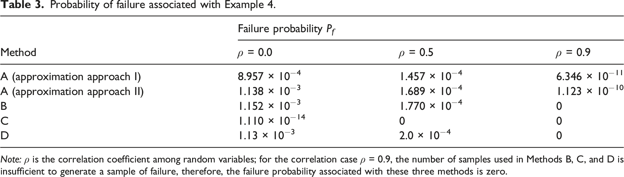
Note: ρ is the correlation coefficient among random variables; for the correlation case ρ = 0.9, the number of samples used in Methods B, C, and D is insufficient to generate a sample of failure, therefore, the failure probability associated with these three methods is zero.
A parametric analysis on θs,th in Method A is carried out for this problem associated with the first correlation case (ρ = 0). θ
th
is considered equal to θs,th and r
th
is equal to 10θ
th
. The relationship between failure probability given by Method A and θs,th is shown in Figure 11. It can be seen that a very small θs,th (smaller than 10−2 in this case) results in an underestimation of the failure probability while a large θs,th (larger than 0.05) results in an overestimation of the failure probability. Failure probabilities associated with a θs,th of 0.01 (the value used herein), is025, and 0.1 are indicated in Figure 11. The value of θs,th can be chosen from a range associated with the transition of the slope of the curve indicating the relationship between the failure probability and θs,th. In this case, θs,th between 0.01 and 0.025 is considered as acceptable. Influence of θs,th in Method A on the failure probability associated with Example 4 with ρ = 0.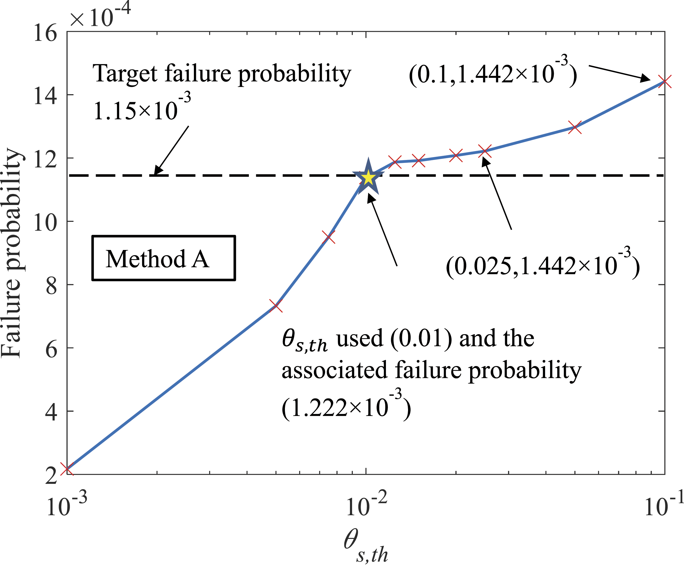
Example 5: Reliability analysis associated with multiple disconnected failure regions
For direction sample technique, the trickiest problem is the one associated with multiple disconnected failure regions (e.g., a performance function with multiple “holes” in its failure region). In this regard, reliability analysis associated with modified Rastrigin function (Echard et al., 2011) is investigated herein. The performance function is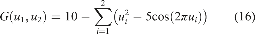
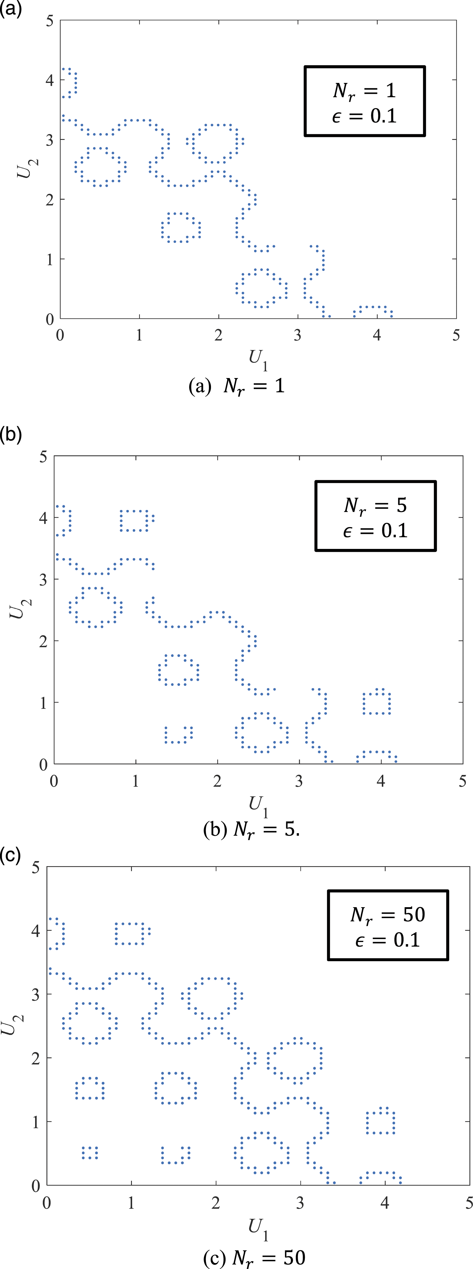
A 3D surface plot on the values of the performance function is shown in Figure 12. It can be seen that the function is associated with multiple local maxima and minima and intersects with the plane G(u1,u2) = 0 at multiple regions. As the modified Rastrigin function is symmetric with respect to both u1-axis and u2-axis, the failure surface in the first quadrant of the U-space is investigated and the direction sampling is conducted with the centers of grids in the first quadrant. The initial space is set as [0, 5]×[0, 5]. The centers of the final grids crossing the failure surface using N
r
= 1, 5, and 50 samples associated with ϵ = 0.1 are shown in Figure 13. It can be seen that to fully capture the failure surface with multiple small holes, a relatively large N
r
is needed. The influence of ϵ on the failure surface characterization is also investigated using this example. Using N
r
= 50, the centers of grids crossing the failure surface associated with ϵ = 0.05 and ϵ = 0.01 are shown in Figure 14(a) and 14(b), respectively. It can be seen that a smaller ϵ leads to a more accurate characterization of the failure surface. The safe region associated with this performance function is indicated in Figure 14(b). 3D surface plot of the modified Rastrigin function. Centers of final grids crossing the failure surface associated with different numbers of generated samples N
r
with an ϵ of 0.1 in Example 5. (a) N
r
= 1, (b) N
r
= 5, (c) N
r
= 50. Centers of final grids crossing the failure surface associated with different final grid sizes ϵ with a N
r
of 50 in Example 5. (a) ϵ = 0.05 , (b) ϵ = 0.01.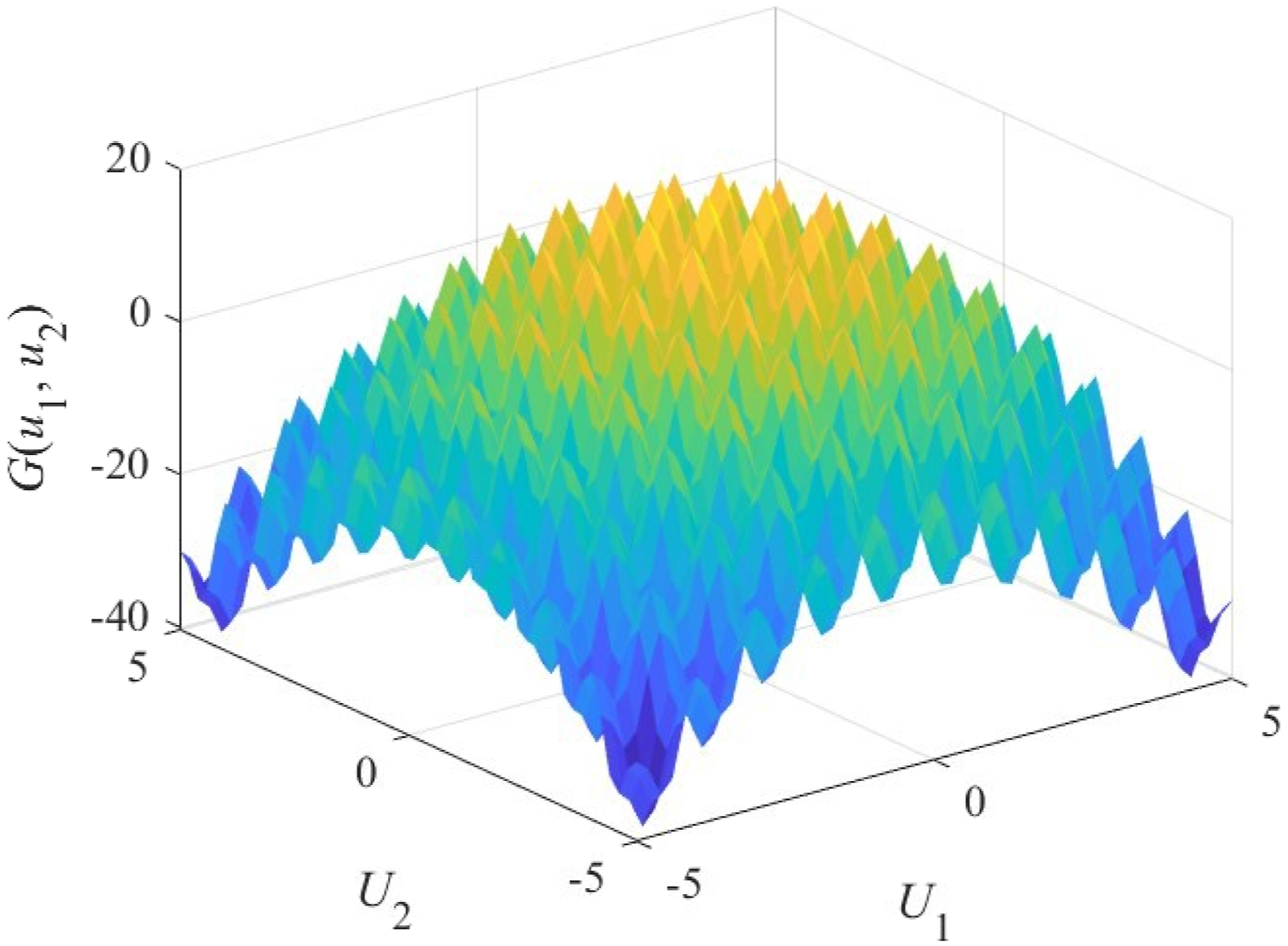
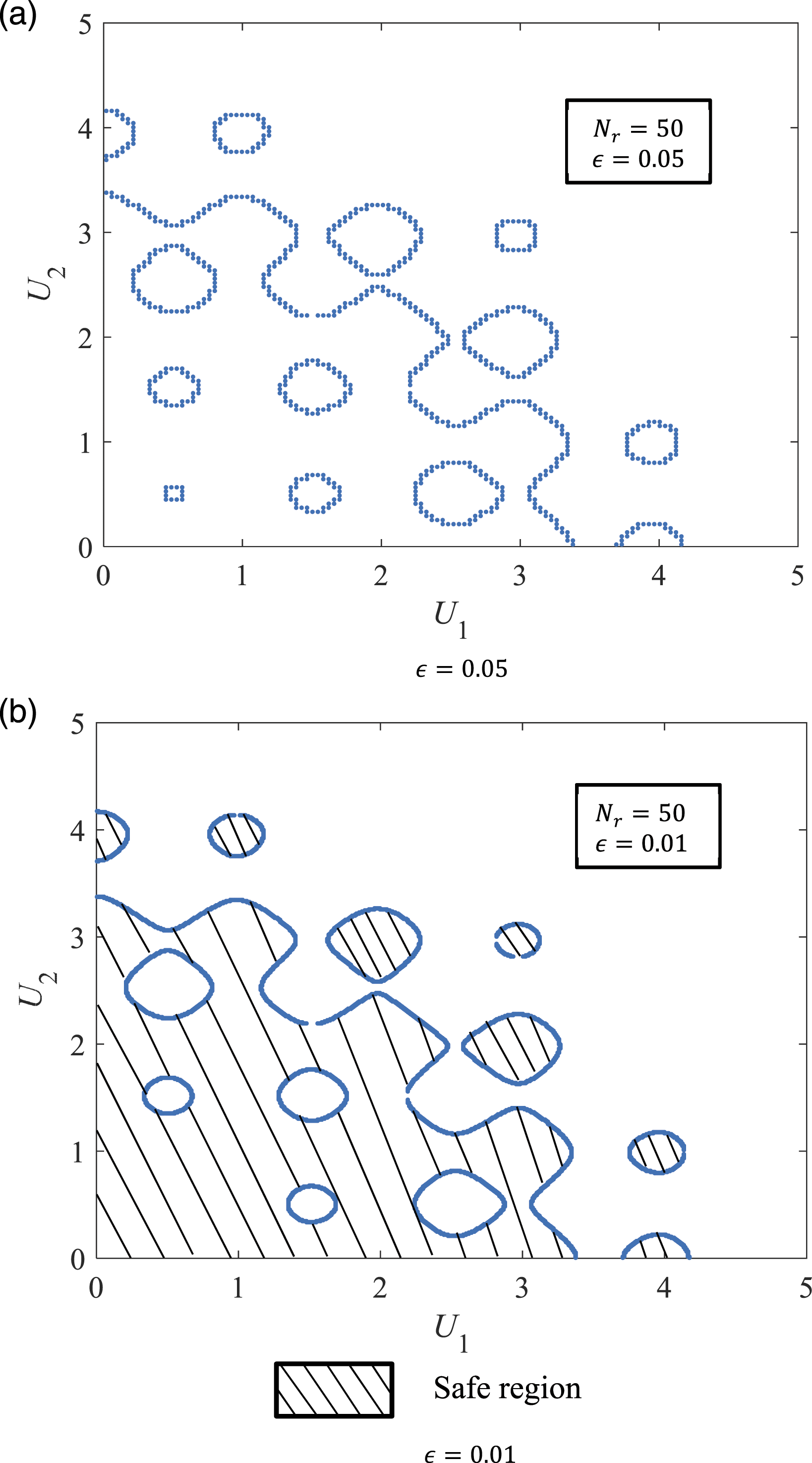
The centers of final grids crossing the failure surface associated with ϵ = 0.01 are used to obtain failure probabilities. θs,th and θs,th are both set as 0.005 while r th is set as 0.05. In this case the number of intersection points between a direction vector and the failure surface should be odd-numbered. For Method A, the failure probabilities associated with approximation approaches I and II are calculated as 5.490 × 10⁻² and 7.170 × 10⁻², respectively. The failure probabilities associated with Methods B, C, and D are calculated as 7.302 × 10⁻², 6.848 × 10⁻⁶, and 4.029 × 10⁻², respectively. For this problem, the results provided by Method A with approximation approach II and Method B are acceptable, while the results provided by Methods C and D are off the mark. It should be noted that although it is possible to obtain a satisfactory result using Method A, a relatively large N r and a relatively small ϵ are entailed, which implies a large computational cost. Therefore, for the reliability problem associated with multiple disconnected regions, using direction sampling may not be the optimal option.
Example 6: Reliability analysis integrating clustering techniques
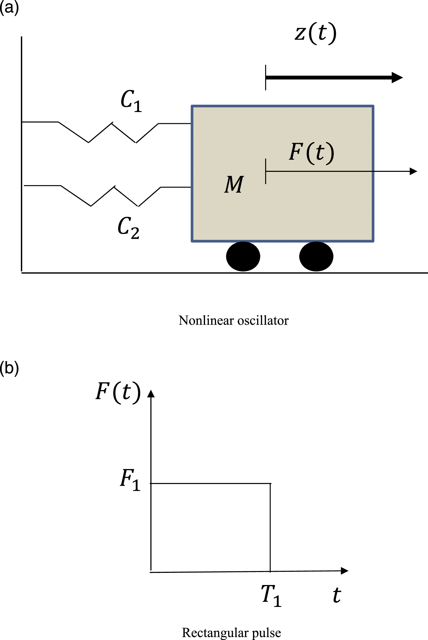
The integration of clustering techniques into the proposed approach is investigated herein. The example problem is associated with a nonlinear oscillator subjected to a rectangular pulse. An illustration of the oscillator and the external force is shown in Figure 15. This example problem was investigated in Zhang et al. (2021). The performance function is Illustration of a nonlinear oscillator subjected rectangular pulse (adapted from Zhang et al., (2021)). (a) Nonlinear oscillator. (b) Rectangular pulse.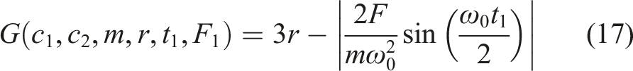
Although the performance function only involves six random variables, simulating the entire 6-dimensional failure surface with a fine discretization entails large memory so that a typical desktop with a memory of 16 gigabytes cannot be used. Therefore, clustering technique needs to be adopted in order to solve the problem using an ordinary desktop. As the focus of this example is to check the accuracy of Method A using clustering techniques, only the failure probability associated with Method A is calculated. For a failure probability as small as 9.1 × 10⁻⁶, the number of samples used in Methods B and D is insufficient. When absolute value is involved in a performance function, Method C also cannot provide an accurate failure probability.
The lower bound U l , upper bound U b , and the initial length the of grid in each dimension U int are set as −4, 4, and 2, respectively. The values of N r , ϵ, and θs,th are 1, 0.15, and 0.2, respectively. Clustering process is conducted for the grids crossing the failure surface after the first division (i.e., ϵ1=1). A total of 211 clusters are generated using K-means clustering algorithms. The number of grids within each cluster before further division is less than 10. For each generated direction samples, 12 clusters are selected based on the cross angles between the vector associated with the cluster centroid and the direction vector. To expedite the calculation process, it is assumed that if the minimum cross angle between the vector associated with the cluster centroid and the direction vector is larger than 0.3 radian, the direction vector does not intersect the failure surface and, therefore, the failure probability in that direction is zero. This is valid based on the cross angles between the vectors associated with the centroids of adjacent clusters. For the selected clusters, grid division and failure surface identification continue until U int is less than ϵ.
A total of 2 × 10⁴ samples is used to make sure the convergence of failure probability when only a part of failure surface is finely discretized. The relationship between number of samples and the failure probability is shown in Figure 16. It can be observed that for this example problem, the failure probability stabilizes when the number of samples reaches 104. The failure probability using 104 samples in Method A is 9.83 × 10⁻⁶. When the number of samples further increases, some small-scale fluctuations exist and the peak of the fluctuation is 1.02 × 10⁻⁵. As only part of grid on the failure surface is divided in a refined manner for each direction sample, error between the calculated result and the accurate result can be observed, However, even for the maximum value of the fluctuation when the number of samples is larger than 104, the relative error is within a reasonable range (about 12% in this case). Given the drastic reduction of the memory required and the acceleration of the computation speed, incentive exists on incorporating a clustering process in the entire lattice grid division process when the requirement on the accuracy of the reliability analysis is not very stringent. Relationship between number of samples and failure probability using Method A for Example 6.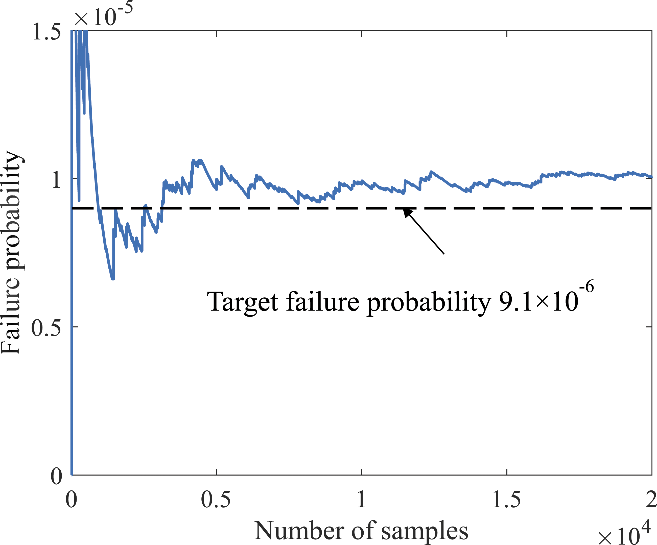
Conclusions
A novel approach to conduct reliability analysis is investigated herein. This approach is based on densely populate points on the failure surface and uses direction sampling to obtain failure probability. An iterative space division process is conducted to obtain small lattice grids crossing the failure surface. For a generated direction vector sample, the intersection points between it and the failure surface are selected among these centers of grids, thereby avoiding a root-searching process. The novelty of the proposed approach is enhanced by extending the scope of application to problems associated with multiple intersections between the direction vector and the failure surface. The applicability of the proposed approach can be further enhanced by using clustering techniques.
The following conclusions are drawn: 1. When the intersection between the direction vector and the failure surface is unique, the approach proposed herein can be adopted to solve the associated reliability problem. 2. When a direction vector intersects the failure surface multiple times, the proposed approach yields satisfactory results by using approximation methods. Furthermore, the proposed approach is applicable to reliability problems with connected failure regions. A significant advantage of the proposed approach is its ability to calculate small failure probabilities. 3. For reliability problems associated with multiple disconnected regions, it is still possible for the proposed approach to yield satisfactory results. However, as the number of samples increases and the final grid size decreases, the associated computational cost is expected to increase significantly. This is a limitation of the proposed approach. 4. For reliability problems with a high dimensionality, using clustering techniques can significantly reduce the computational cost. 5. It should be acknowledged that the curse of dimensionality is still the most daunting challenge for the proposed approach to achieve wide application. In addition to clustering techniques, directional importance sampling and dimension reduction techniques (Breitung, 2015) can also be used to enhance the applicability of the proposed approach.
Footnotes
Acknowledgments
The authors are grateful for the support provided by the National Science Foundation Award CMMI-1537926. The opinions and conclusions presented this paper are those of the authors and do not necessarily reflect the views of the sponsoring organization.
Declaration of conflicting interests
The author(s) declared no potential conflicts of interest with respect to the research, authorship, and/or publication of this article.
Funding
The author(s) disclosed receipt of the following financial support for the research, authorship, and/or publication of this article: This work was supported by the National Science Foundation Award CMMI-1537926.