Edge- and mid-span thermal-response signatures in continuous box-girder bridges

Abstract

Routine bridge-monitoring systems often provide much less information than research deployments. For routine monitoring of many in-service continuous box-girder bridges, the available record is limited to sparse temperature channels and one strain channel at each monitored section. This paper treats that sparse setting as the working condition and shows that such records still carry usable thermal-response information once lag, slow drift, and warming–cooling asymmetry are handled separately. Using 4 to 5 years of field data from six monitored sections of two cold-region prestressed concrete continuous box-girder bridges, branch-separated thermal response analysis (BSTRA) is developed to estimate a section-level thermal-response slope b. The procedure applies section-specific lag alignment, 12-h differencing, and separate warming/cooling branch fitting in differential space. Across the six monitored sections, the mean annual coefficient of variation of b falls from 105.8% in raw-space branch splitting to 6.0%, while the mean branch-fit R² increases from 0.182 to 0.738. After this stabilization, the edge spans show a cold-season-high, warm-season-low pattern. The two mid-span sections depart from this edge-span pattern: both show larger seasonal amplitudes, and one shows an opposite cold–warm seasonal direction. These results support the construction of span-region-specific monthly reference bands in the two bridge cases instead of a single pooled seasonal baseline.

Keywords

bridge structural health monitoring thermal response continuous box-girder bridge thermal-response signature section-region differentiation monitoring baseline lag-corrected differencing

Introduction

In structural health monitoring (SHM) of bridges, an instrumentation gap separates research practice from engineering practice. Research deployments often combine dense temperature fields, multi-axis strain rosettes, accelerometer arrays, and synchronized environmental sensing, which together support thermo-mechanical decomposition, finite-element updating, and digital-twin analysis (Brownjohn, 2007; Ko and Ni, 2005; Sohn et al., 2003; Farrar and Worden, 2007; Ni et al., 2005; Enckell et al., 2011; Xia et al., 2022; Miranda et al., 2025). These studies show that temperature is not a secondary background variable in bridge monitoring: it can dominate strain, displacement, modal properties, and the apparent baseline used for condition assessment. A related line of SHM research therefore treats environmental and operational variability as a central obstacle to damage detection and model interpretation (Peeters and De Roeck, 2001; Yan et al., 2005; Deraemaeker et al., 2008; Cross et al., 2011; Sohn, 2007). The much larger population of in-service bridges, including many expressway box-girder bridges in northeastern China, is monitored with a sparse routine configuration: typically one or two external-temperature channels, one or two internal-temperature channels, and a single strain channel per analyzed span. The records produced by such systems are routinely archived in management platforms, but they are not routinely used for structural interpretation, because the dense thermo-mechanical analysis methods developed on research bridges do not transfer directly to this sparse-monitoring setting.

Existing data-driven approaches do not directly fill this gap. Cointegration, Gaussian processes, neural networks, and LSTMs can all predict monitored strain or deflection with good accuracy when thermal forcing is included (Peeters and De Roeck, 2001; Cross et al., 2011; Kromanis and Kripakaran, 2017; Radicioni et al., 2025; Yue et al., 2022; Zhou et al., 2024; Gong et al., 2024; Miranda et al., 2025). Prediction accuracy, however, is not the same thing as a span-comparable descriptor. The fitted mappings depend on the specific bridge, sensor placement, training period, and feature set, so the resulting models are not portable across spans or across years in a form that engineers can compare month by month. Cointegration and statistical detrending pursue a different goal: they remove the temperature-driven component so that residuals can be analyzed for damage. This is useful, but it discards the slope information that thermal-response interpretation needs. Direct temperature–strain regression keeps that information in principle. Applied to multi-year cold-region records, however, it collapses the warming–cooling hysteresis loop into a single coefficient. The fitted value is then dominated by slow drift and inter-annual leverage, not by the structural response we want to read.

For continuous box-girder bridges in cold regions, the difficulty is more acute. Annual external-temperature ranges of 60°C and above produce strong seasonal forcing and pronounced through-section gradients, and the temperature–strain point cloud measured at the same span no longer collapses onto a single band when records from different years are overlaid (Sohn, 2007; Xia et al., 2012; Hu et al., 2022; Yang et al., 2024; Liu et al., 2019; Zhang et al., 2021; Zhou et al., 2025; Zhang et al., 2026). Several effects act at once. The strain response lags ambient temperature, the warming and cooling halves of a daily cycle do not retrace the same path, and slower processes such as creep, shrinkage, and bearing evolution introduce non-stationary drift over years. A descriptor read straight off the raw point cloud absorbs all of these. The opposite move—filtering temperature out of the record—solves the mixing problem but discards the slope itself.

The sparse routine configuration is therefore treated here as a workable monitoring condition rather than as a failed dense-instrumentation case. Sparse records do carry section-level thermal-response information, but reading it requires that the three effects above be addressed individually before any slope is fitted. This idea is packaged into a fixed analysis protocol, branch-separated thermal response analysis (BSTRA). BSTRA does not introduce a new estimation theory. Cross-correlation lag identification, finite differencing, and branch-wise linear regression are all standard tools. The point is the combination and the order: lag calibration first, 12-h differencing second, warming/cooling branch separation third, with all settings fixed in advance and applied uniformly across monitored sections.

Once b is repeatable enough to compare across spans, a second pattern in the data becomes readable. Edge spans and mid-spans of continuous box-girder bridges do not share one seasonal baseline. The extracted signatures show that the section region is associated with the seasonal pattern, even though the present dataset cannot identify which local mechanism is responsible. In what follows we use thermal-response signature for the seasonal pattern of b at a given span, and treat the edge–mid-span gap as the main engineering finding.

Earlier long-term bridge studies have used combinations of temperature, strain, displacement, and modal-response channels to interpret seasonal behavior (Cardini and DeWolf, 2009; Liu et al., 2009; Cury and Cremona, 2012; Meixedo et al., 2021; Sawicki and Bruhwiler, 2020; Le and Nishio, 2015; Nepomuceno et al., 2022; Zhu et al., 2022), and recent work has increasingly combined monitoring data with regression, machine learning, or numerical simulation to compensate or predict temperature-driven response (Kromanis and Kripakaran, 2017; Ren et al., 2022; Yue et al., 2022; Zhou et al., 2024; Gong et al., 2024; Miranda et al., 2025). Taken together, the literature establishes three points: temperature effects are often dominant, environmental compensation is necessary before structural interpretation, and bridge-specific case studies are valuable for understanding field behavior. What remains less developed is a fixed, low-instrumentation protocol that keeps the temperature-response slope itself as the target quantity and then compares that quantity across structural regions and years.

Manuscript framework

Figure 1 summarizes the role of BSTRA in the manuscript. The study first defines the sparse routine monitoring setting and the two bridge cases, while the detailed Bridge A and Bridge B inventory is intentionally deferred to the next section. It then applies the same analysis chain to every monitored section: lag calibration, 12-h differencing, warming/cooling branch separation, and monthly or yearly extraction of the thermal-response slope b. The results are evaluated in two steps. First, baseline and ablation comparisons test whether the protocol makes b more stable than direct raw-space regression. Second, the stabilized b values are compared across edge-span and mid-span sections to determine whether one seasonal baseline is adequate for the monitored continuous-girder units. Used this way on six monitored sections from two cold-region prestressed concrete continuous box-girder bridges, each with four to 5 years of data, the resulting section-level slope b has an annual coefficient of variation of about 6%, compared with more than 100% from the same branch-splitting step applied directly in raw space. The four edge spans show monthly b higher in the cold season and lower in the warm season, whereas the two mid-spans depart from that pattern in different ways.

Figure 1.

Conceptual overview of the BSTRA framework.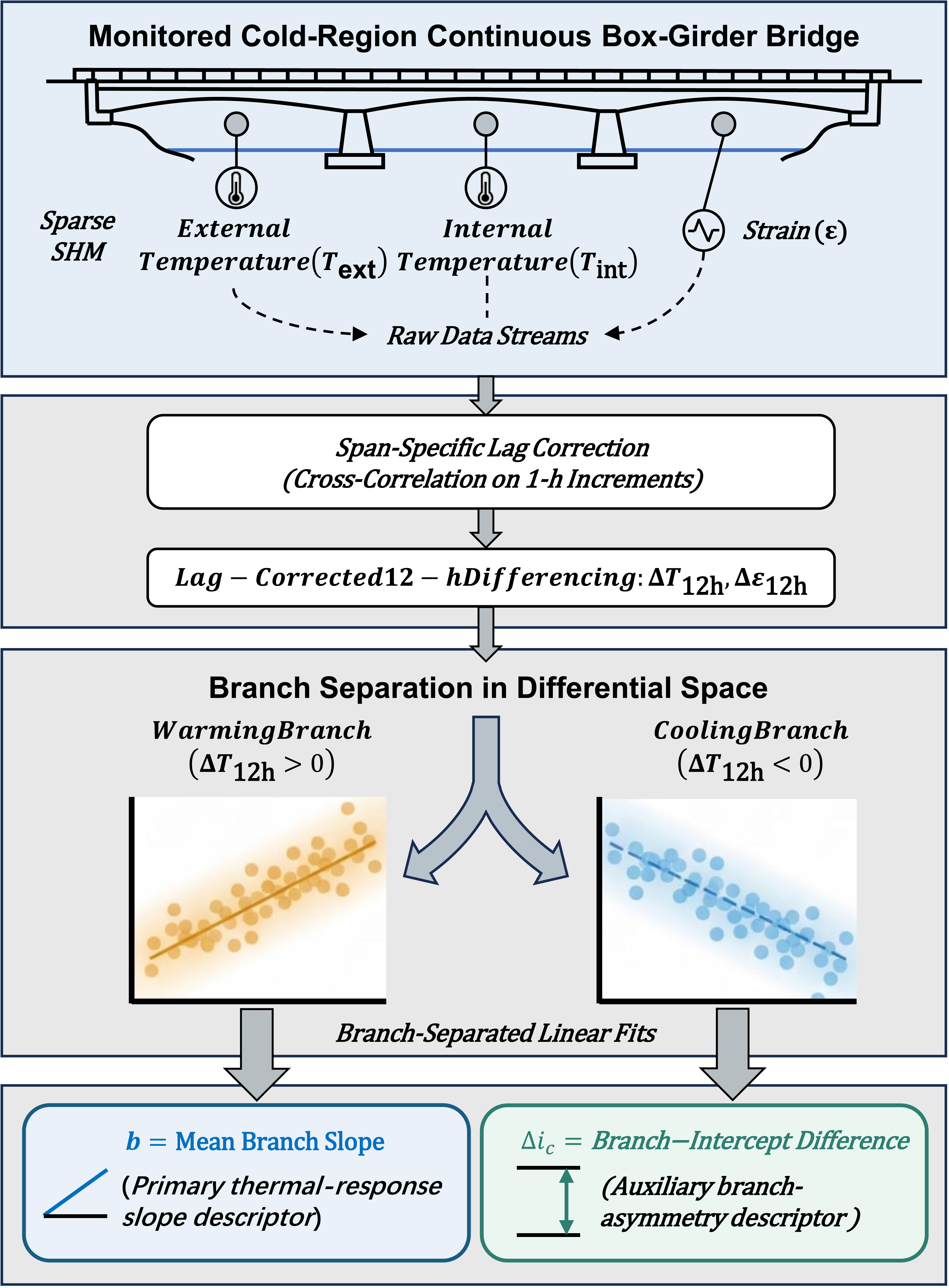

The remainder of the paper follows this framework. Section “Bridge Cases and Monitoring Data” describes the two monitored bridges and their data quality. Section “Methodology” formalizes the BSTRA protocol and the baseline and ablation comparisons used later. Section “Results” reports the cross-span performance of BSTRA, the annual stability of b, the monthly seasonality, and the edge–mid-span contrast. Section “Discussion” interprets b as a section-level thermal-response slope, develops the thermal-response signature view, and clarifies the role of the auxiliary asymmetry descriptor. Section “Conclusions” summarizes the protocol contribution and the section-region finding, and outlines the implications for monitoring practice on bridges that operate with similar routine temperature–strain monitoring records.

Bridge cases and monitoring data

Bridge inventory and structural context

Two prestressed concrete continuous box-girder bridges in Liaoning Province were selected as case studies. Bridge A is an expressway bridge analyzed here over 2018–2021. Bridge B is also an expressway bridge, analyzed here over 2019–2023, with the monitored bridge crossing a railway corridor. Both bridges are three-span continuous box-girder systems with one mid-span section and two edge spans included in the present analysis. Here and below, edge span and mid span are span-region terms: all analyzed sections are located at the midsection of their respective spans, with S2/S9 located in the middle span and the remaining sections located in edge spans. The monitored sections are denoted S1–S3 for Bridge A and S8–S10 for Bridge B. Their basic monitoring scope is summarized in Table 1.

Table 1.

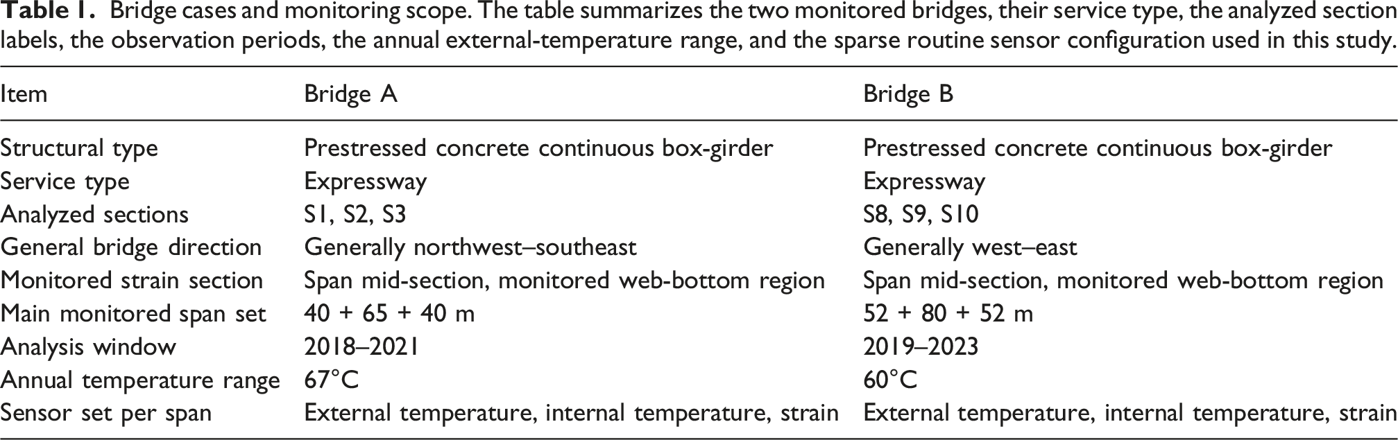
Bridge cases and monitoring scope. The table summarizes the two monitored bridges, their service type, the analyzed section labels, the observation periods, the annual external-temperature range, and the sparse routine sensor configuration used in this study.

Item	Bridge A	Bridge B
Structural type	Prestressed concrete continuous box-girder	Prestressed concrete continuous box-girder
Service type	Expressway	Expressway
Analyzed sections	S1, S2, S3	S8, S9, S10
General bridge direction	Generally northwest–southeast	Generally west–east
Monitored strain section	Span mid-section, monitored web-bottom region	Span mid-section, monitored web-bottom region
Main monitored span set	40 + 65 + 40 m	52 + 80 + 52 m
Analysis window	2018–2021	2019–2023
Annual temperature range	67°C	60°C
Sensor set per span	External temperature, internal temperature, strain	External temperature, internal temperature, strain

Site photographs of the two monitored bridges are shown in Figure 2. These photographs are included to document the bridge context and to distinguish the two field cases before the monitoring records are discussed.

Figure 2.

Site photographs of the two monitored bridge units. Panel (a) shows Bridge A and panel (b) shows Bridge B.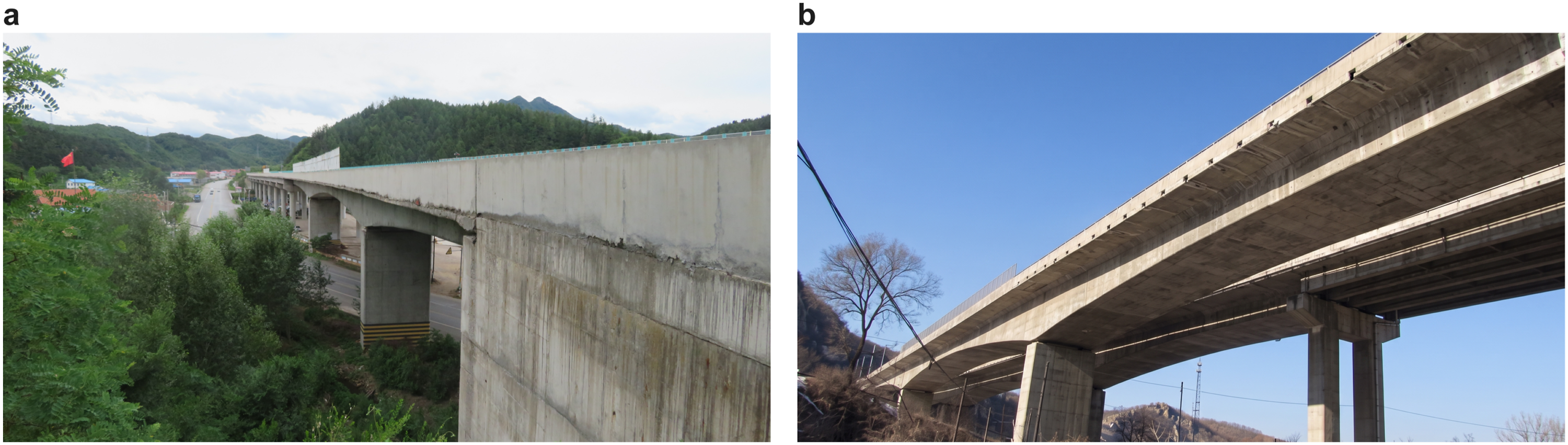

Both bridges are located in a cold-region environment with strong seasonal thermal forcing. The annual external-temperature range reaches 67°C for Bridge A and 60°C for Bridge B. The monitored three-span sets are 40 + 65 + 40m for Bridge A and 52 + 80 + 52m for Bridge B. Bridge A is generally northwest–southeast oriented, and Bridge B is generally west–east oriented. The routine strain and internal-temperature channels are located in the monitored web-bottom regions shown schematically in Figure 3, and the beam-exterior temperature channel is indicated separately outside the box-girder section. Both bridges carry expressway traffic, although their detailed site surroundings are not identical. The pair provides a useful comparison under similar bridge form with different operating surroundings, although the present dataset is intended for within-bridge and cross-span comparison, not for broad generalization across bridge types. The corresponding cross-section and broad orientation context is summarized in Figure 3.

Figure 3.

Monitoring-layout schematic for the analyzed bridge units. Panel (a) shows Bridge A (40 + 65 + 40 m) and panel (b) shows Bridge B (52 + 80 + 52 m). In each panel, the upper drawing shows the longitudinal profile of the monitored three-span unit, where S1–S3 or S8–S10 mark the monitored sections at the midsections of the three spans, together with the support-line labels (A0/P1–P3 or P7–P10) and the route-axis directions. The lower drawing shows the corresponding box-girder cross section, the beam-exterior temperature channel (T_ext) indicated schematically outside the box-girder section, the monitored strain/internal-temperature point at the web-bottom region, and the nominal neutral axis (dashed line). B and H denote the nominal top width and section depth. The vertical dimensions beside each cross section give the available elevation of the strain/internal-temperature point above the section bottom and its distance to the nominal neutral axis; parenthesized values correspond to the main-span midsection. The T_ext marker is schematic, and the schematics are not to scale.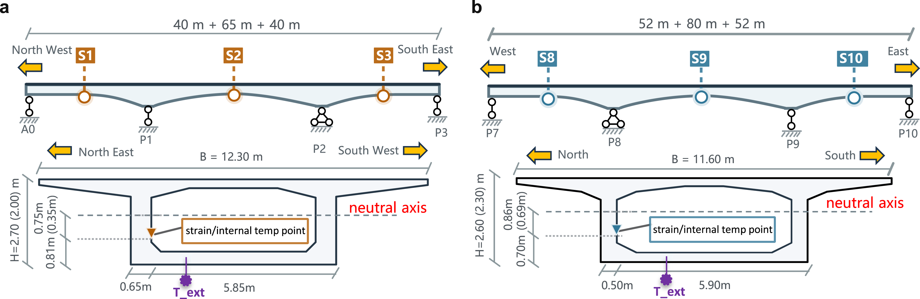

Monitoring System, Sensors, and Data Coverage

Each analyzed section contains one external-temperature measurement, one internal-temperature measurement, and one strain measurement at the bottom region of the web near the analyzed section. The raw channel metadata locate the Bridge A and Bridge B strain and internal-temperature channels in the web-bottom region of the span mid-section. The archived monitoring metadata identify the strain channel by span and web-bottom location, and Figure 3 reports both the schematically indicated beam-exterior temperature channel and the strain/internal-temperature position, together with the available vertical and transverse coordinates of the latter relative to the cross-section geometry and nominal neutral axis. The sensor position is therefore treated as section-specific and fixed for each span, and the interpretation below is made at the level of the monitored section rather than as a neutral-axis-independent material response. This sensor layout is already available in the multi-year bridge observation system, and it is close to the instrumentation level that is realistic for repeated bridge-level deployment. The same sparse routine configuration is available for all analyzed sections in both bridges. In the present analysis, the external-temperature channel is used as the common excitation variable so that the span-to-span comparison remains uniform under a sparse-monitoring workflow. That choice favors cross-span consistency and deployment simplicity over a full thermal-field description. The internal-temperature channel is retained as auxiliary context for sensor interpretation and future model refinement, but it is not used in the branch-regression equations reported here. Similar combinations of temperature and strain channels have been used in long-term bridge observations to interpret thermal response without requiring dense instrumentation at every section (Le and Nishio, 2015; Sawicki and Bruhwiler, 2020; Nepomuceno et al., 2022; Zhu et al., 2022; Miranda et al., 2025).

The Bridge A analysis window covers 4 years, from January 2018 to December 2021. The Bridge B analysis window covers 5 years, from January 2019 to December 2023. Longer raw monitoring records are available for both bridges, but only the retained quality-controlled intervals above are used for year-wise and month-wise comparison. Partial-year records are not mixed with full-year records, and heavily incomplete periods are not given equal weight. Figure 4 shows representative raw temperature and strain records from the two bridges. The external-temperature records indicate sustained sub-zero winter conditions and large seasonal reversals in both bridges. The strain records show clear seasonal oscillation superimposed on slower long-term drift. In Figure 4(b) and (e), the apparent long-term increase in compressive-direction strain is most plausibly read as a slow web-bottom shortening or baseline component superimposed on the seasonal cycles. For prestressed concrete box girders, sustained compression, prestress effects, concrete creep, and shrinkage can accumulate strain in the compressive direction over multi-year records; evolution of restraint conditions may also shift the measured baseline. This interpretation is consistent with long-term prestressed-concrete bridge monitoring evidence: temperature-compensated concrete strain in the Streicker Bridge increased in compression and then stabilized, distributed measurements in the Nine Wells Bridge were governed by prestress, creep, and shrinkage, and lower-web concrete gauges in the Westend Bridge showed persistent negative strain baselines (Hu et al., 2018; Abdel-Jaber and Glisic, 2019; Webb et al., 2017). These references are used to support the presence of mixed low-frequency concrete-strain baselines, not to imply that all bridges show the same trend direction. In the present sparse records, seasonal thermal-baseline changes and possible sensor or instrument baseline drift may also contribute, so the raw trend is not attributed to one uniquely identified mechanism. This slow component is one reason why BSTRA estimates the seasonal thermal-response slope from lag-corrected 12-h increments rather than from the raw multi-year trend. When temperature and strain are plotted directly against each other, the point clouds from different years do not collapse onto a single band; this is the main reason for introducing the branch-based analysis developed later.

Figure 4.

Representative raw monitoring data from the two bridge cases.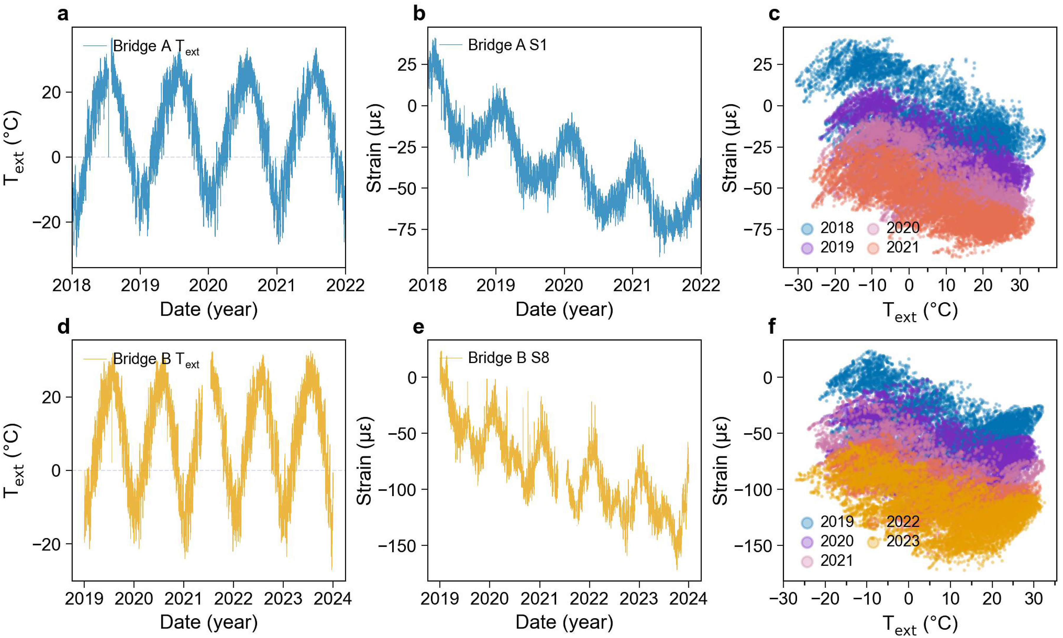

Data quality issues and analysis windows

For Bridge A, a common 4-year window (2018–2021) is adopted for all three spans. The 2022 record is excluded because its data loss is severe, especially in the mid-span section S2 where the missingness reaches 54% and is concentrated mainly in the second half of the year, which would distort both annual and monthly summaries if retained. Within the retained Bridge A window, the S2 lag check remains centered at 7 h, whereas the edge spans use lags of 3-4 h. Bridge B, by contrast, retains its full 2019–2023 5-year window because the year-wise and month-wise data coverage remains adequate for the comparative analyses used here.

The filtering keeps only those spans and years for which the lag-calibration behavior is internally consistent and the valid data coverage is sufficient for both branch fitting and month-wise comparison. The same rule also motivates the bridge-level analysis windows reported above: years with severe missingness or partial-year coverage are not mixed indiscriminately into the main comparative baseline. For the remaining spans, the calibrated lag remains stable across the observation period, which supports the use of span-specific fixed lags in the downstream analysis. In the monthly figures, the plotted monthly means and their inter-annual standard-deviation error bars are computed only from the retained valid years for each calendar month, so months with heavy missingness do not contribute to the displayed summaries.

Methodology

Lag calibration

The first step is to account for the thermal inertia between ambient temperature variation and measured strain response. For each span, the lag is estimated from the cross-correlation between the hourly temperature increment and the hourly strain increment. Cross-correlation-based lag identification has been widely used in temperature-response studies where phase mismatch between excitation and response must be reduced before regression or compensation (Cao et al., 2011; Zhou and Sun, 2019; Yang et al., 2024). Let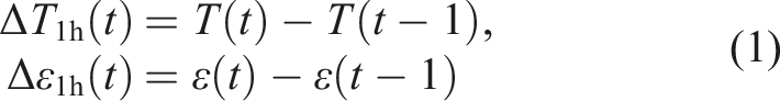

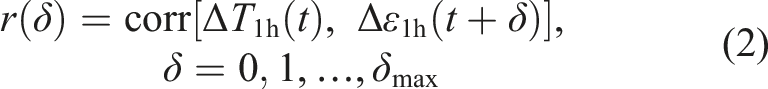
\begin{aligned} Δ T_{1 h} (t) & = T (t) - T (t - 1), \\ Δ ε_{1 h} (t) & = ε (t) - ε (t - 1) \end{aligned}

(1)

where T is the external temperature and ɛ is the monitored strain. The external-temperature channel is fixed as the excitation proxy for all reported branch regressions so that the workflow remains comparable across spans and uses the sparse routine sensor configuration available on both bridges. Internal temperature is retained as auxiliary thermal context and for sensitivity checking, but it is not used to choose a different excitation channel span by span. The lag-dependent correlation is then evaluated over a finite lag range,

\begin{aligned} r (δ) & = c o r r [Δ T_{1 h} (t), Δ ε_{1 h} (t + δ)], \\ δ = 0,1, \dots, δ_{\max} \end{aligned}

(2)

and the selected lag is

δ^{*} = \arg \max_{δ} | r (δ) |

(3)

with δ_max = 16 h in the present study. The procedure is carried out span by span, and the resulting lag is then kept fixed for that span in all yearly, monthly, and baseline calculations. The lag is not re-tuned against the final branch-fit R² or against the inter-annual stability of b. Yearly recalculations are used only to confirm that the selected lag remains stable over time.

The cross-correlation peak is used here for alignment, not as an estimate of any physical time constant. The peak position reflects the combined chain by which air temperature reaches the strain sensor: convective exchange at the surface, heat conduction through the section, and the resulting section-level deformation at the sensor location. The procedure does not separate these contributions, and is not intended to. What matters for the downstream analysis is that the same alignment is applied to all retained (T, ɛ) pairs at a given monitored section. We tested whether the downstream descriptor is sensitive to fine-scale lag choice by repeating the indicator extraction with δ* ±1 h at each analyzed section. The annual coefficient of variation of b stayed within 2.6%–11.6% across the perturbed cases, comparable to the 3.1%–10.9% range at the calibrated lag. The mean level of annual b is more sensitive to lag perturbation than its inter-annual stability—the largest mean-b shift across the six monitored sections is 13.7%, and shifts are smaller at sections whose calibrated lag is larger relative to the perturbation step. The pattern supports two practical points: the CCF-selected lag is a non-arbitrary calibration choice, and BSTRA should not be applied to records where that lag has not been calibrated. The section-specific CCF curves and year-wise lag checks are shown in Figure 5.

Figure 5.

Cross-correlation-based lag calibration for the analyzed sections.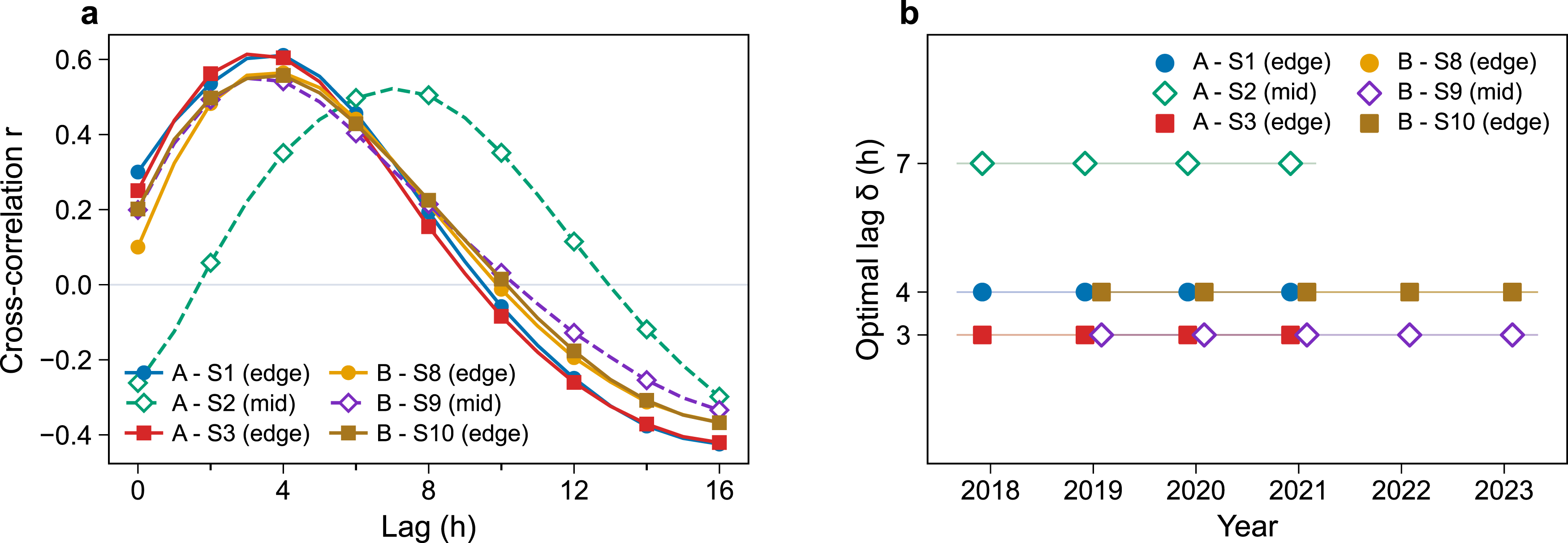

In the present study, BSTRA is developed and evaluated for bridge strain monitoring. Its transfer to other structural monitoring settings would require separate validation, especially where the dominant excitation, response lag, and sensor configuration differ from those studied here.

Lag-corrected 12 h differencing

After lag selection, the temperature and strain series are transformed into a lag-corrected 12-h differential space. The differencing operator x(t + τ) − x(t) has frequency response magnitude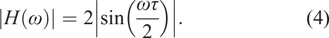

| H (ω) | = 2 |\sin (\frac{ω τ}{2})| .

(4)

For the dominant daily cycle, ω₀ = 2π/24 h⁻¹, the magnitude in equation (4) reduces to |H(ω₀)| = 2| sin(πτ/24)|. This expression equals 1.00 at τ = 6 h, peaks at 2.00 at τ = 12 h, returns to 1.00 at τ = 18 h, and falls to 0 at τ = 24 h. A 12-h window preserves the daily warming–cooling reversal at maximum amplitude, while a 24-h window suppresses it entirely; substantially shorter windows retain the daily cycle but at reduced amplitude and are also more exposed to short-term fluctuations and residual intra-day irregularity. The same window is fixed a priori for all spans as a common analysis baseline, not optimized separately for each bridge or span and not claimed to be globally optimal for every climate. The supplementary window-sensitivity check follows this analytical pattern: branch-fit quality and seasonal b amplitude rise from τ = 6 h to τ = 12 h, decline gradually toward τ = 18 h, and drop sharply at τ = 24 h on representative edge-span and mid-span sections. The mean annual b shifts by less than about 10% between τ = 6 and τ = 18 h relative to the τ = 12 h baseline. The 12-h window is not an arbitrary convenience. It is the value at which the differencing operator most strongly amplifies the dominant daily cycle while suppressing slower drift. The empirical behavior of b across the tested windows matches this frequency-response argument.

For a differencing window τ = 12 h and span-specific lag δ*,

Δ T_{12 h} (t) = T (t + τ) - T (t)

(5)

Δ ε_{12 h} (t) = ε (t + τ + δ^{*}) - ε (t + δ^{*})

(6)

Here a positive δ* means that the strain response lags behind the temperature variation, so the strain series is shifted forward by δ* hours when constructing the lag-corrected difference. Physically, such lag is plausible because the monitored web-bottom strain does not react to air temperature instantaneously: heat must first propagate through the girder section, internal temperature gradients must evolve, and the resulting sectional deformation must develop at the sensor location. The longer lag observed at Bridge A S2 is interpreted here as a slower effective thermal response at that monitored section, not as a separately identified mechanism. Only pairs with finite values and sufficiently large temperature change are retained. In this study, data are kept only when |ΔT_12h| ≥ 1.0°C. This threshold is above the temperature-resolution scale of the monitoring records and is used as a fixed weak-excitation filter to avoid fitting branch slopes from near-zero temperature changes, where regression leverage and sensor noise become disproportionately important. It is not adjusted by section or by year. Threshold checks at 0.5, 1.0, and 1.5°C changed the mean annual b by at most 0.17% relative to the 1.0°C baseline, with annual b coefficients of variation remaining within 3.0%–10.9% across the six monitored sections. We kept 1.0°C as a conservative baseline; it is not an optimized tuning value. Within the tested range, the descriptor changes very little with the threshold choice. In these data, the 12-h differencing suppresses slow drift enough for the warming and cooling branches to separate in the differential space. Differential and regression-based treatments are common in long-term bridge monitoring; they help suppress slow-trend contamination and make the records easier to interpret (Farreras-Alcover et al., 2015; Kromanis and Kripakaran, 2017; Zhu et al., 2018; Ren et al., 2022). The differenced pairs are then analyzed month by month and year by year.

Branch-separated regression and indicator definition

The differenced samples are split into warming and cooling branches according to the sign of ΔT_12h. Samples with ΔT_12h > 0 form the warming branch, and samples with ΔT_12h < 0 form the cooling branch. Here, warming and cooling refer to the within-day temperature increment captured by the 12-h differencing operator, not to seasonal warm or cold periods; both branches contain samples from all calendar months. For each branch k ∈ {w, c}, a linear regression with intercept is fitted,

Δ ε_{12 h} = a_{k} Δ T_{12 h} + i c_{k}

(7)

where a_k is the branch slope and ic_k is the branch intercept. The primary branch-separated slope descriptor is then defined as

b = \frac{a_{w} + a_{c}}{2}

(8)

Δ i c = | i c_{w} - i c_{c} |

(9)

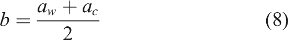
In this paper, b is used as a repeatable section-level thermal-response descriptor for the specific monitored section and sensor location. Mechanically, it is the apparent increment of measured web-bottom strain per unit 12-h external-temperature increment after lag alignment and slow-drift suppression. Operationally, for example, b = 1.4 μɛ/°C means that a 1°C increase in the lag-aligned 12-h external-temperature increment is associated with about 1.4 μɛ increase in the measured web-bottom strain at that specific gauge. A larger absolute value of b means that the monitored gauge strain changes more strongly for the same short-window thermal excitation, while the sign reflects the local strain-orientation convention and the combined axial–bending response at that gauge. The most useful mechanical intuition is that b folds together three structural effects: effective thermal expansion or contraction of the monitored section, thermal curvature produced by through-section temperature gradients, and longitudinal compatibility and restraint imposed by the continuous girder and bearings. Temperature-dependent stiffness of the concrete and surfacing and the sensor coordinates relative to the local neutral axis modulate this combined response; a strain gauge closer to a bending-sensitive region would not read the same thermal slope as a gauge placed elsewhere in the section. Thus, b is an empirical tangent-like monitoring slope, not a calibrated stiffness modulus, an independent material parameter, or a direct coefficient of thermal expansion. The average of the two branch slopes is used because it tracks the central response level while keeping warming and cooling samples in separate fits, which makes b comparable across spans even when a_w and a_c differ slightly. The intercept gap Δic is kept only as an auxiliary branch-asymmetry descriptor, defined as the unsigned difference |ic_w − ic_c| at ΔT_12h = 0. Δic is estimated from two often-overlapping branch fits and is treated here as exploratory information, not as a calibrated diagnostic. A monthly Δic estimate is retained only when both branches contain at least 30 valid samples after filtering; yearly estimates are computed from the full retained yearly records for each span. The branch-separation construction and the forward/return path analogy are illustrated in Figure 6. The forward path represents the daytime warming portion of the daily thermal cycle, during which increasing external temperature drives heat transfer into the box-girder section and develops through-section thermal gradients. The resulting web-bottom strain response lags behind the temperature change and is shaped by continuity and bearing restraint. The return path represents the cooling portion, during which the section releases heat and the restrained strain response does not necessarily retrace the warming path.

Figure 6.

Branch separation in the lag-corrected differential space. In panel (b), the forward and return paths are a normalized schematic analogy for the two directional portions of a daily thermal cycle at the monitored box-girder section: the forward path corresponds to the 12-h warming branch, and the return path corresponds to the 12-h cooling branch. The panel illustrates path dependence only; it is not measured temperature–strain data and is not a calibrated friction, bearing, or material model.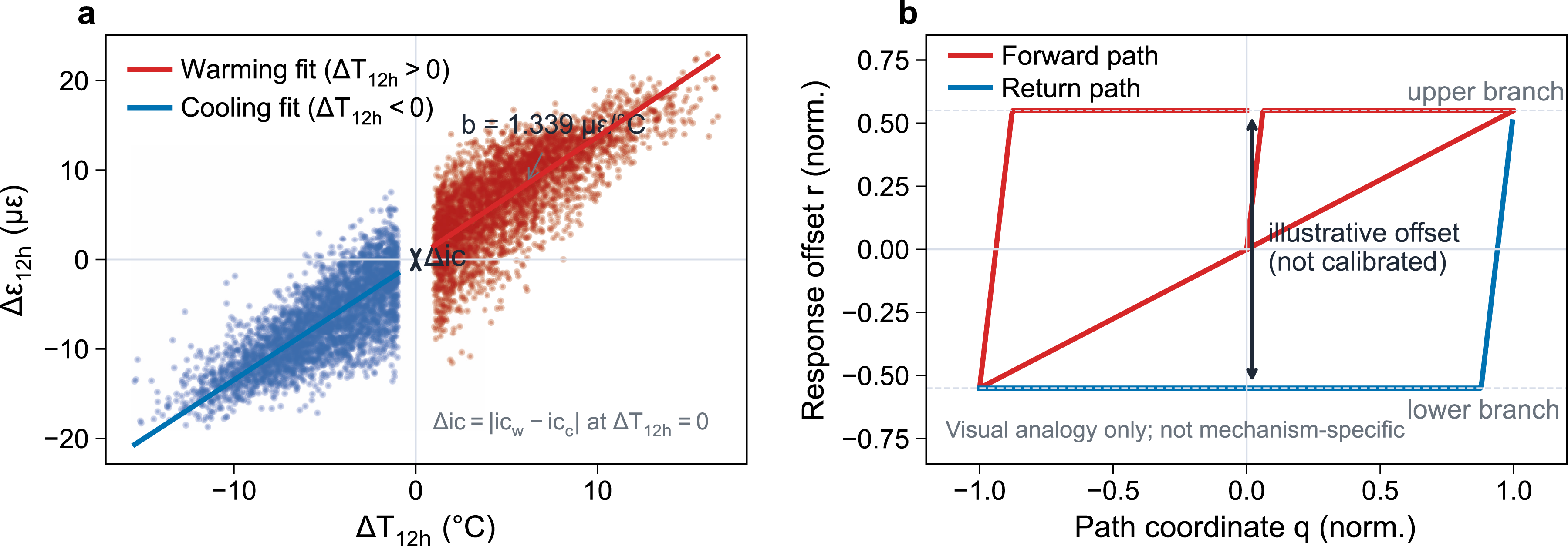

Evaluation metrics and temporal analysis

The branch regressions are evaluated with the coefficient of determination computed separately for the warming and cooling branches. These values are used only as fit-quality indicators; they do not replace the physical interpretation of the extracted parameters. Two temporal views are then constructed. The yearly analysis summarizes the inter-annual behavior of the main slope descriptor b and the auxiliary asymmetry descriptor Δic for each span. The monthly analysis pools same-month results across years so that seasonal repeatability and span-to-span differences can be compared directly.

For reproducibility, the implemented BSTRA protocol is summarized below. The same fixed protocol is used for the reported indicators; sensitivity checks are used to assess robustness, not to select a separate parameter set for each span.

(1) Use the external-temperature channel as the fixed excitation proxy for each span.

(2) Estimate the fixed lag δ* from hourly-increment cross-correlation.

(3) Build ΔT_12h(t) and Δɛ_12h(t) with the common 12-h window and the span-specific lag.

(4) Discard missing pairs and pairs with |ΔT_12h| < 1.0°C.

(5) Split the retained pairs into warming and cooling branches by the sign of ΔT_12h.

(6) Fit the two branch regressions, extract the main slope descriptor b, and retain Δic only as an auxiliary asymmetry descriptor.

(7) Aggregate the retained estimates by year and by calendar month for temporal comparison.

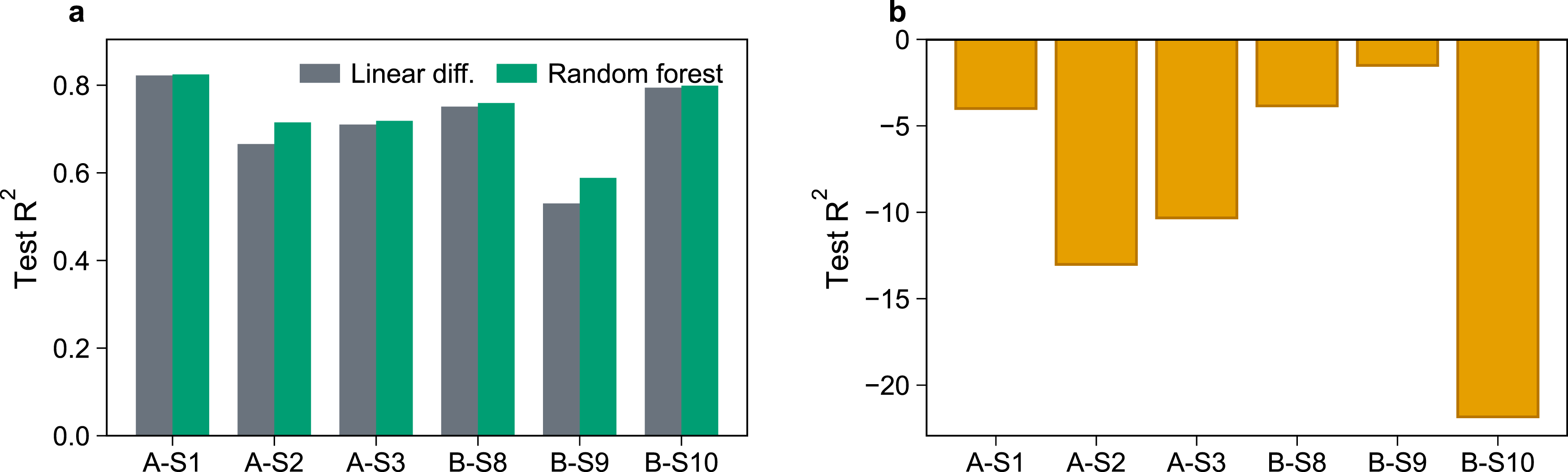
As supplementary benchmarks, five baseline or ablation methods are also considered: conventional raw-space linear regression, lag-corrected raw regression, lag-corrected differential regression without branch separation, raw-space branch splitting, and a light random-forest predictor in the lag-corrected differential space. The random-forest baseline uses the same sparse sensor configuration and simple temperature-increment, branch-sign, month, and concurrent-temperature features, with no further hyperparameter tuning. Its purpose is not to claim a state-of-the-art predictor, but to check whether an ordinary nonlinear regressor already extracts most of the predictive information available in the BSTRA input space (Kromanis and Kripakaran, 2017; Radicioni et al., 2025; Miranda et al., 2025; Zhou et al., 2024; Yue et al., 2022; Gong et al., 2024). For the predictive baseline, the hold-out year is 2021 for Bridge A and 2023 for Bridge B.

Because Δic is auxiliary, its bootstrap uncertainty and a normalized excitation-amplitude check are reported in the supplemental material and are not used as primary evidence in the main interpretation.

Results

Validation of lag correction and branch separation

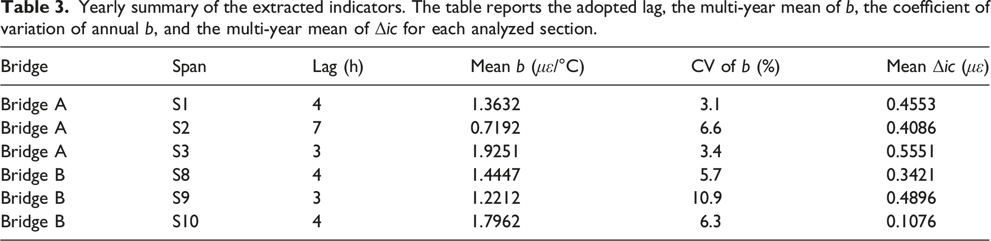
The selected lags are stable at the span level. The edge spans use lags of 3-4 h, whereas the Bridge A mid-span S2 requires a larger lag of 7 h. The yearly lag check shows no systematic drift within the retained analysis windows, which supports the use of fixed span-specific lag values in the subsequent calculations. The larger lag at S2 is consistent with a slower effective thermal response in the mid-span region than at the edge spans. One plausible reading is that the web-bottom strain at S2 reflects section-level heat diffusion and continuity-induced redistribution, in addition to the local external-temperature change.

To evaluate the practical effect of this alignment step without relying on selected examples, Figure 7 summarizes the monthly fit-quality gain for all six monitored sections using $Δ R^{2} = R_{corrected}^{2} - R_{uncorrected}^{2}$ . Positive values dominate across all sections, including Bridge A mid-span S2, which is otherwise the more difficult case. In this figure, the faint points are individual month–year ΔR² values from the retained records, lightly jittered along the calendar-month axis to reduce overplotting. The boxplots and the solid marker line summarize the same values as the within-month spread and monthly median. Lag correction improves branch-fit quality consistently across monitored sections, not only at a few isolated locations. The figure works here as a cross-section check of the lag-correction benefit. A seasonal tendency is also visible, with larger gains in several non-summer months, although the strength of that pattern differs among sections. This improvement supports the internal consistency of the workflow, but it does not by itself validate the mechanical interpretation of the extracted indicators.

Figure 7.

Monthly branch-fit improvement after lag correction. Faint points show individual month–year ΔR² values from the retained records and are lightly jittered along the month axis only to reduce overplotting. Boxplots summarize the within-month spread, and the solid marker line shows the monthly median.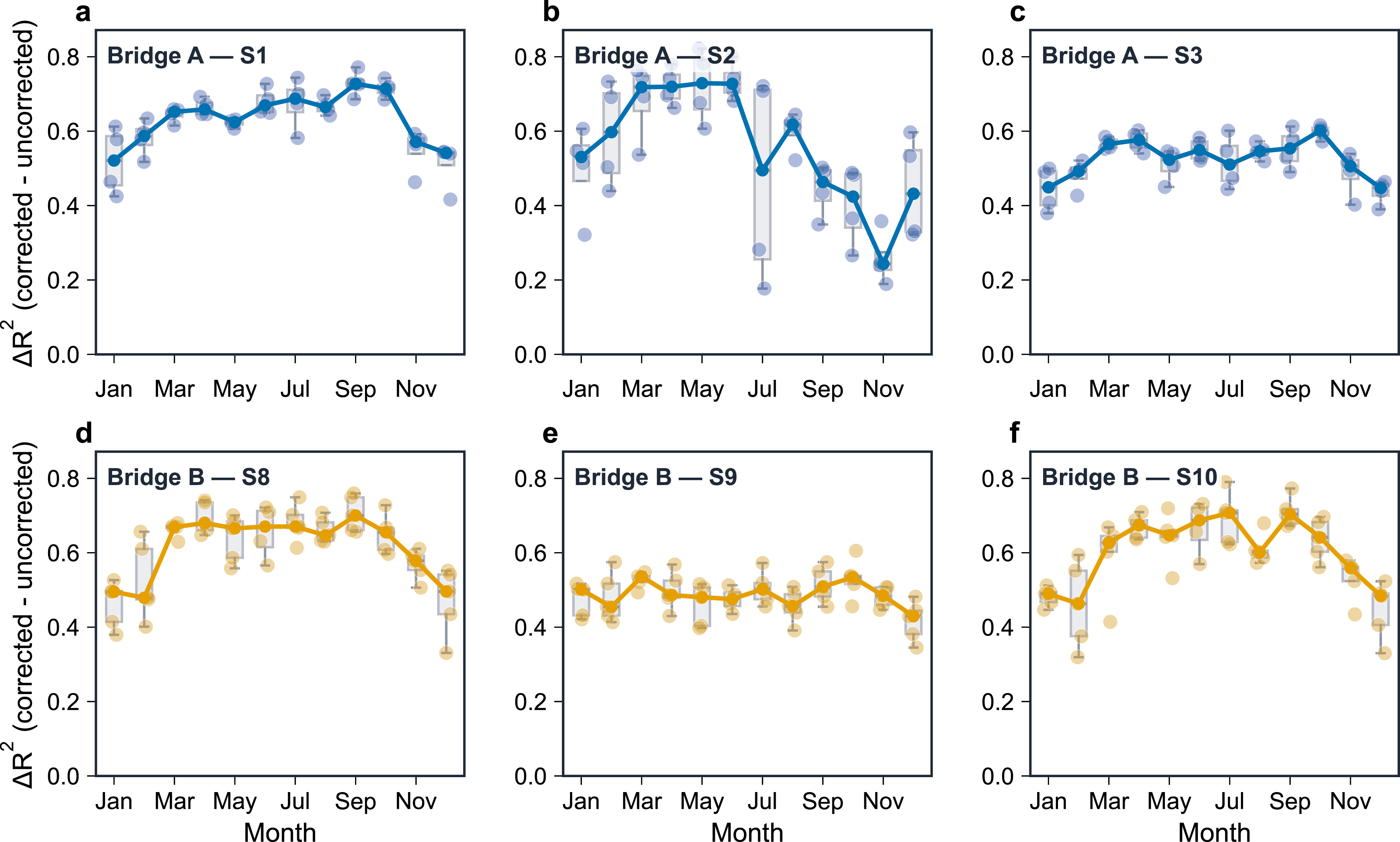

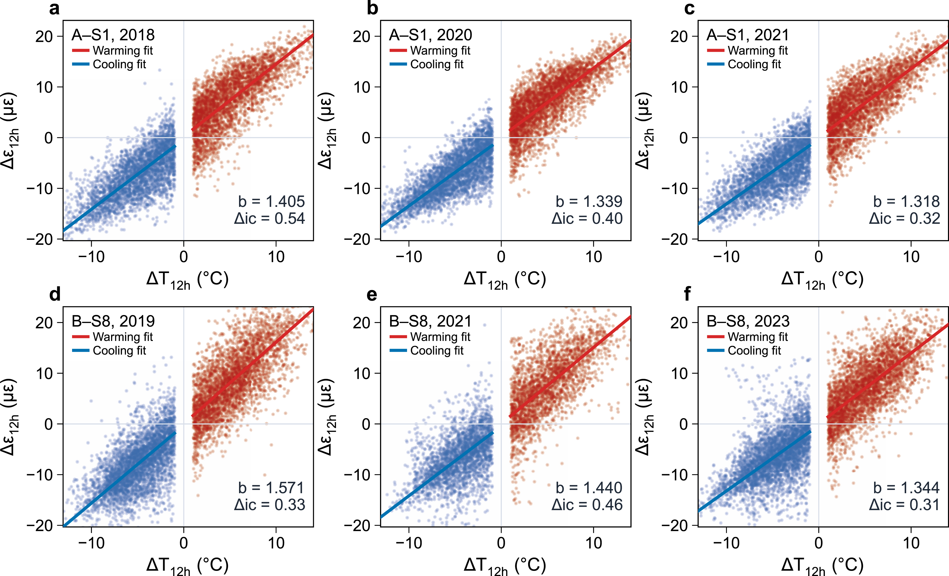
To address the visual effect of the preprocessing, Figure 8 first shows the raw-space branch plots before BSTRA is applied. Figure 9 then shows the corresponding results after lag correction and 12-h differencing. The two figures use the same six span-year cases and the same panel order, so each panel can be compared directly with its counterpart. The comparison is between analysis spaces, not between identical coordinate scales. In raw space, the point clouds remain broad and are affected by hysteresis and slow drift. In the BSTRA space, the same records form more compact warming and cooling branches, and the fitted branch slopes are more consistent across years. This comparison supports the use of the lag-corrected differential space for extracting the slope descriptor b. The intercept gap Δic remains comparatively small and more variable, so it is treated only as auxiliary path-asymmetry information.

Figure 8.

Raw-space temperature–strain branch plots before BSTRA preprocessing. The six panels show the same span-year cases and the same panel order as Figure 9: Bridge A–S1 in 2018, 2020, and 2021 in the top row, and Bridge B–S8 in 2019, 2021, and 2023 in the bottom row. Warming and cooling points are separated by the sign of the one-hour temperature increment. The records are quality-controlled but are not lag-corrected or 12-h differenced.

Figure 9.

Branch-separated fits after applying the BSTRA preprocessing to the same six span-year cases shown in Figure 8. The panel order is unchanged. The data are shown in the lag-corrected 12-h differential space, where warming and cooling branches are fitted separately to extract b and Δic.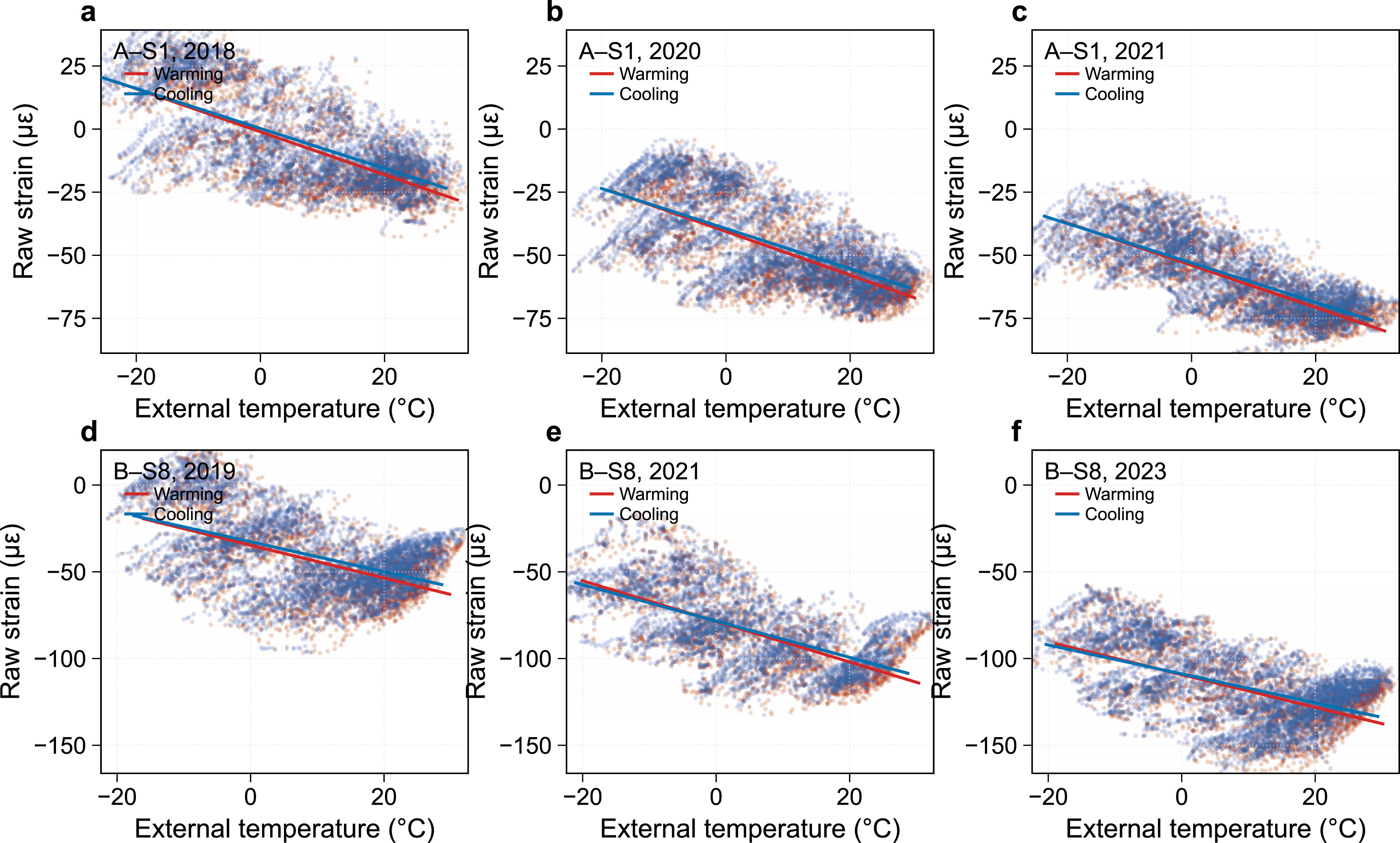

Comparison with baseline methods

Table 2 summarizes the baseline and ablation comparison. In the raw temperature–strain space, a single linear regression performs poorly for out-of-year prediction, with a mean test-set R² of −9.09 across the six monitored sections. This negative value is kept because it is the standard out-of-sample R² relative to the hold-out-year mean. It signals that raw-space regression collapses under year-to-year drift and hysteresis, not that the regression itself failed numerically. Moving to the lag-corrected differential space improves matters substantially: the simple no-branch differential linear model reaches a mean test-set R² of 0.712, and the random-forest baseline increases that value only modestly to 0.734.

Table 2.

Comparison of BSTRA with representative baseline and ablation methods. Predictive models are evaluated by hold-out year testing (Bridge A: 2021; Bridge B: 2023). For no-branch ablations, the fit-quality and CV columns refer to the single fitted slope in the corresponding analysis space.

Method	Analysis space	Mean test R²	Mean fit R²	Mean annual CV of b (%)
Raw linear regression	Raw T-ɛ	−9.09	—	—
Lag-corrected raw regression	Lag-corrected raw T-ɛ	—	0.176	79.2
Differential linear model	Lag-corrected ΔT-Δɛ	0.712	—	—
12-h differential regression	ΔT-Δɛ, no lag correction, no branch split	—	0.153	9.5
Lag-corrected differential regression	Lag-corrected ΔT-Δɛ, no branch split	—	0.736	6.0
Random-forest baseline	Lag-corrected ΔT-Δɛ	0.734	—	—
Raw branch splitting	Raw branch regressions	—	0.182	105.8
BSTRA	Lag-corrected differential branch regressions	—	0.738	6.0

Method	Mean monthly b amplitude (%)	Interpretation
Lag-corrected raw regression	113.7	Lag alone does not remove slow-drift instability
12-h differential regression	96.8	Differencing alone reduces drift but leaves poor thermal-response alignment
Lag-corrected differential regression	35.6	Stable central slope after lag correction and differencing
Raw branch splitting	135.9	Unstable branch indicator in raw space
BSTRA	35.6	Stable slope plus auxiliary branch check

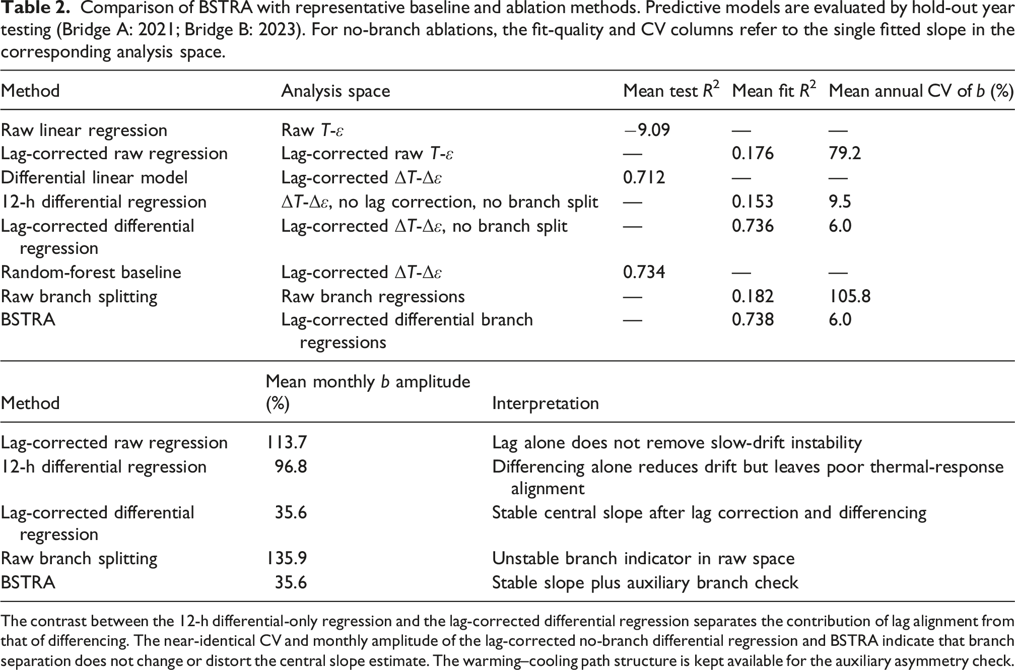
The contrast between the 12-h differential-only regression and the lag-corrected differential regression separates the contribution of lag alignment from that of differencing. The near-identical CV and monthly amplitude of the lag-corrected no-branch differential regression and BSTRA indicate that branch separation does not change or distort the central slope estimate. The warming–cooling path structure is kept available for the auxiliary asymmetry check.

The ablation isolates the contributions of differencing, lag correction, and branch separation. A 12-h differential regression without lag correction already brings the annual slope CV down to 9.5%, but the mean fit quality stays low (R² = 0.153) and the monthly slope amplitude remains large (96.8%). Adding span-specific lag correction to the same 12-h differential regression raises the mean fit quality to 0.736, drops the mean annual CV to 6.0%, and reduces the monthly amplitude to 35.6%. Full BSTRA gives essentially the same stability for b (R² = 0.738, annual CV 6.0%) while preserving the warming–cooling branch structure for the auxiliary asymmetry check. The pattern attributes each role separately. Differencing suppresses slow drift. Lag correction provides the main alignment gain. Branch separation adds little to the stability of b itself; it is kept to document whether residual warming–cooling asymmetry remains after differencing. Direct raw-space branch splitting performs worst among the indicator methods—mean branch-fit quality 0.182, annual b CV 105.8%, monthly b amplitude 135.9%.

Figure 10 visualizes the section-level stability contrast between BSTRA and raw-space branch splitting. Across all six monitored sections, BSTRA keeps the annual coefficient of variation of b within a much narrower range while also delivering higher branch-fit quality. The no-branch ablation in Table 2 indicates that this stabilization is mainly caused by the lag-corrected differential transformation. Figure 11 shows the prediction-side comparison. In the differential space, the random-forest baseline improves the test-set R² only modestly over the simple linear model, whereas direct raw-space regression remains unsuitable for this problem.

Figure 10.

Span-level stability comparison between BSTRA and raw-space branch splitting.

Figure 11.

Prediction-baseline comparison for the hold-out year tests.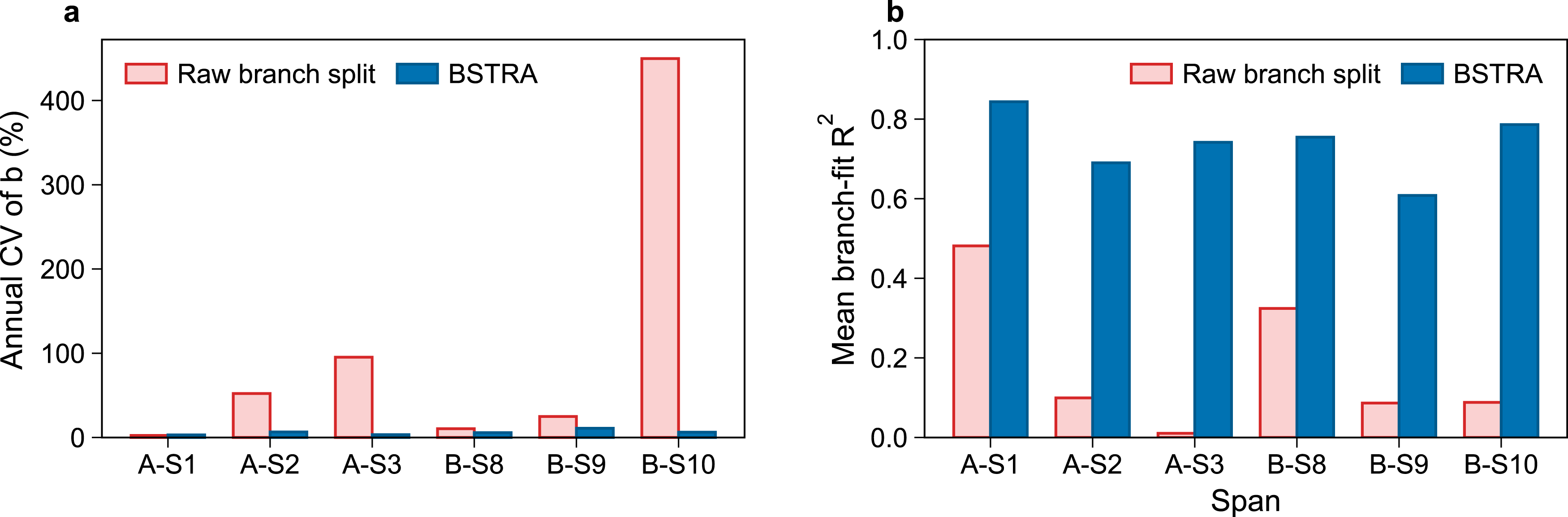

Annual stability of b and auxiliary branch asymmetry

The yearly results in Table 3 and Figure 12 show that b stays comparatively stable in most spans. For the edge spans, the coefficient of variation of annual b is 3.1% in Bridge A S1, 3.4% in Bridge A S3, 5.7% in Bridge B S8, and 6.3% in Bridge B S10. Bridge A mid-span S2 remains in a similar range at 6.6%, while Bridge B mid-span S9 reaches 10.9%. In these two bridges, the edge-span thermal bending response is fairly repeatable from year to year, while mid-span behavior is less uniform.

Table 3.

Yearly summary of the extracted indicators. The table reports the adopted lag, the multi-year mean of b, the coefficient of variation of annual b, and the multi-year mean of Δic for each analyzed section.

Bridge	Span	Lag (h)	Mean b (μɛ/°C)	CV of b (%)	Mean Δic (μɛ)
Bridge A	S1	4	1.3632	3.1	0.4553
Bridge A	S2	7	0.7192	6.6	0.4086
Bridge A	S3	3	1.9251	3.4	0.5551
Bridge B	S8	4	1.4447	5.7	0.3421
Bridge B	S9	3	1.2212	10.9	0.4896
Bridge B	S10	4	1.7962	6.3	0.1076

Figure 12.

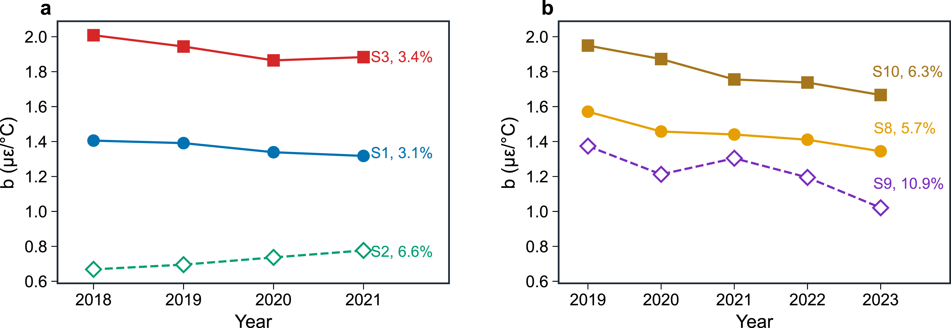
Yearly variation of b for the analyzed sections.

Δic remains small, with annual means from 0.11 to 0.56 μɛ across the analyzed sections. These values are reported only to document residual branch asymmetry after differential preprocessing; the supplemental bootstrap check shows that low-amplitude cases can be uncertain, so Δic is not used as a second structural state variable.

Monthly and seasonal evolution

The monthly syntheses in Figures 13 and 14 show a clear seasonal structure in b. In each bridge-specific figure, the thick mean curves carry the main trend, and the monthly error bars indicate the inter-annual standard deviation for the same calendar month. The blue winter shading denotes the conventional meteorological winter months December–February, and the orange summer shading denotes June–August. The bands are calendar-month guides used for visual interpretation, not temperature-threshold filters; the actual regression samples are selected by the fixed weak-excitation criterion |ΔT_12h|≥ 1.0°C described above. The seasonal amplitude of a span is defined throughout this paper as the maximum monthly mean of b minus the minimum monthly mean, divided by the absolute mean of the monthly means. The four edge spans share a common shape. Monthly b is higher in the cold season and lower in the warm season, with seasonal amplitudes from roughly 13% to 44% depending on the span. The monthly means are few and seasonally dependent, so we do not rely on a formal cold-versus-warm significance test. The interpretation rests on three things: the effect size, the repeated seasonal shape, and the contrast between spans. The span-to-span difference is visible in two ways at once—in the amplitude of the seasonal cycle, and in how distinctly the seasonal separation shows up in the available monthly samples.

Figure 13.

Monthly seasonality summary for Bridge A. Blue shading marks meteorological winter (December–February, shown as January–February and December on the January–December axis), and orange shading marks meteorological summer (June–August). The right blue segment covers December only and does not extend into November. The shading is a visual seasonal guide, not a temperature-threshold selection rule.

Figure 14.

Monthly seasonality summary for Bridge B. Blue shading marks meteorological winter (December–February, shown as January–February and December on the January–December axis), and orange shading marks meteorological summer (June–August). The right blue segment covers December only and does not extend into November. The shading is a visual seasonal guide, not a temperature-threshold selection rule.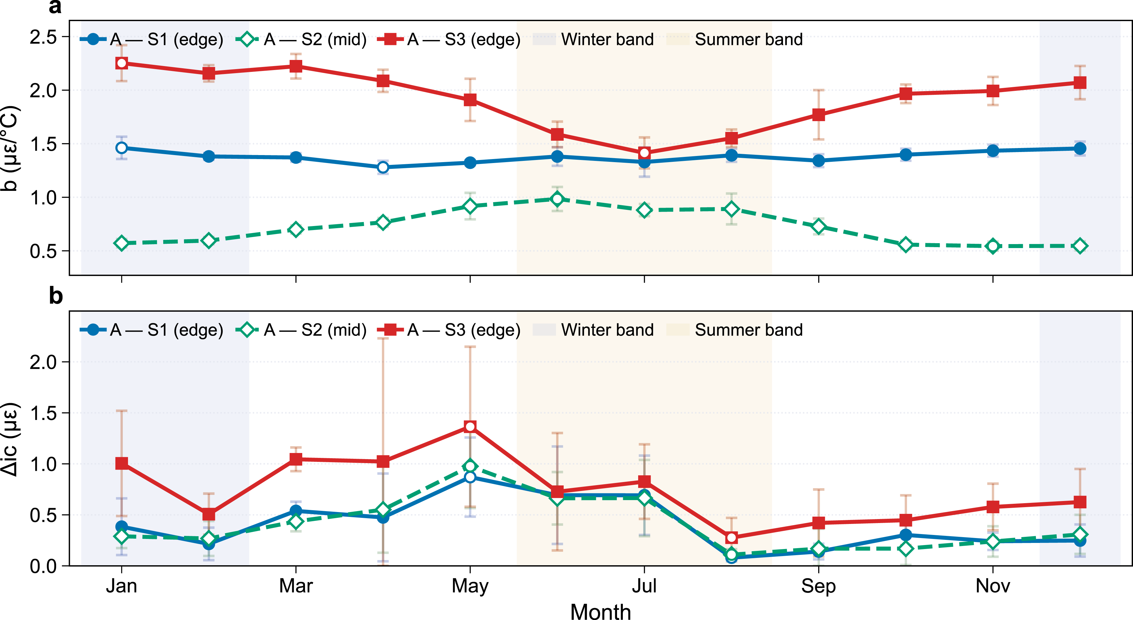

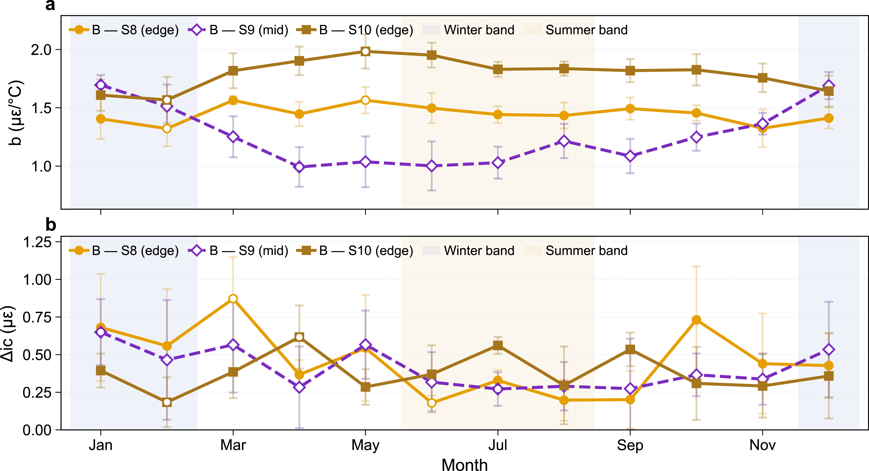
The mid-span behavior is different. Bridge A S2 reverses the seasonal direction: b is lower in winter and higher in late spring and summer, and the monthly amplitude reaches 60.9% under the same definition. This is well above any edge-span amplitude in either bridge. Bridge B S9 also breaks the edge-span pattern, but along a different axis. Its peak still occurs in winter, but the monthly amplitude reaches 55.8%, and its year-to-year variability of b is substantially higher than at the neighboring edge spans (annual CV 10.9%, vs 5.7% at S8 and 6.3% at S10). The two mid-spans break the edge-span signature in different forms. Section region is part of what shapes the seasonal pattern, even though the present dataset cannot identify the responsible bridge-specific factors. Mid-span sections should not be pooled with edge spans when seasonal baselines are built.

The lower rows of Figures 13 and 14 show the auxiliary Δic series; these patterns are less uniform than b and are not used as primary monitoring evidence.

Cross-span and cross-bridge comparison

The four edge spans behave consistently in two respects: their annual b values stay comparatively stable, and their monthly b values follow a repeatable seasonal cycle. The amplitude of that cycle differs by span. The direction does not—the cold-season increase appears in Bridge A S1, Bridge A S3, Bridge B S8, and Bridge B S10.

The two mid-span sections do not follow the same pattern. Bridge A S2 shows a seasonal direction opposite to the edge spans. Bridge B S9 keeps the edge-span direction but at a larger amplitude and with higher year-to-year variability than its neighboring edge spans. The size and form of these departures argue for treating edge-span and mid-span baselines separately, instead of pooling them.

Cross-bridge comparison in the rest of the paper therefore focuses on b. Δic is kept as auxiliary branch-asymmetry context, not as a primary cross-span descriptor.

Discussion

Interpretation of b as a section-level thermal-response slope

For the four edge spans, the seasonal behavior of b lines up with what one would expect from several mechanisms acting together. Cold-season b is higher than warm-season b in both bridges, and the year-to-year variation stays modest—annual CV between 3.1% and 6.3%. Several mechanisms can produce this direction. Concrete stiffness and thermal stresses change with temperature (Wu et al., 2022; Léger and Leclerc, 2002). Asphalt surfacing stiffens at low temperatures Judycki (2014). Through-section thermal gradients also vary seasonally and contribute to the measured slope. Because b absorbs all of these into a single fitted number, we read it as a section-level response quantity at the sensor location, not as a calibrated value of any one mechanical parameter.

The archived drawings provide the support context used in this discussion. For Bridge A, they tie the monitored S1–S3 unit to the A0–P1–P2–P3 support group, with the fixed-bearing set at Pier 2. For Bridge B, they tie the monitored unit to the left-line P7–P10 support group, with the fixed-bearing set at Pier 8. These archive checks are used only to clarify the monitored three-span boundary context relevant to the discussion below; they are not treated as a full bearing-condition diagnosis or as direct bearing-force measurements.

The mid-span results show that this reading does not carry over uniformly to all structural regions of the same continuous girder. At Bridge A S2 the seasonal direction reverses; at Bridge B S9 the direction is preserved but the amplitude is much larger. Both observations indicate that the monitored mid-span web-bottom strain is shaped by conditions specific to the mid-span region—section continuity with adjacent spans, boundary and support behavior, and the local thermal-gradient field (Léger and Leclerc, 2002; Xia et al., 2013; Hedegaard et al., 2017; Roeder and Stanton, 1990; Yakut and Yura, 2002). In a continuous girder, thermal expansion and contraction are not converted into strain by the section alone. They are filtered through the longitudinal restraint system. Fixed bearings restrain translation and can convert uniform thermal expansion into axial force, whereas movable bearings release part of that action. The resulting support restraint can change the balance between axial strain and thermally induced bending strain at the web-bottom gauge. Since b is fitted as the strain increment per unit temperature increment, seasonal changes in this axial–bending partition appear directly as seasonal changes in b: a more restraint-dominated response changes the axial component of the gauge strain, whereas greater release or a different thermal-gradient field lets the curvature component contribute more strongly. When these components have opposite signs at a mid-span web-bottom gauge, the net seasonal direction of b can differ from the edge-span direction. The archived support layouts therefore provide a reasonable boundary-condition context for the observed edge-span versus mid-span differences. The reversal observed at Bridge A S2 is interpreted in this bounded sense: it is evidence that the mid-span thermal-response signature differs from the edge-span signature, not proof of one unique bearing mechanism. Among the available archive information, the fixed-versus-movable bearing layout is the most direct structural boundary context for this interpretation. The data are sufficient to support the edge–mid-span distinction itself. They are not sufficient to partition the responsible contributions among material stiffening, gradient effects, moment redistribution, support and bearing behavior, environmental loading, and sensor-side factors. Resolving that partition would need bridge-specific thermo-mechanical modeling supported by richer field measurements.

Thermal-response signatures as a section-region monitoring descriptor

The pattern in the results is not just variability between spans. The four edge spans of the two bridges share the same cold-season-high seasonal direction. The two mid-spans break that direction in different ways. The contrast holds under the perturbations we tested. Read together, these point to b carrying a section-region signature, not just a span-specific number. Three points support reading b this way when seasonal baselines are built:

(1) Cross-bridge consistency. All four edge spans show the cold-season-high signature. This is not only a statistical repeat; it is consistent with the expectation that edge spans with similar end-restraint context have a more similar axial–bending partition at the web-bottom gauge. The two bridges differ in three respects: their analysis windows do not overlap (2018–2021 vs 2019–2023), their annual thermal ranges differ by 7°C (67°C vs 60°C), and their site conditions differ (Bridge B crosses an active railway corridor). A coincidence reading would have to hold across all three.

(2) Mid-span departure on both bridges. Each bridge contributes exactly one mid-span to the analysis, and both mid-spans break the edge-span signature. Mechanically, this is plausible because mid-span web-bottom strain is more strongly affected by continuity with adjacent spans, moment redistribution, and the local thermal-curvature field than a simple edge-span baseline would imply. The direction of the break is not the same: S2 reverses, S9 retains the cold-season-high direction but amplifies it. The amplitude, however, is consistently large—above 55% at both mid-spans, exceeding every edge-span amplitude in either bridge.

(3) Robustness to protocol perturbations. Three sensitivity checks were run on the protocol settings. Varying the temperature threshold between 0.5 and 1.5°C shifts the mean annual b by less than 0.2%. Varying the differencing window between τ = 6 and τ = 18 h keeps both signature amplitude and direction within about 10% of the τ = 12 h baseline. Perturbing the calibrated lag by ± 1 h leaves the annual CV of b within the 2.6%–11.6% band, comparable to the 3.1%–10.9% range at the calibrated lag itself. The signatures do not depend on a particular tuning choice.

This has direct consequences for monitoring practice. If a single regression coefficient is fitted across all spans of a continuous girder, or a uniform thermal compensation is applied to all of them, the edge–mid-span distinction documented here is averaged out. The same applies to anomaly checks based on one global seasonal baseline: such a baseline tends to be too tight at edge spans, where the signature is small and stable, and too loose at mid-spans, where the signature is larger and bridge-specific. Span-specific reference bands of b, organized by section region, are therefore a practical choice in this setting for separating structural departures from seasonal mismatch. They are also low-cost to build. BSTRA uses the sparse monitoring channels already in place and runs on fixed analysis settings once the lag is calibrated.

The signature reading also places BSTRA within the broader literature on bridge monitoring data. Cointegration and statistical detrending (Peeters and De Roeck, 2001; Cross et al., 2011; Kromanis and Kripakaran, 2017; Radicioni et al., 2025) and data-driven temperature-effect models (Yue et al., 2022; Zhou et al., 2024; Gong et al., 2024; Miranda et al., 2025) both treat seasonal temperature variation as a confounder—something to remove before downstream analysis. Our results suggest a complementary reading: the seasonal pattern itself can carry section-region information about the structure, so removing it may discard useful signal, not only nuisance. BSTRA does not replace these approaches; it works at a different level. Cointegration and detrending work on residuals, while BSTRA works on slopes. The two views can be combined when both residual anomaly detection and seasonal thermal-response tracking are needed.

Auxiliary checks and predictive baselines

Δic is retained only to record residual branch asymmetry after lag correction and differencing. In the present data it is small, sampling-sensitive, and not calibrated to a unique mechanical parameter, so it is not used as a standalone damage indicator or as a primary structural-response descriptor. The supplemental bootstrap and normalized-excitation checks document this limitation without changing the main interpretation, which rests on the stability and seasonality of b.

Two additional checks support the practical setting of the analysis. Girder-end longitudinal displacement remains strongly correlated with external temperature in both bridges, with absolute correlation coefficients of about 0.94–0.95, supporting the use of external temperature as a practical excitation proxy. The random-forest baseline provides only a small average improvement over the differential linear model in hold-out prediction and does not produce a stable span-comparable descriptor with the same interpretive content as b.

Implications for bridge monitoring

Where does BSTRA fit in monitoring practice? Not as a replacement for inspection, model-based assessment, or direct diagnosis—those remain the primary tools for engineering decisions. BSTRA fills a narrower role. It produces a slope descriptor that can be tracked month by month and year by year, using the sparse temperature and strain channels already available on many in-service continuous box-girder bridges.

The most direct application is to build monthly reference bands of b for each span, organized by section region (edge vs mid-span at minimum), with bootstrap confidence intervals from the retained valid years. New records are then compared against the band that matches the span, instead of against a single global threshold. A departure outside the band is a flag, not a verdict. It still has to be read together with inspection records, structural analysis, and any other available field evidence before engineering action is decided. The benefit of using region-specific bands is that the flag carries context. The same numerical departure means different things at different sections: at an edge span it stands out against a small, stable cold-season-high signature; at a mid-span it stands out against the larger, region-specific signature documented here.

The sensor demand of this workflow is the demand of the monitoring system that already exists on the analyzed bridges: one external-temperature, one internal-temperature, and one strain channel per span. No new instrumentation is implied. The broader methodological implication is that lag correction and differential branch separation, applied as a fixed protocol, can convert multi-year records that are routinely archived but rarely interpreted into a repeatable cross-span comparison tool, while the physical interpretation of the resulting indicators remains application-specific and grounded in the structural type and section region of the monitored locations.

Limitations

Four limitations affect the interpretation. First, the dataset contains no confirmed deterioration events, so the study cannot quantify how the extracted descriptors would behave under verified abnormal conditions. The signature view is descriptive in this respect: it shows that edge spans and mid-spans need different seasonal reference behavior in the present data, but it does not set thresholds for separating damage from normal seasonal variation. Second, the monitoring records provide sparse temperature and strain channels rather than a full thermal-field description. External air temperature is therefore used as a practical excitation proxy for cross-section comparison; it is not a complete thermal-boundary measurement. Third, Δic remains exploratory. It is not calibrated against independent mechanical measurements or against richer temperature-field observations, and the warming and cooling branches are often only weakly separated, which makes Δic more sensitive to regression noise and sampling variability than its notation may suggest. Fourth, the six-section design lets the protocol claim and the section-region claim be evaluated together, but the bridge sample is still small. The study should be read as two-bridge case evidence, not as a general law for all continuous box-girder bridges.

Further work should therefore test the descriptor and the signature view against confirmed abnormal cases, against richer thermo-mechanical measurements that can resolve the through-section gradient component, and against bridge-specific modeling that can better separate material, structural-region, and traffic effects. Extension to other continuous box-girder bridge types and to other cold-region climates would also help establish the boundaries of the edge-versus-mid-span signature reported here. These constraints do not invalidate the present observations, but they do bound the scope of generalization.

Conclusions

We started from a common monitoring situation: multi-year temperature and strain records are available, but the sensor layout is sparse. BSTRA uses those records without adding new measurements. It first aligns each monitored section by its calibrated thermal lag, then applies a 12-h difference and fits warming and cooling branches in the differential space. In the two bridge cases analyzed here, this fixed protocol makes the section-level slope b much more repeatable. Across six monitored sections, the mean annual coefficient of variation decreases from 105.8% in raw branch splitting to 6.0%, and the mean branch-fit R² increases from 0.182 to 0.738. The ablation results are also clear. Differencing alone improves stability but leaves poor fit quality. Adding lag correction provides the main gain in both stability and fit. Branch separation contributes little to b itself; it is kept only for the auxiliary warming–cooling asymmetry check.

With b stabilized, the span-region pattern becomes visible. The four edge spans have the same seasonal direction: b is higher in the cold season and lower in the warm season. Their monthly amplitudes range from 13% to 44%, and their annual coefficients of variation remain between 3.1% and 6.3%. The two mid-spans behave differently. Bridge A S2 reverses the seasonal direction and reaches a 60.9% monthly amplitude. Bridge B S9 keeps the cold-season-high direction, but its amplitude reaches 55.8% and its annual variability is higher (10.9%). The pattern remains under the tested window, threshold, and lag perturbations. A single seasonal baseline would hide part of this structure. For monitoring practice, a more defensible choice in these cases is to build monthly b reference bands by span region and then screen new departures against the appropriate band.

The main value of the work is both methodological and empirical. We show that sparse records already stored in bridge management systems can be processed into a span-comparable thermal-response descriptor when lag, differencing window, and branch fitting are handled consistently. We also document, in two bridge cases, a seasonal difference between edge-span and mid-span sections that should be considered when monitoring baselines are built. The evidence is still case-based. Future work should test the descriptor on bridges with confirmed abnormal events, richer thermal-field measurements, and other continuous-girder forms and climates.

Supplemental material

Supplemental Material - Edge- and mid-span thermal-response signatures in continuous box-girder bridges

Supplemental Material for Edge- and mid-span thermal-response signatures in continuous box-girder bridges by Wande Li, Longsheng Bao, Jinliang Liu and Fengqi Lu in Advances in Structural Engineering.

Footnotes

Acknowledgements

The authors thank the bridge management agencies for providing monitoring data support.

ORCID iD

Wande Li

Ethical considerations

Ethical approval was not required for this study because it used structural monitoring data from operating bridges and did not involve human participants, human data, or human tissue.

Author contributions

Wande Li: Conceptualization, methodology, software, formal analysis, visualization, writing–original draft. Longsheng Bao: Supervision, resources, data curation, writing–review and editing. Jinliang Liu: Methodology, validation, writing–review and editing. Fengqi Lu: Resources, investigation, writing–review and editing.

Funding

The authors disclosed receipt of the following financial support for the research, authorship, and/or publication of this article: This work was supported by the Liaoning Provincial Transportation Investment Group Co., Ltd. (Liaoning Communications Investment Group) under Science and Technology Project Grant No. 202303. The funder had no role in the study design, data analysis and interpretation, manuscript preparation, or decision to submit the article for publication.

Declaration of conflicting interests

The authors declared no potential conflicts of interest with respect to the research, authorship, and/or publication of this article.

Data Availability Statement

The monitoring data used in this study involve sensitive safety information from operating bridges and are therefore not publicly available. Reasonable requests may be considered by the corresponding author.*

Code availability

The processing workflow is fully specified by the equations, thresholds, and stepwise protocol reported in this paper. The project scripts were developed for the monitored bridge records and are not publicly released because the underlying data involve operating infrastructure. Representative pseudocode or implementation details may be provided by the corresponding author upon reasonable request.

Declaration of generative AI and AI-assisted technologies in the manuscript preparation process

During manuscript preparation, the authors used AI-assisted tools for limited language polishing, drafting refinement, and coding support. All technical decisions, analyses, result checks, and the final wording of the manuscript were reviewed and approved by the authors, who take full responsibility for the content.

Supplemental material

Supplemental material for this article is available online.

References

Abdel-Jaber

Glisic

(2019) Monitoring of long-term prestress losses in prestressed concrete structures using fiber optic sensors. Structural Health Monitoring 18(1): 254–269. https://doi.org/10.1177/1475921717751870

Brownjohn

JMW

(2007) Structural health monitoring of civil infrastructure. Philosophical Transactions of the Royal Society A: Mathematical, Physical and Engineering Sciences 365(1851): 589–622. https://doi.org/10.1098/rsta.2006.1925

Cao

Yim

Zhao

, et al. (2011) Temperature effects on cable stayed bridge using health monitoring system: a case study. Structural Health Monitoring 10(5): 523–537. https://doi.org/10.1177/1475921710388970

Cardini

DeWolf

(2009) Long-term structural health monitoring of a multi-girder steel composite bridge using strain data. Structural Health Monitoring 8(1): 47–58. https://doi.org/10.1177/1475921708094789

Cross

Worden

Chen

(2011) Cointegration: a novel approach for the removal of environmental trends in structural health monitoring data. Proceedings of the Royal Society A 467(2133): 2712–2732. https://doi.org/10.1098/rspa.2011.0023

Cury

Cremona

(2012) Assignment of structural behaviours in long-term monitoring: application to a strengthened railway bridge. Structural Health Monitoring 11(4): 422–441. https://doi.org/10.1177/1475921711434858

Deraemaeker

Reynders

De Roeck

, et al. (2008) Vibration-based structural health monitoring using output-only measurements under changing environment. Mechanical Systems and Signal Processing 22(1): 34–56. https://doi.org/10.1016/j.ymssp.2007.07.004

Enckell

Glisic

Myrvoll

, et al. (2011) Evaluation of a large-scale bridge strain, temperature and crack monitoring with distributed fibre optic sensors. Journal of Civil Structural Health Monitoring 1(1–2): 37–46. https://doi.org/10.1007/s13349-011-0004-x

Farrar

Worden

(2007) An introduction to structural health monitoring. Philosophical Transactions of the Royal Society A: Mathematical, Physical and Engineering Sciences 365(1851): 303–315. https://doi.org/10.1098/rsta.2006.1928

10.

Farreras-Alcover

Chryssanthopoulos

Andersen

(2015) Regression models for structural health monitoring of welded bridge joints based on temperature, traffic and strain measurements. Structural Health Monitoring 14(6): 648–662. https://doi.org/10.1177/1475921715609801

11.

Gong

Song

, et al. (2024) Deep learning based anomaly identification of temperature effects in bridge structural health monitoring data. Structures 69: 107478. https://doi.org/10.1016/j.istruc.2024.107478

12.

Hedegaard

French

CEW

Shield

(2017) Time-dependent monitoring and modeling of I-35W St. Anthony Falls Bridge. I: analysis of monitoring data. Journal of Bridge Engineering 22(7): 04017025. https://doi.org/10.1061/(ASCE)BE.1943-5592.0001053

13.

Said

Rohrmann

, et al. (2018) Continuous dynamic monitoring of a prestressed concrete bridge based on strain, inclination and crack measurements over a 14-year span. Structural Health Monitoring 17(5): 1073–1094. https://doi.org/10.1177/1475921717735505

14.

Yan

Xie

, et al. (2022) Statistical analysis of the vertical temperature gradient of the web plate of steel box girder bridges in cold regions. KSCE Journal of Civil Engineering 26(9): 3876–3887. https://doi.org/10.1007/s12205-022-0554-y

15.

Judycki

(2014) Influence of low-temperature physical hardening on stiffness and tensile strength of asphalt concrete and stone mastic asphalt. Construction and Building Materials 61: 191–199. https://doi.org/10.1016/j.conbuildmat.2014.03.011

16.

(2005) Technology developments in structural health monitoring of large-scale bridges. Engineering Structures 27(12): 1715–1725. https://doi.org/10.1016/j.engstruct.2005.02.021

17.

Kromanis

Kripakaran

(2017) Data-driven approaches for measurement interpretation: analysing integrated thermal and vehicular response in bridge structural health monitoring. Advanced Engineering Informatics 34: 46–59. https://doi.org/10.1016/j.aei.2017.09.002

18.

Nishio

(2015) Time-series analysis of GPS monitoring data from a long-span bridge considering the global deformation due to air temperature changes. Journal of Civil Structural Health Monitoring 5(4): 415–425. https://doi.org/10.1007/s13349-015-0124-9

19.

Léger

Leclerc

(2002) Evaluation of thermal deformation, stresses and cracking of concrete structures. Computers & Structures 80(16–17): 1363–1380. https://doi.org/10.1016/S0045-7949(02)00099-7

20.

Liu

DeWolf

Kim

(2009) Development of a baseline for structural health monitoring for a curved post-tensioned concrete box-girder bridge. Engineering Structures 31(12): 3107–3115. https://doi.org/10.1016/j.engstruct.2009.08.022

21.

Liu

Jiang

, et al. (2019) Long-term field test of temperature gradients on the composite girder of a long-span cable-stayed bridge. Advances in Structural Engineering 22(13): 2785–2798. https://doi.org/10.1177/1369433219851300

22.

Meixedo

Ribeiro

Santos

, et al. (2021) Progressive numerical model validation of a bowstring-arch railway bridge based on a structural health monitoring system. Journal of Civil Structural Health Monitoring. https://doi.org/10.1007/s13349-020-00461-w

23.

Miranda

Mata

Santos

, et al. (2025) Structural characterization of a suspension bridge by mapping the temperature effects on strain response based on neural network models. Journal of Civil Structural Health Monitoring 15(4): 1117–1137. https://doi.org/10.1007/s13349-024-00855-0

24.

Nepomuceno

Webb

Bennetts

, et al. (2022) Thermal monitoring of a concrete bridge in London, UK. Proceedings of the Institution of Civil Engineers – Bridge Engineering 175(1): 16–34. https://doi.org/10.1680/jbren.20.00012

25.

Hua

Fan

, et al. (2005) Correlating modal properties with temperature using long-term monitoring data and support vector machine technique. Engineering Structures 27(12): 1762–1773. https://doi.org/10.1016/j.engstruct.2005.02.020

26.

Peeters

De Roeck

(2001) One-year monitoring of the Z24-Bridge: environmental effects versus damage events. Earthquake Engineering & Structural Dynamics 30(2): 149–171. https://doi.org/10.1002/1096-9845(200102)30:2⟨149::AID-EQE1⟩3.0.CO;2-Z

27.

Radicioni

Giorgi

Benedetti

, et al. (2025) On the performance of data-driven dynamic models for temperature compensation on bridge monitoring data. Journal of Civil Structural Health Monitoring 15(6): 1957–1972. https://doi.org/10.1007/s13349-025-00920-2

28.

Ren

, et al. (2022) An anomaly pattern detection for bridge structural response considering time-varying temperature coefficients. Structures 46: 285–298. https://doi.org/10.1016/j.istruc.2022.10.020

29.

Roeder

Stanton

Feller

(1990) Low temperature performance of elastomeric bearings. Journal of Cold Regions Engineering 4(3): 113–132. https://doi.org/10.1061/(ASCE)0887-381X(1990)4:3(113)

30.

Sawicki

Bruhwiler

(2020) Long-term strain measurements of traffic and temperature effects on an rc bridge deck slab strengthened with an r-uhpfrc layer. Journal of Civil Structural Health Monitoring 10(2): 333–344. https://doi.org/10.1007/s13349-020-00387-3

31.

Sohn

(2007) Effects of environmental and operational variability on structural health monitoring. Philosophical Transactions of the Royal Society A: Mathematical, Physical and Engineering Sciences 365(1851): 539–560. https://doi.org/10.1098/rsta.2006.1935

32.

Sohn

Farrar

Hemez

, et al. (2003) A Review of Structural Health Monitoring Literature: 1996–2001. Technical Report LA-13976-MS. Los Alamos National Laboratory.

33.

Webb

Vardanega

Hoult

, et al. (2017) Analysis of fiber-optic strain-monitoring data from a prestressed concrete bridge. Journal of Bridge Engineering 22(5): 05017002. https://doi.org/10.1061/(ASCE)BE.1943-5592.0000996

34.

Zhang

(2022) Mechanical properties and damage constitutive model of concrete under low-temperature action. Construction and Building Materials 348: 128668. https://doi.org/10.1016/j.conbuildmat.2022.128668

35.

Xia

Chen

Weng

, et al. (2012) Temperature effect on vibration properties of civil structures: a literature review and case studies. Journal of Civil Structural Health Monitoring 2(1): 29–46. https://doi.org/10.1007/s13349-011-0015-7

36.

Xia

Chen

Zhou

, et al. (2013) Field monitoring and numerical analysis of Tsing Ma suspension bridge temperature behavior. Structural Control and Health Monitoring 20(4): 560–575. https://doi.org/10.1002/stc.515

37.

Xia

, et al. (2022) Temperature behaviors of an arch bridge through integration of field monitoring and unified numerical simulation. Advances in Structural Engineering 25(16): 3492–3509. https://doi.org/10.1177/13694332221130797

38.

Yakut

Yura

(2002) Parameters influencing performance of elastomeric bearings at low temperatures. Journal of Structural Engineering 128(8): 986–994. https://doi.org/10.1061/(ASCE)0733-9445(2002)128:8(986)

39.

Yan

Kerschen

De Boe

, et al. (2005) Structural damage diagnosis under varying environmental conditions—Part I: a linear analysis. Mechanical Systems and Signal Processing 19(4): 847–864. https://doi.org/10.1016/j.ymssp.2004.12.002

40.

Yang

Ding

Jiang

, et al. (2024) Time-lag effect of temperature-induced strain for concrete box girder bridges: field monitoring and fem study. Journal of Civil Structural Health Monitoring 14(2): 303–320. https://doi.org/10.1007/s13349-023-00725-1

41.

Yue

Ding

Zhao

, et al. (2022) Ultra-high precise Stack-LSTM-CNN model of temperature-induced deflection of a cable-stayed bridge for detecting bridge state driven by monitoring data. Structures 45: 110–125. https://doi.org/10.1016/j.istruc.2022.09.011

42.

Zhang

Liu

Deng

(2021) Temperature gradient modeling of a steel box-girder suspension bridge using Copulas probabilistic method and field monitoring. Advances in Structural Engineering 24(5): 947–961. https://doi.org/10.1177/1369433220971779

43.

Zhang

Wang

Chen

, et al. (2026) Climate change intensifies bridge temperature: evidence from 26 years of monitoring data. Advances in Structural Engineering 29(6): 1202–1213. https://doi.org/10.1177/13694332251377551

44.

Zhou

Sun

(2019) Insights into temperature effects on structural deformation of a cable-stayed bridge based on structural health monitoring. Structural Health Monitoring 18(3): 778–791. https://doi.org/10.1177/1475921718773954

45.

Zhou

Wang

Chen

(2024) Bridge temperature prediction method based on long short-term memory neural networks and shared meteorological data. Advances in Structural Engineering 27(8): 1349–1360. https://doi.org/10.1177/13694332241247918

46.

Zhou

Fan

Huang

, et al. (2025) Numerical calculation of bridge temperature considering all-weather conditions. Advances in Structural Engineering 28(15): 2925–2941. https://doi.org/10.1177/13694332251365967

47.

Zhu

Jesus

, et al. (2018) Thermal strain extraction methodologies for bridge structural condition assessment. Smart Materials and Structures 27(10): 105051. https://doi.org/10.1088/1361-665X/aad5fb

48.

Zhu

Ren

Wang

(2022) Structural health monitoring on Yangluo Yangtze River Bridge: implementation and demonstration. Advances in Structural Engineering 25(7): 1431–1448. https://doi.org/10.1177/13694332211069508

Supplementary Material

Please find the following supplemental material available below.

For Open Access articles published under a Creative Commons License, all supplemental material carries the same license as the article it is associated with.

For non-Open Access articles published, all supplemental material carries a non-exclusive license, and permission requests for re-use of supplemental material or any part of supplemental material shall be sent directly to the copyright owner as specified in the copyright notice associated with the article.

0.67 MB

0.00 MB