3-D Analytical Comparison of Axial Flux Machines With Layered and Segmented Halbach Magnets

Abstract

The three-dimensional (3-D) linear analytical comparison is made for axial flux machines (AFMs) with surface-mounted non-layered/layered and segmented Halbach magnets. Using a 3-D subdomain model method, the analytical equations in terms of the scalar potential for different subdomains are solved. In addition, the magnet parameters are optimized to enhance the performance of AFMs. It is well demonstrated that the optimized AFM with the radially layered unequal-height Halbach magnets exhibit better performance than that with the other magnet arrangements. Finally, the proposed 3-D linear analytical predictions are validated through a 3-D finite element analysis (FEA).

Keywords

3-D linear analytical comparison axial flux machine radially layered unequal-height Halbach electromagnetic performance

Introduction

Axial flux machines (AFMs) with permanent magnets have the advantages of relatively compact structure, low loss, high torque and power density. Thus they have a wide range of industrial and agricultural applications in the aerospace, national defense, transportation, and public life (Jin et al., 2015; Zhao et al., 2014).

AFMs can be classified by the topological structures, i.e., single-stator single-rotor, double-stator single-rotor, single-stator double-rotor, and multi-stator multi-rotor (Kahourzade et al., 2014; Nishanth et al., 2021). In order to reduce the unilateral magnetic force, the two-sided structure with the middle stator or rotor is the most widely used one (Gieras et al., 2008). Compared with the single-stator double-rotor AFM, the double-stator single-rotor AFM with flexibility design can use the magnetic field interaction generated by the two stators to increase the torque output, thus making it more advantageous in some specific applications with relatively high requirements (Ge et al., 2022).

In recent years, the academic research on the Halbach arrays for AFMs has aroused the widespread interest. Compared with the AFMs without Halbach arrays, AFMs with Halbach arrays offer many attractive advantages. The Halbach array is utilized for an AFM in (Habib et al., 2022), the magnet shape is optimized to obtain the higher performance. A high-speed Halbach-array rotor for ironless AFM is proposed and investigated in (Zhang et al., 2020). A kind of AFM with multi-segment Halbach array is proposed in (Okita & Harada, 2023). In order to increase the torque density, the combination of Halbach arrays is presented for the AFM with yokeless and segmented armature in (Lu et al., 2024). A novel magnet structure combining the block, trapezoidal and Halbach magnets is proposed and greatly increase the airgap flux density performance in (Yang et al., 2021). A novel radially layered magnet structure with tangentially magnetized magnets and radial Halbach array in parallel excitation is proposed in (Wang et al., 2021). The internal space is effectively utilized and the output performance is improved with the same main magnetic flux area.

Generally, a three-dimensional (3-D) finite element analysis (FEA) method can be used to solve the magnetic field in AFMs (Geng & Zhang, 2018; Sun et al., 2020). However, both the calculation and optimization of the 3-D FEA model often take a long time (Habib et al., 2022). Instead, the analytical method is preferred to predict the performances of the 3-D field AFMs. The analytical methods for the AFMs using a quasi-3D model or the dimensionality reduction processing not only have higher computational complexity and lead to great restrictions on the 3-D structure, but also have a relatively lower calculation accuracy (Sun et al., 2018; Zerioul et al., 2018). A 3-D analytical AFM model with the conventional magnet structure is proposed in (Jin et al., 2014), and the analytical formulas are presented to accurately gain the 3-D field parameters. For the 3-D analytical model of AFMs with Halbach arrays, the Fourier-Bessel equation is used to provide a more rigorous and widely applicable expression for the magnetic field, back electromotive force and torque (Jin et al., 2015; Okita & Harada, 2023).

In this paper, the AFM models with layered and segmented Halbach magnets are proposed and compared. All the compared AFMs are double-stator single-rotor arrangements. Using a 3-D analytical method, the electromagnetic performances of the slotted AFMs are analyzed, and the magnet parameter variables are optimized. With the equal remanence per unit volume for the magnets, the electromagnetic performance of the optimized model with radially layered and circumferentially segmented is obviously better than that of the other models. Finally, a 3-D FEA model is used to compare and verify the analytical prediction results.

AFM Physical Model

Figure 1(a)–(d) show four rotor structures of AFMs with different segmented Halbach magnet arrangements. Figure 1(a) shows the single-layer equal-height Halbach magnets with the same remanence for Machine I. Figure 1(b) shows the single-layer unequal-height Halbach magnets for Machine II. Figure 1(c) shows the proposed axially layered unequal-height Halbach magnets for Machine III. Figure 1(d) shows the proposed radially layered unequal-height Halbach magnets for Machine IV. It is noted that the three-segment magnets (i.e., each pole magnets) in Machines II, III and IV have different remanences and different magnetization angles. For a fair comparison, they share the same magnet remanence per unit volume.

Figure 1.

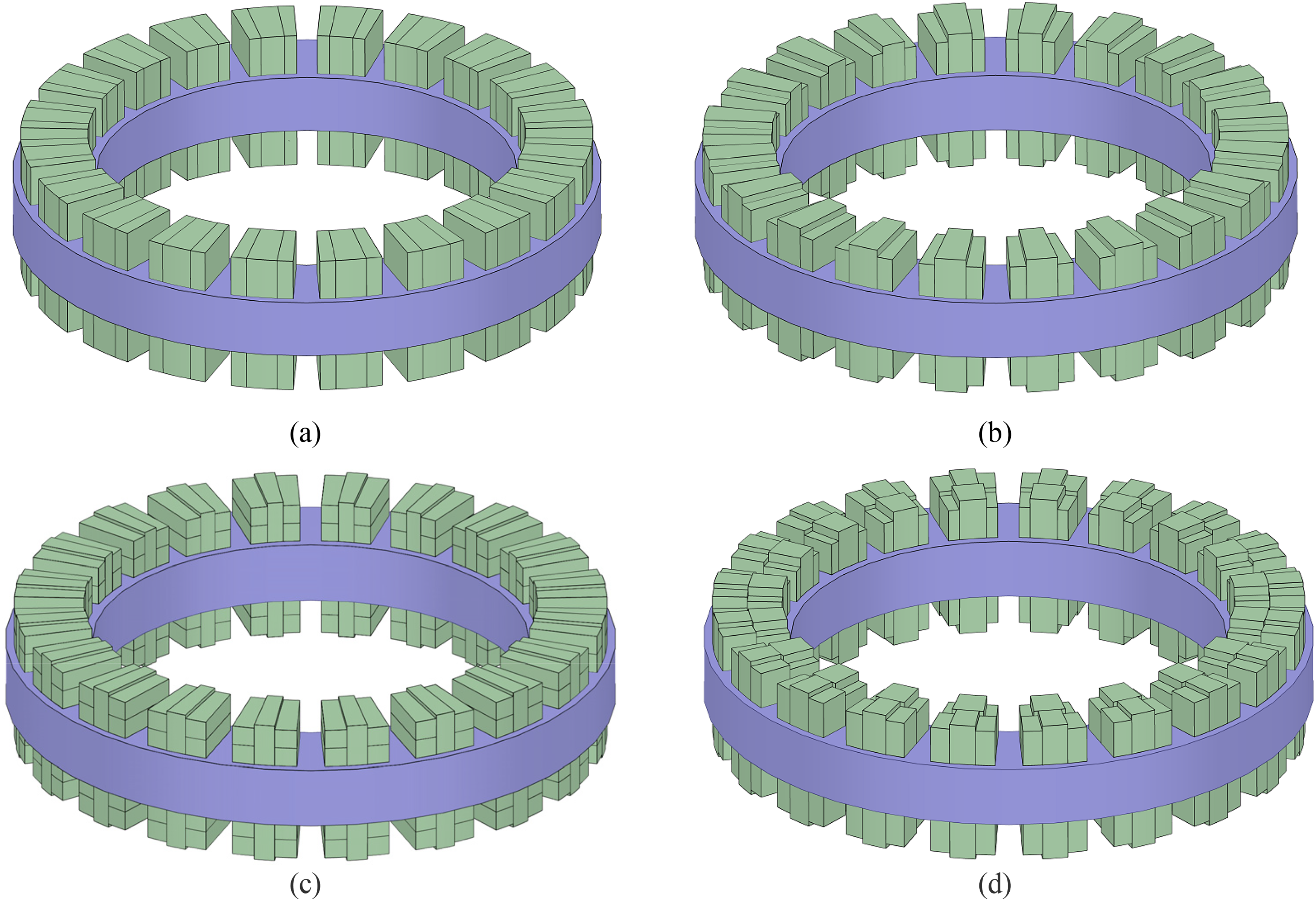
Four types of rotor PM arrangements. (a) Single-layer equal-height Halbach magnets for Machine I. (b) Single-layer unequal-height Halbach magnets for Machine II. (c) Proposed axially layered unequal-height Halbach magnets for Machine III. (d) Proposed radially layered unequal-height Halbach magnets for Machine IV.

Figure 2 shows the stator and rotor of a 3-D AFM with radially layered unequal-height Halbach magnets. The double-stator single-rotor arrangement is used.

Figure 2.

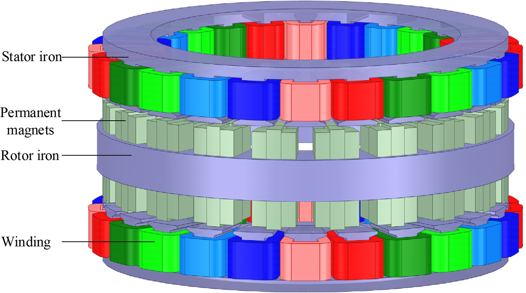
Stator and rotor of 3-D AFM with radially layered unequal-height Halbach magnets.

Figure 3 shows the rotor geometric parameters of the AFM from the top view. The inner and outer layer magnet arrays have the same arc angle. R_r₁ and R_r₂ are the inner/outer radii of the rotor iron. R_m₁, R_m₂ and R_m₃ are the inner radius of the inner layer magnet array, the outer radius of the inner layer magnet array (i.e., the inner radius of the outer layer magnet array) and the outer radius of the outer layer magnet array, respectively. β₁ is the pole pitch, β₂ is the arc angle of the three-segment Halbach magnet array, β₃ is the arc angle of the inner layer mid-magnet, and β₄ is the arc angle of the outer layer mid-magnet. α₁= β₂/β₁ is the polar arc ratio, α₂= β₃/β₂ and α₃= β₄/β₂ are the ratios of the inner and outer layer mid-magnet to the three-segment magnets, respectively.

Figure 3.

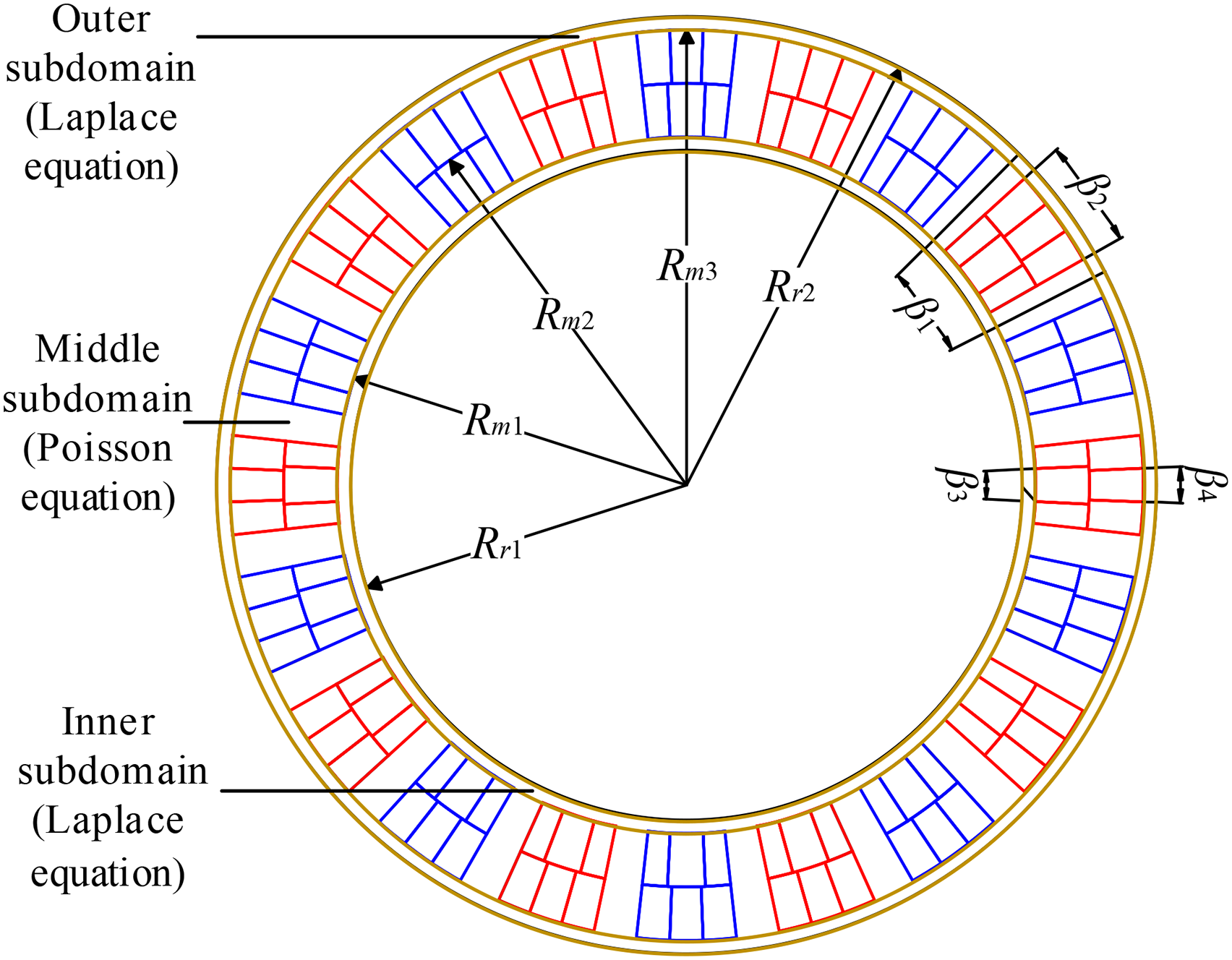
Rotor geometric parameters from the top view.

Figure 4 shows the parameters of outer and inner layers of the proposed radially layered model. The remanences of the mid-magnet and side-magnet are unequal. h₁ is the axial thickness of the mid-magnet, h₂ is the axial thickness of the rotor iron, h₃ and h₄ are the axial lengths of the outer and inner layer magnet, respectively. g₁ is the airgap length between the stator and the mid-magnets, g₂ and g₃ are the airgap lengths between the stator and the outer/inner layer side-magnets, respectively. θ₁ and θ₂ are two magnetization angles of the outer/inner layer side-magnets, respectively.

Figure 4.

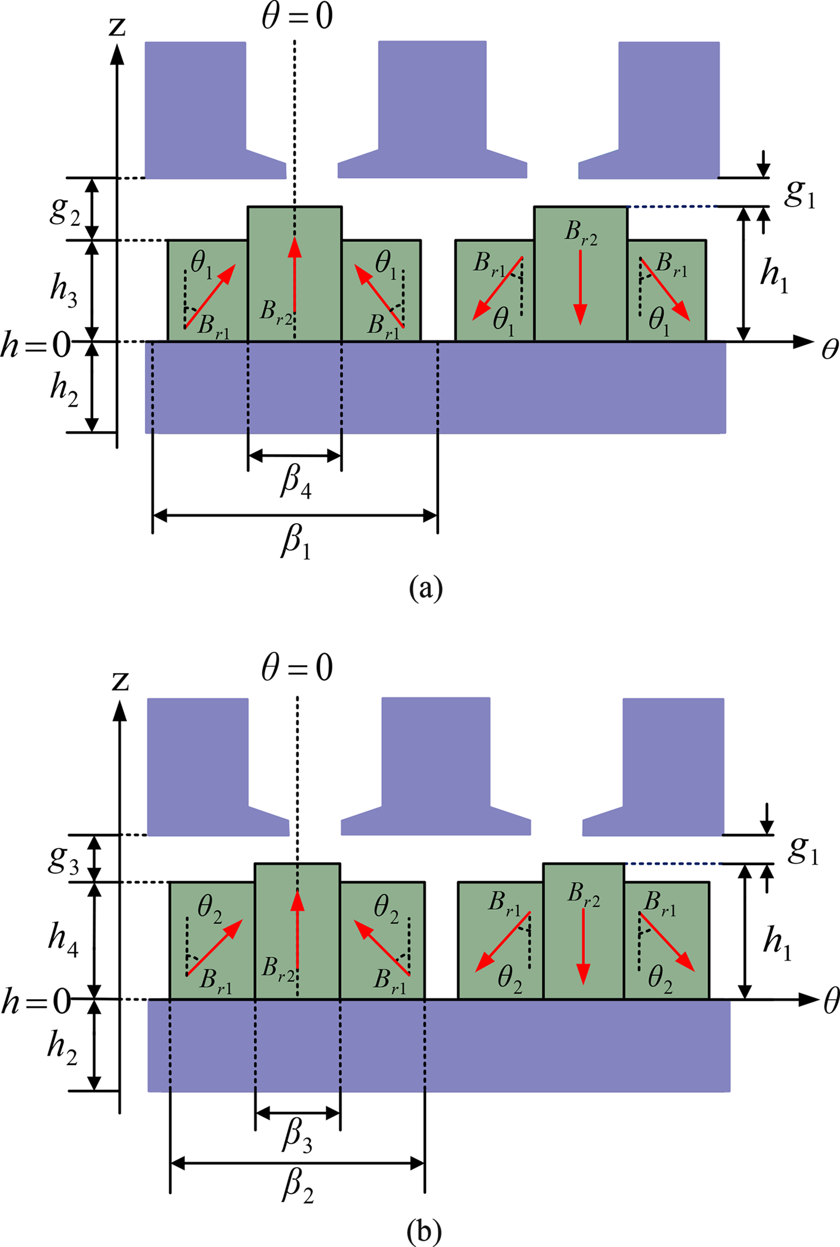
Parameters of outer and inner layers. (a) Outer layer. (b) Inner layer.

General Solution Equations for Subdomains

The initial spatial positions of analytical calculation are defined as θ = 0 and h = 0. The whole 3-D space is divided into four regions. In order to solve the 3-D field, general assumptions need to be made: ideal linear demagnetization of the magnets, the infinite permeability of the iron, and ignored the end effect of the windings along the longitudinal axis of the machine. The magnetic field intensity H and the scalar magnetic potential φ are related by

H = - grad φ

(1)

The magnetic flux density B and the magnetization intensity M are related by

{\begin{matrix} B = μ_{0} H in the air region \\ B = μ_{0} μ_{r} H + μ_{0} M in the magnet region \end{matrix}

(2)

where μ₀ is the vacuum permeability, and μ_r is the magnet relative permeability.

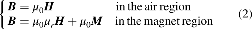
Since the outer and inner layer magnets are independent, the superposition method is used. According to (1)–(2), the Poisson and Laplace equations of each subdomain in terms of the scalar potential can be solved.

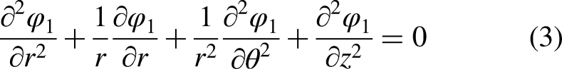
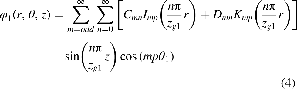
Inner Subdomain Equation in Terms of Scalar Potential

The governing Laplace equation with the scalar potential φ₁(r, θ, z) in cylindrical coordinates can be written as

\frac{\partial^{2} φ_{1}}{\partial r^{2}} + \frac{1}{r} \frac{\partial φ_{1}}{\partial r} + \frac{1}{r^{2}} \frac{\partial^{2} φ_{1}}{\partial θ^{2}} + \frac{\partial^{2} φ_{1}}{\partial z^{2}} = 0

(3)

In the inner subdomain (R_r₁< r < R_m₂ and 0 < h < h₁+ g₁), using the method of separating variables, the analytical expression of (3) is

\begin{aligned} φ_{1} (r, θ, z) = \sum_{m = o d d}^{\infty} \sum_{n = 0}^{\infty} [C_{m n} I_{m p} (\frac{n π}{z_{g 1}} r) + D_{m n} K_{m p} (\frac{n π}{z_{g 1}} r)] \\ \sin (\frac{n π}{z_{g 1}} z) \cos (m p θ_{1}) \end{aligned}

(4)

where C_mn and D_mn are undetermined coefficients, I_mp and K_mp are Bessel functions, and z_g₁= h₁+ g₁.

Middle Subdomain Equation in Terms of Scalar Potential

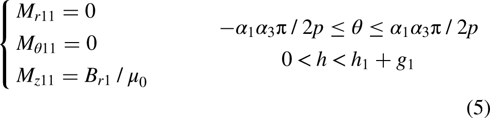
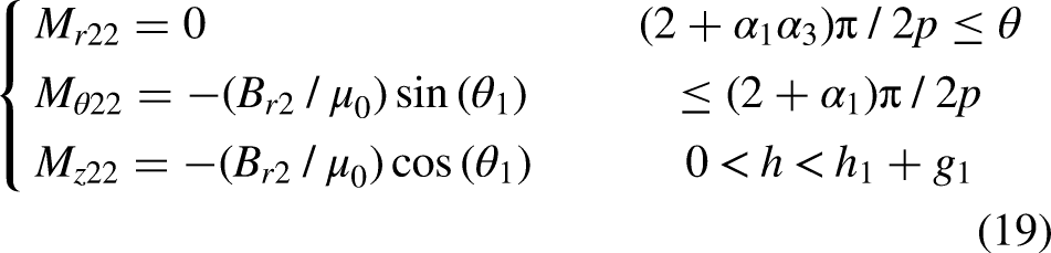
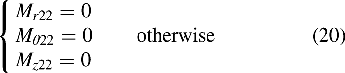
Due to the remanences of the mid-magnet and side-magnet in the middle subdomain are different, the middle subdomain is divided into magnetization systems 1 and 2, in which the magnetization M is calculated respectively.

The three magnetization components of the mid-magnet in magnetization system 1 are expressed as

\begin{aligned} {\begin{matrix} M_{r 11} = 0 \\ M_{θ 11} = 0 \\ M_{z 11} = B_{r 1} / μ_{0} \end{matrix} \begin{matrix} - α_{1} α_{3} π / 2 p \leq θ \leq α_{1} α_{3} π / 2 p \\ 0 < h < h_{1} + g_{1} \end{matrix} \end{aligned}

(5)

\begin{aligned} {\begin{matrix} M_{r 11} = 0 \\ M_{θ 11} = 0 \\ M_{z 11} = - B_{r 1} / μ_{0} \end{matrix} \begin{matrix} (2 - α_{1} α_{3}) π / 2 p \leq θ \leq (2 + α_{1} α_{3}) π / 2 p \\ 0 < h < h_{1} + g_{1} \end{matrix} \end{aligned}

(6)

{\begin{matrix} M_{r 11} = 0 \\ M_{θ 11} = 0 \\ M_{z 11} = 0 \end{matrix} otherwise

(7)

where B_r₁ is the remanence of mid-magnet, M_r₁₁, M_θ₁₁ and M_z₁₁ are the three magnetization components of the mid-magnet, p is the pole pair number.

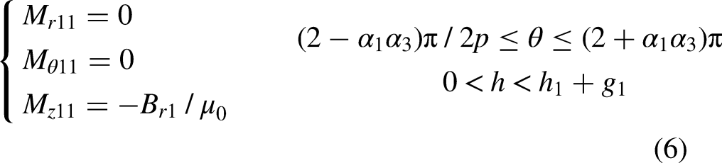
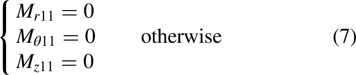
According to the mirror symmetry, the three magnetization components of the symmetric mid-magnet in magnetization system 1 can be given as

\begin{aligned} {\begin{matrix} M_{r 12} = 0 \\ M_{θ 12} = 0 \\ M_{z 12} = B_{r 1} / μ_{0} \end{matrix} \begin{matrix} - α_{1} α_{3} π / 2 p \leq θ \leq α_{1} α_{3} π / 2 p \\ 0 < h < h_{1} + g_{1} \end{matrix} \end{aligned}

(8)

\begin{aligned} {\begin{matrix} M_{r 12} = 0 \\ M_{θ 12} = 0 \\ M_{z 12} = - B_{r 1} / μ_{0} \end{matrix} \begin{matrix} (2 - α_{1} α_{3}) π / 2 p \leq θ \leq (2 + α_{1} α_{3}) π / 2 p \\ 0 < h < h_{1} + g_{1} \end{matrix} \end{aligned}

(9)

{\begin{matrix} M_{r 12} = 0 \\ M_{θ 12} = 0 \\ M_{z 12} = 0 \end{matrix} otherwise

(10)

where M_r₁₂, M_θ₁₂ and M_z₁₂ are three magnetization components of the symmetric mid-magnet.

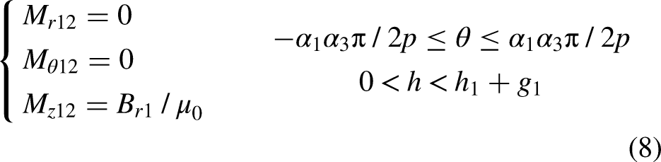
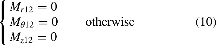
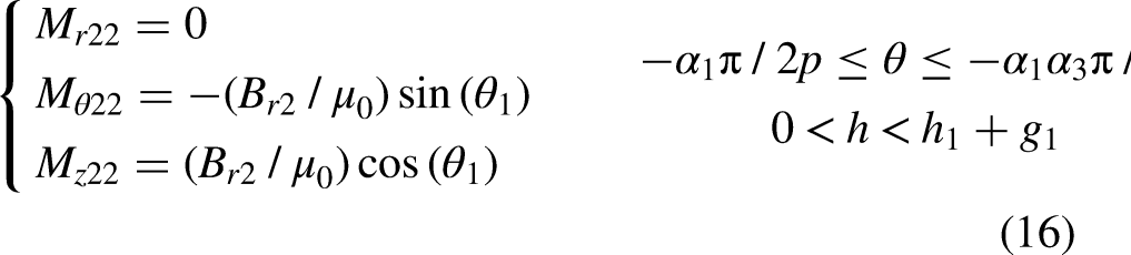
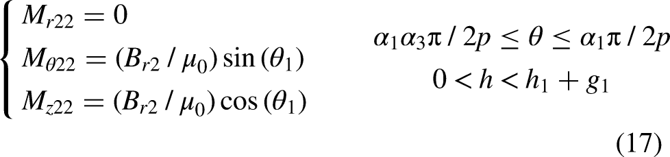
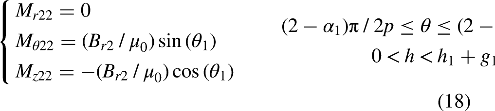
The three magnetization components of the side-magnets in magnetization system 2 is expressed as

\begin{aligned} {\begin{matrix} M_{r 21} = 0 \\ M_{θ 21} = (B_{r 2} / μ_{0}) \sin (θ_{1}) \\ M_{z 21} = (B_{r 2} / μ_{0}) \cos (θ_{1}) \end{matrix} \begin{matrix} - α_{1} π / 2 p \leq θ \leq - α_{1} α_{3} π / 2 p \\ 0 < h < h_{1} + g \end{matrix} \end{aligned}

(11)

\begin{aligned} {\begin{matrix} M_{r 21} = 0 \\ M_{θ 21} = - (B_{r 2} / μ_{0}) \sin (θ_{1}) \\ M_{z 21} = (B_{r 2} / μ_{0}) \cos (θ_{1}) \end{matrix} \begin{matrix} α_{1} α_{3} π / 2 p \leq θ \leq α_{1} π / 2 p \\ 0 < h < h_{1} + g_{1} \end{matrix} \end{aligned}

(12)

\begin{aligned} {\begin{matrix} M_{r 21} = 0 \\ M_{θ 21} = - (B_{r 2} / μ_{0}) \sin (θ_{1}) \\ M_{z 21} = - (B_{r 2} / μ_{0}) \cos (θ_{1}) \end{matrix} \begin{matrix} (2 - α_{1}) π / 2 p \leq θ \leq (2 - α_{1} α_{3}) π / 2 p \\ 0 < h < h_{1} + g_{1} \end{matrix} \end{aligned}

(13)

\begin{aligned} {\begin{matrix} M_{r 21} = 0 \\ M_{θ 21} = (B_{r 2} / μ_{0}) \sin (θ_{1}) \\ M_{z 21} = - (B_{r 2} / μ_{0}) \cos (θ_{1}) \end{matrix} \begin{matrix} (2 + α_{1} α_{3}) π / 2 p \leq θ \leq (2 + α_{1}) π / 2 p \\ 0 < h < h_{1} + g_{1} \end{matrix} \end{aligned}

(14)

{\begin{matrix} M_{r 21} = 0 \\ M_{θ 21} = 0 \\ M_{z 21} = 0 \end{matrix} otherwise

(15)

where B_r₂ is the remanence of the side-magnets, M_r₂₁, M_θ₂₁ and M_z₂₁ are three magnetization components of the side-magnets.

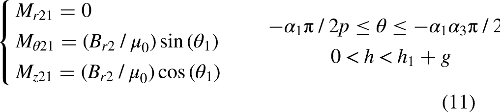
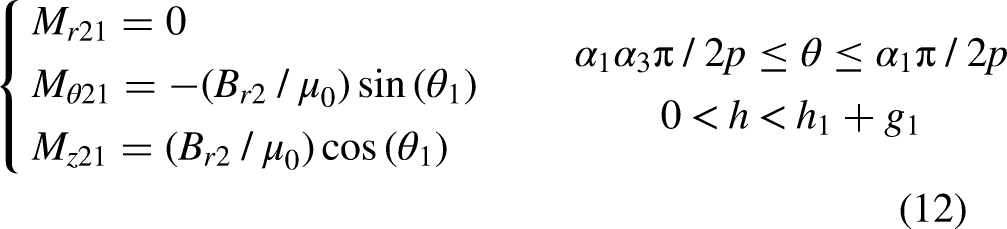
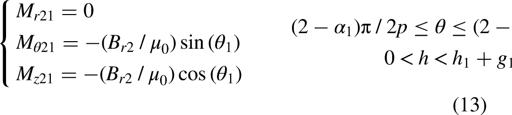
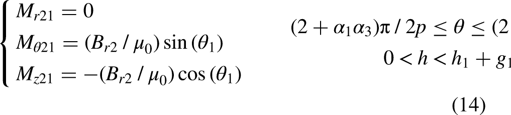
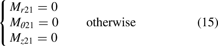
According to the mirror symmetry, the three magnetization components of the symmetric side-magnets in magnetization system 2 can be given as

\begin{aligned} {\begin{matrix} M_{r 22} = 0 \\ M_{θ 22} = - (B_{r 2} / μ_{0}) \sin (θ_{1}) \\ M_{z 22} = (B_{r 2} / μ_{0}) \cos (θ_{1}) \end{matrix} \begin{matrix} - α_{1} π / 2 p \leq θ \leq - α_{1} α_{3} π / 2 p \\ 0 < h < h_{1} + g_{1} \end{matrix} \end{aligned}

(16)

\begin{aligned} {\begin{matrix} M_{r 22} = 0 \\ M_{θ 22} = (B_{r 2} / μ_{0}) \sin (θ_{1}) \\ M_{z 22} = (B_{r 2} / μ_{0}) \cos (θ_{1}) \end{matrix} \begin{matrix} α_{1} α_{3} π / 2 p \leq θ \leq α_{1} π / 2 p \\ 0 < h < h_{1} + g_{1} \end{matrix} \end{aligned}

(17)

\begin{aligned} {\begin{matrix} M_{r 22} = 0 \\ M_{θ 22} = (B_{r 2} / μ_{0}) \sin (θ_{1}) \\ M_{z 22} = - (B_{r 2} / μ_{0}) \cos (θ_{1}) \end{matrix} \begin{matrix} (2 - α_{1}) π / 2 p \leq θ \leq (2 - α_{1} α_{3}) π / 2 p \\ 0 < h < h_{1} + g_{1} \end{matrix} \end{aligned}

(18)

\begin{aligned} {\begin{matrix} M_{r 22} = 0 \\ M_{θ 22} = - (B_{r 2} / μ_{0}) \sin (θ_{1}) \\ M_{z 22} = - (B_{r 2} / μ_{0}) \cos (θ_{1}) \end{matrix} \begin{matrix} (2 + α_{1} α_{3}) π / 2 p \leq θ \\ \leq (2 + α_{1}) π / 2 p \\ 0 < h < h_{1} + g_{1} \end{matrix} \end{aligned}

(19)

{\begin{matrix} M_{r 22} = 0 \\ M_{θ 22} = 0 \\ M_{z 22} = 0 \end{matrix} otherwise

(20)

where M_r₂₂, M_θ₂₂ and M_z₂₂ are three magnetization components of the side-magnets.

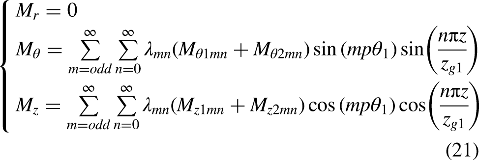
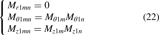
The three magnetization components of magnetization systems 1 and 2 are both decomposed by the double Fourier. The total magnetization of the middle subdomain can be derived as

{\begin{matrix} M_{r} = 0 \\ M_{θ} = \sum_{m = o d d}^{\infty} \sum_{n = 0}^{\infty} λ_{m n} (M_{θ 1 m n} + M_{θ 2 m n}) \sin (m p θ_{1}) \sin (\frac{n π z}{z_{g 1}}) \\ M_{z} = \sum_{m = o d d}^{\infty} \sum_{n = 0}^{\infty} λ_{m n} (M_{z 1 m n} + M_{z 2 m n}) \cos (m p θ_{1}) \cos (\frac{n π z}{z_{g 1}}) \end{matrix}

(21)

where

{\begin{matrix} M_{r 1 m n} = 0 \\ M_{θ 1 m n} = M_{θ 1 m} M_{θ 1 n} \\ M_{z 1 m n} = M_{z 1 m} M_{z 1 n} \end{matrix}

(22)

{\begin{matrix} M_{r 2 m n} = 0 \\ M_{θ 2 m n} = M_{θ 2 m} M_{θ 2 n} \\ M_{z 2 m n} = M_{z 2 m} M_{z 2 n} \end{matrix}

(23)

λ_{m n} = {\begin{matrix} 1 / 2 n = 0 \\ 1 n \neq 0 \end{matrix}

(24)

where T = π/p, M_r, M_θ and M_z are the magnetization components in the r, θ and z directions, respectively. M_r_1mn, M_θ_1mn and M_z_1mn are the Fourier decomposition coefficients in magnetization system 1, M_r_2mn, M_θ_2mn and M_z_2mn are the Fourier decomposition coefficients in magnetization system 2.

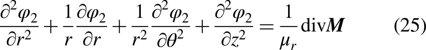
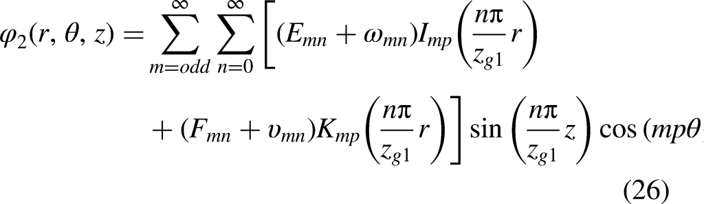
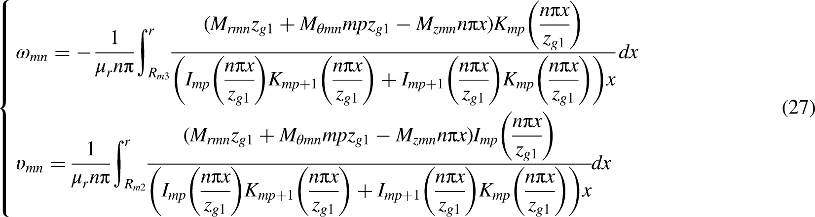
The governing Poisson equation with the scalar potential φ₂(r, θ, z) in cylindrical coordinates can be written as

\frac{\partial^{2} φ_{2}}{\partial r^{2}} + \frac{1}{r} \frac{\partial φ_{2}}{\partial r} + \frac{1}{r^{2}} \frac{\partial^{2} φ_{2}}{\partial θ^{2}} + \frac{\partial^{2} φ_{2}}{\partial z^{2}} = \frac{1}{μ_{r}} div M

(25)

In the middle subdomain (R_m₂< r < R_m₃ and 0 < h < h₁+ g₁), using the method of separating variables, the analytical expression of (25) is

\begin{aligned} φ_{2} (r, θ, z) = & \sum_{m = o d d}^{\infty} \sum_{n = 0}^{\infty} [(E_{m n} + ω_{m n}) I_{m p} (\frac{n π}{z_{g 1}} r) \\ + (F_{m n} + υ_{m n}) K_{m p} (\frac{n π}{z_{g 1}} r)] \sin (\frac{n π}{z_{g 1}} z) \cos (m p θ_{1})) \end{aligned}

(26)

where

{\begin{matrix} ω_{m n} = - \frac{1}{μ_{r} n π} \int_{R_{m 3}}^{r} \frac{(M_{r m n} z_{g 1} + M_{θ m n} m p z_{g 1} - M_{z m n} n π x) K_{m p} (\frac{n π x}{z_{g 1}})}{(I_{m p} (\frac{n π x}{z_{g 1}}) K_{m p + 1} (\frac{n π x}{z_{g 1}}) + I_{m p + 1} (\frac{n π x}{z_{g 1}}) K_{m p} (\frac{n π x}{z_{g 1}})) x} d x \\ υ_{m n} = \frac{1}{μ_{r} n π} \int_{R_{m 2}}^{r} \frac{(M_{r m n} z_{g 1} + M_{θ m n} m p z_{g 1} - M_{z m n} n π x) I_{m p} (\frac{n π x}{z_{g 1}})}{(I_{m p} (\frac{n π x}{z_{g 1}}) K_{m p + 1} (\frac{n π x}{z_{g 1}}) + I_{m p + 1} (\frac{n π x}{z_{g 1}}) K_{m p} (\frac{n π x}{z_{g 1}})) x} d x \end{matrix}

(27)

{\begin{matrix} M_{r m n} = M_{r 1 m n} + M_{r 2 m n} \\ M_{θ m n} = M_{θ 1 m n} + M_{θ 2 m n} \\ M_{z m n} = M_{z 1 m n} + M_{z 2 m n} \end{matrix}

(28)

where E_mn and F_mn are undetermined coefficients.

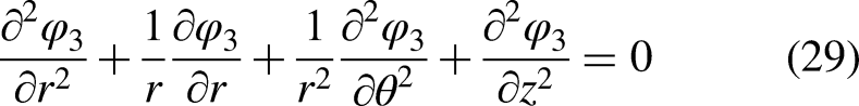
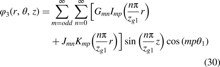
Outer Subdomain Equation in Terms of Scalar Potential

The governing Laplace equation with the scalar potential φ₃(r, θ, z) in cylindrical coordinates can be written as

\frac{\partial^{2} φ_{3}}{\partial r^{2}} + \frac{1}{r} \frac{\partial φ_{3}}{\partial r} + \frac{1}{r^{2}} \frac{\partial^{2} φ_{3}}{\partial θ^{2}} + \frac{\partial^{2} φ_{3}}{\partial z^{2}} = 0

(29)

In the outer subdomain (R_m₃< r < R_r₂ and 0 < h < h₁+ g₁), using the method of separating variables, the analytical expression of (29) is

\begin{aligned} φ_{3} (r, θ, z) = & \sum_{m = o d d}^{\infty} \sum_{n = 0}^{\infty} [G_{m n} I_{m p} (\frac{n π}{z_{g 1}} r) \\ + J_{m n} K_{m p} (\frac{n π}{z_{g 1}} r)] \sin (\frac{n π}{z_{g 1}} z) \cos (m p θ_{1}) \end{aligned}

(30)

where G_mn and J_mn are undetermined coefficients.

Determination of Equation Coefficients

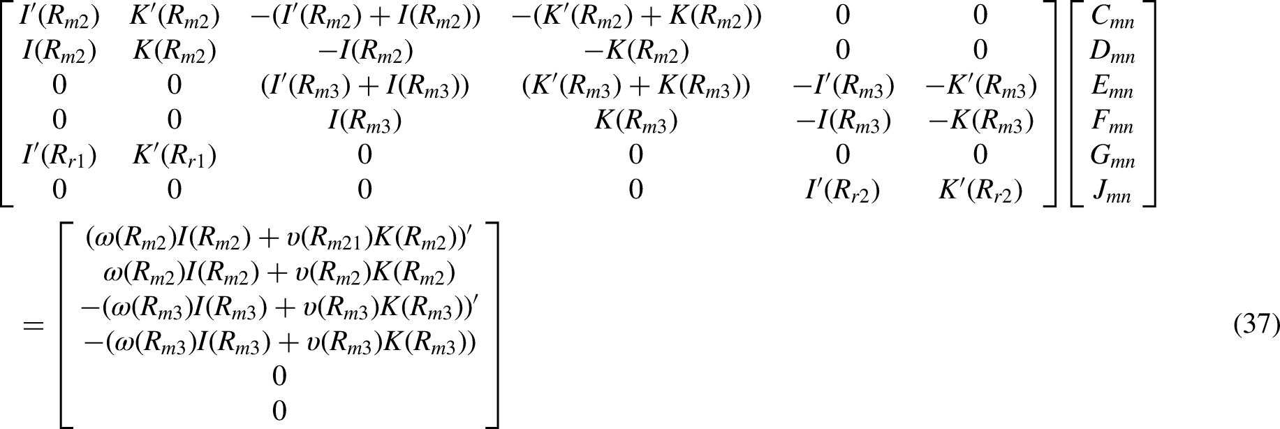
In the analytical equations with the scalar potential in different subdomains, there are six unknown coefficients C_mn, D_mn, E_mn, F_mn, G_mn and J_mn. They can be only determined by the boundary conditions.

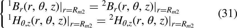
Boundary Conditions at r = R_m2

At the interface between the inner and middle subdomains (r = R_m₂), the magnetic flux density and the magnetic field strength are expressed as

{\begin{matrix} ^{1} B_{r} (r, θ, z) |_{r = R_{m 2}} =^{2} B_{r} (r, θ, z) |_{r = R_{m 2}} \\ ^{1} H_{θ, z} (r, θ, z) |_{r = R_{m 2}} =^{2} H_{θ, z} (r, θ, z) |_{r = R_{m 2}} \end{matrix}

(31)

where ¹B_r(r, θ, z) and ²B_r(r, θ, z) are the magnetic flux densities with the radial components, ¹H_θ,z(r, θ, z) and ²H_θ,z(r, θ, z) are the magnetic field strengths with the circumferential and axial components, in two subdomains, respectively.

According to (29), substituting (4), (25) into (1)–(2), the equations can be written as

{\begin{matrix} I^{'} (R_{m 2}) C_{m n} + K^{'} (R_{m 2}) D_{m n} - (I^{'} (R_{m 2}) + I (R_{m 2})) E_{m n} - (K^{'} (R_{m 2}) + K (R_{m 2})) F_{m n} = (ω (R_{m 2}) I (R_{m 2}) + υ (R_{m 2}) K (R_{m 2}))^{'} \\ I (R_{m 2}) C_{m n} + K (R_{m 2}) D_{m n} - I (R_{m 2}) E_{m n} - K (R_{m 2}) F_{m n} = ω (R_{m 2}) I (R_{m 2}) + υ (R_{m 2}) K (R_{m 2}) \end{matrix}

(32)

where I′ and K′ are the derivatives of Bessel functions I and K, respectively.

Boundary Conditions at r = R_m3

At the interface between the middle and outer subdomains (r = R_m₃), the magnetic flux density and the magnetic field strength are satisfied as

{\begin{matrix} ^{2} B_{r} (r, θ, z) |_{r = R_{m 3}} =^{3} B_{r} (r, θ, z) |_{r = R_{m 3}} \\ ^{2} H_{θ, z} (r, θ, z) |_{r = R_{m 3}} =^{3} H_{θ, z} (r, θ, z) |_{r = R_{m 3}} \end{matrix}

(33)

where ³B_r(r, θ, z) is the magnetic flux density with the radial components, and ³H_θ,z(r, θ, z) is the magnetic field strength with the circumferential and axial components.

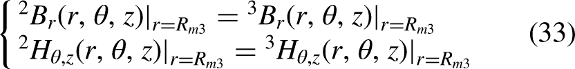
According to (31), substituting (25), (28) into (1)–(2), the equations can be solved as

{\begin{matrix} (I^{'} (R_{m 3}) + I (R_{m 3})) E_{m n} + (K^{'} (R_{m 3}) + K (R_{m 3})) F_{m n} - I^{'} (R_{m 3}) G_{m n} - K^{'} (R_{m 3}) J_{m n} = - (ω (R_{m 3}) I (R_{m 3}) + υ (R_{m 3}) K (R_{m 3}))^{'} \\ I (R_{m 3}) E_{m n} + K (R_{m 3}) F_{m n} - I (R_{m 3}) G_{m n} - K (R_{m 3}) J_{m n} = - (ω (R_{m 3}) I (R_{m 3}) + υ (R_{m 3}) K (R_{m 3})) \end{matrix}

(34)

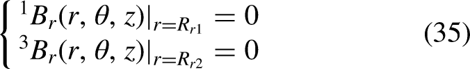
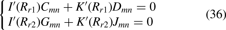
Boundary Conditions at r = R_r1 and r = R_r2

At the interfaces between the inner/outer subdomains and the air (r = R_r₁ and r = R_r₂), the radial component of the flux density is zero, i.e.,

{\begin{matrix} ^{1} B_{r} (r, θ, z) |_{r = R_{r 1}} = 0 \\ ^{3} B_{r} (r, θ, z) |_{r = R_{r 2}} = 0 \end{matrix}

(35)

According to (33), substituting (4), (28) into (1)–(2), the equations can be solved as

{\begin{matrix} I^{'} (R_{r 1}) C_{m n} + K^{'} (R_{r 1}) D_{m n} = 0 \\ I^{'} (R_{r 2}) G_{m n} + K^{'} (R_{r 2}) J_{m n} = 0 \end{matrix}

(36)

According to (30), (32) and (34), the matrix equation with six coefficients C_mn, D_mn, E_mn, F_mn, G_mn and J_mn can be written as

[\begin{matrix} I^{'} (R_{m 2}) & K^{'} (R_{m 2}) & - (I^{'} (R_{m 2}) + I (R_{m 2})) & - (K^{'} (R_{m 2}) + K (R_{m 2})) & 0 & 0 \\ I (R_{m 2}) & K (R_{m 2}) & - I (R_{m 2}) & - K (R_{m 2}) & 0 & 0 \\ 0 & 0 & (I^{'} (R_{m 3}) + I (R_{m 3})) & (K^{'} (R_{m 3}) + K (R_{m 3})) & - I^{'} (R_{m 3}) & - K^{'} (R_{m 3}) \\ 0 & 0 & I (R_{m 3}) & K (R_{m 3}) & - I (R_{m 3}) & - K (R_{m 3}) \\ I^{'} (R_{r 1}) & K^{'} (R_{r 1}) & 0 & 0 & 0 & 0 \\ 0 & 0 & 0 & 0 & I^{'} (R_{r 2}) & K^{'} (R_{r 2}) \end{matrix}] [\begin{matrix} C_{m n} \\ D_{m n} \\ E_{m n} \\ F_{m n} \\ G_{m n} \\ J_{m n} \end{matrix}] = [\begin{matrix} (ω (R_{m 2}) I (R_{m 2}) + υ (R_{m 21}) K (R_{m 2}))^{'} \\ ω (R_{m 2}) I (R_{m 2}) + υ (R_{m 2}) K (R_{m 2}) \\ - (ω (R_{m 3}) I (R_{m 3}) + υ (R_{m 3}) K (R_{m 3}))^{'} \\ - (ω (R_{m 3}) I (R_{m 3}) + υ (R_{m 3}) K (R_{m 3})) \\ 0 \\ 0 \end{matrix}]

(37)

By solving (35), the unknown coefficients can be obtained.

Analytical Performance of Slotted AFM

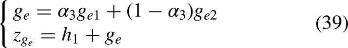
Based on the analytically obtained slotless magnetic field, considering the slotting effect, a Carter's coefficient is used for calculation of equivalent airgap length.

The equivalent airgap lengths in different paths are calculated as

{\begin{matrix} g_{e 1} = C_{s} g_{1} \\ g_{e 2} = C_{s} g \end{matrix}

(38)

where C_s is the Carter's coefficient, g₁ and g_e₁ are the actual and equivalent airgap lengths of the side-magnets, g and g_e₂ are the actual and equivalent airgap lengths of the mid-magnet.

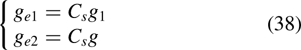
The total equivalent airgap length g_e is

{\begin{matrix} g_{e} = α_{3} g_{e 1} + (1 - α_{3}) g_{e 2} \\ z_{g_{e}} = h_{1} + g_{e} \end{matrix}

(39)

The axial component of the flux density is

\begin{aligned} B_{z} = & μ_{0} \sum_{m = o d d}^{\infty} \sum_{n = 0}^{\infty} \frac{{(- 1)}^{n} n π}{z_{g_{e}}} [(E_{m n} + ω_{m n}) I_{m p} (\frac{n π r}{z_{g_{e}}}) \\ + (F_{m n} + υ_{m n}) K_{m p} (\frac{n π r}{z_{g_{e}}})] \cos (m p θ_{1}) \end{aligned}

(40)

The flux linkage of one coil is

\begin{aligned} Ψ = & \frac{2 N μ_{0} π}{p z_{g_{e}}} \int_{R_{m 2}}^{R_{m 3}} [(E_{m n} + ω_{m n}) I_{m p} (\frac{n π r}{z_{g_{e}}}) + (F_{m n} + υ_{m n}) \\ K_{m p} (\frac{n π r}{z_{g_{e}}})] r d r \cdot \sum_{m = o d d}^{\infty} \sum_{n = 0}^{\infty} \frac{{(- 1)}^{n} n}{m} \cos (m p (- ω_{r} t + α_{c p} (j - 1))) \sin \frac{m p α_{c p}}{2} \end{aligned}

(41)

where N is the number of coil turns, and α_cp is the pitch angle of the coil.

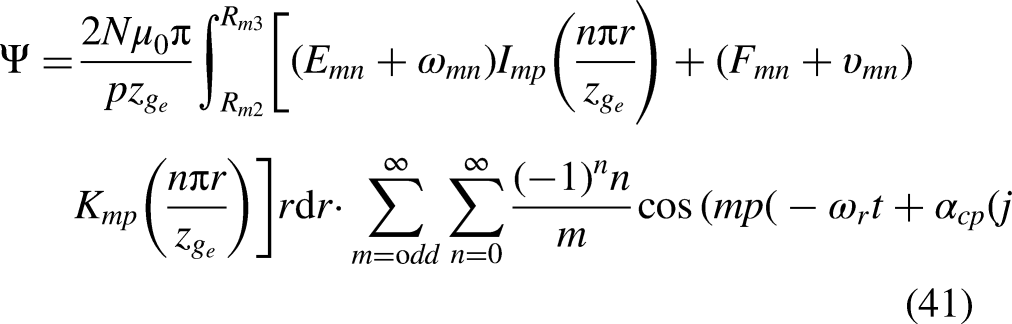
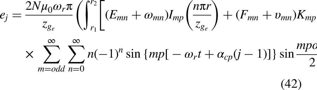
The back electromotive force (EMF) of each phase in the j-th coil is calculated as

e_{j} = \frac{2 N μ_{0} ω_{r} π}{z_{g_{e}}} (\int_{r_{1}}^{r_{2}} [(E_{m n} + ω_{m n}) I_{m p} (\frac{n π r}{z_{g_{e}}}) + (F_{m n} + υ_{m n}) K_{m p} (\frac{n π r}{z_{g_{e}}})] r d r) \sum_{m = o d d}^{\infty} \sum_{n = 0}^{\infty} n {(- 1)}^{n} \sin {m p [- ω_{r} t + α_{c p} (j - 1)]} \sin \frac{m p α_{c p}}{2}

(42)

The proposed AFM has a dual-stator configuration and the stator winding distribution is shown in Figure 5.

Figure 5.

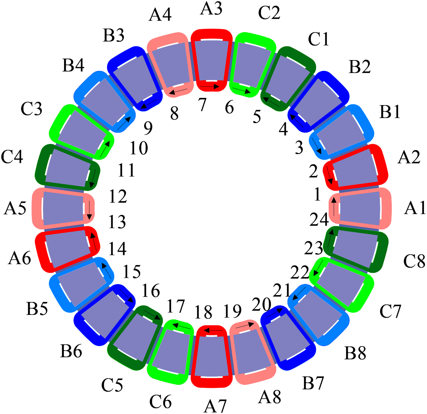
Coil distribution of a 20-pole/24-slot AFM.

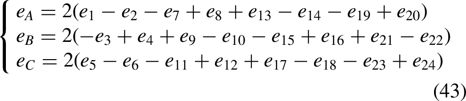
According to the 24-slot stator, three back electromotive forces can be obtained as

{\begin{matrix} e_{A} = 2 (e_{1} - e_{2} - e_{7} + e_{8} + e_{13} - e_{14} - e_{19} + e_{20}) \\ e_{B} = 2 (- e_{3} + e_{4} + e_{9} - e_{10} - e_{15} + e_{16} + e_{21} - e_{22}) \\ e_{C} = 2 (e_{5} - e_{6} - e_{11} + e_{12} + e_{17} - e_{18} - e_{23} + e_{24}) \end{matrix}

(43)

The electromagnetic torque can be analytically calculated by

T_{e} = \frac{e_{A} i_{A} + e_{B} i_{B} + e_{C} i_{C}}{ω_{r}}

(44)

where i_A, i_B and i_C are three phase currents, and ω_r is the rotational angular speed.

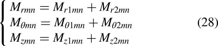
It is noted that the foregoing analytical process is applied for the outer layer magnets. Since the analytical process for the inner layer magnets is similar, it is not presented for conciseness. Using the superposition method, these electromagnetic parameters for the proposed AFM can be analytically obtained.

Analytical Result Comparison and Verification

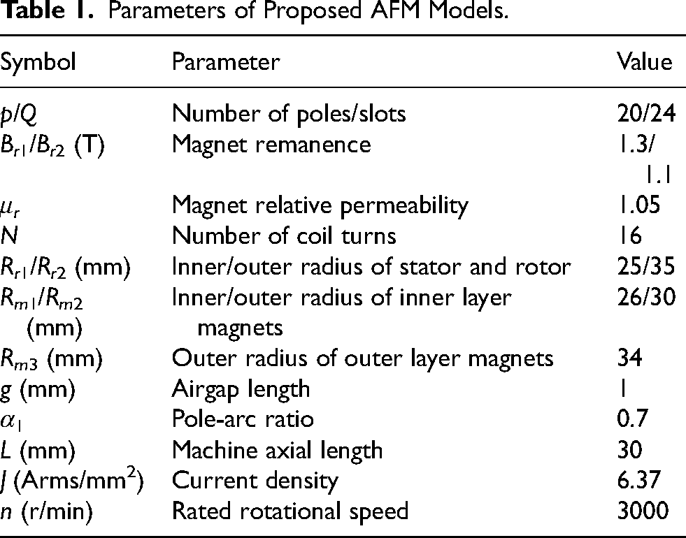
Using the analytical equations presented in Sections 3 to 5, the performances of the AFMs with surface-mounted non-layered/layered and segmented Halbach magnets are compared. Table 1 gives the main parameters of the AFMs. For the fair comparison, the remanence per unit volume of the magnet usage is the same for all the compared AFMs.

Table 1.

Parameters of Proposed AFM Models.

Symbol	Parameter	Value
p/Q	Number of poles/slots	20/24
B_r₁/B_r₂ (T)	Magnet remanence	1.3/1.1
μ_r	Magnet relative permeability	1.05
N	Number of coil turns	16
R_r₁/R_r₂ (mm)	Inner/outer radius of stator and rotor	25/35
R_m₁/R_m₂ (mm)	Inner/outer radius of inner layer magnets	26/30
R_m₃ (mm)	Outer radius of outer layer magnets	34
g (mm)	Airgap length	1
α ₁	Pole-arc ratio	0.7
L (mm)	Machine axial length	30
J (Arms/mm²)	Current density	6.37
n (r/min)	Rated rotational speed	3000

For the proposed Machine IV, the magnetization angle θ₁ and the ratio α₃ of the outer layer magnets, the magnetization angle θ₂ and the ratio α₂ of the inner layer magnets influence the electromagnetic torque. These four parameters are chosen as the optimization variables. The optimization object is the maximum electromagnetic torque. The average electromagnetic torque against θ₁ and α₃, θ₂ and α₂ is shown in Figure 6. It can be easily obtained that the optimized results are θ₁= 29°, α₃= 0.54, θ₂= 34° and α₂= 0.48.

Figure 6.

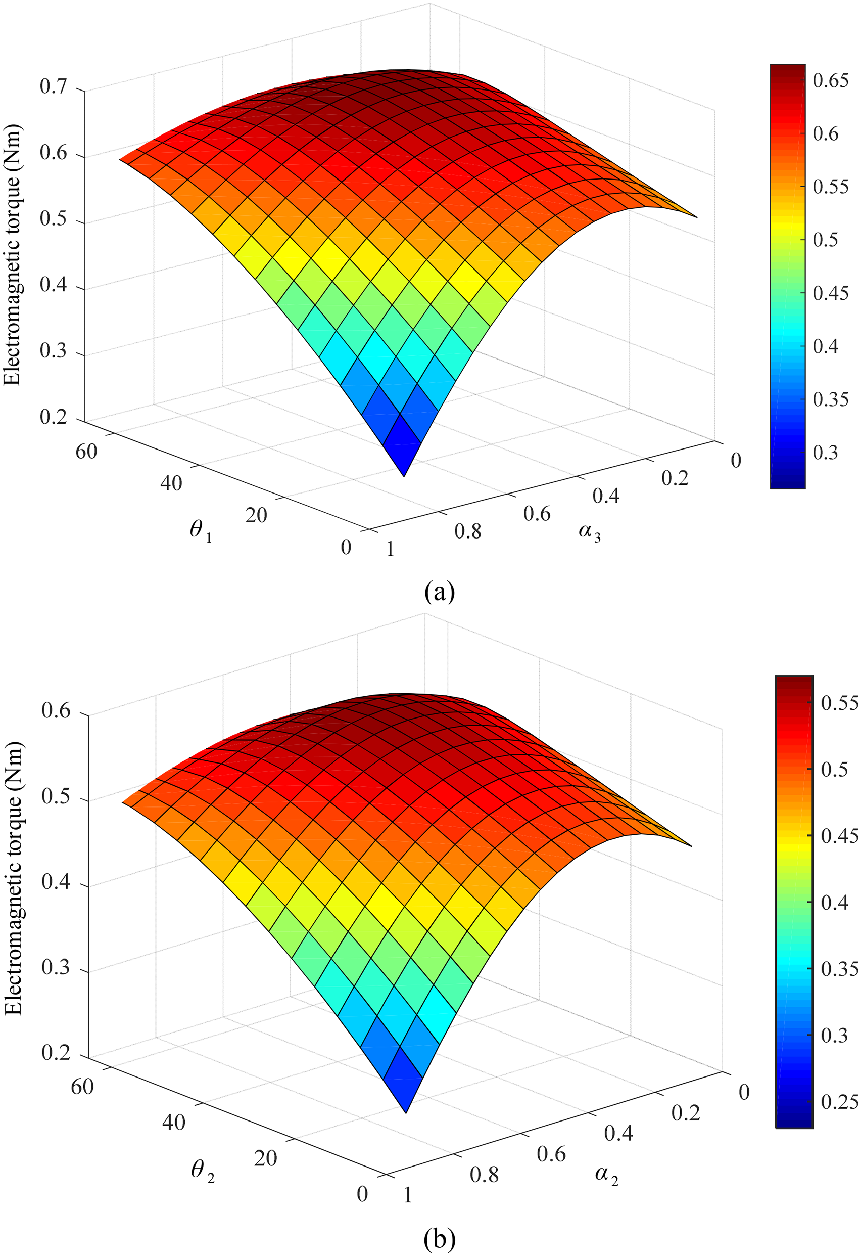
Analytical electromagnetic torque against different variables for proposed machine IV with outer/inner magnets. (a) Torque against with θ₁ and α₃ for outer layer magnets. (b) Torque against with θ₂ and α₂ for inner layer magnets.

Figure 7(a) compares the 3-D analytically predicted airgap flux density waveforms of four AFMs. It can be clearly seen that the proposed Machine IV has the best waveform with the maximum value 1.29 T and the proposed Machine III has the second best waveform. Figure 7(b) shows the comparison of the 3-D analytical and FEA airgap flux density waveforms of proposed optimized Machine IV. It can be clearly observed that the two waveforms of the optimized 3-D analytical and FEA models for proposed Machine IV are well matched.

Figure 7.

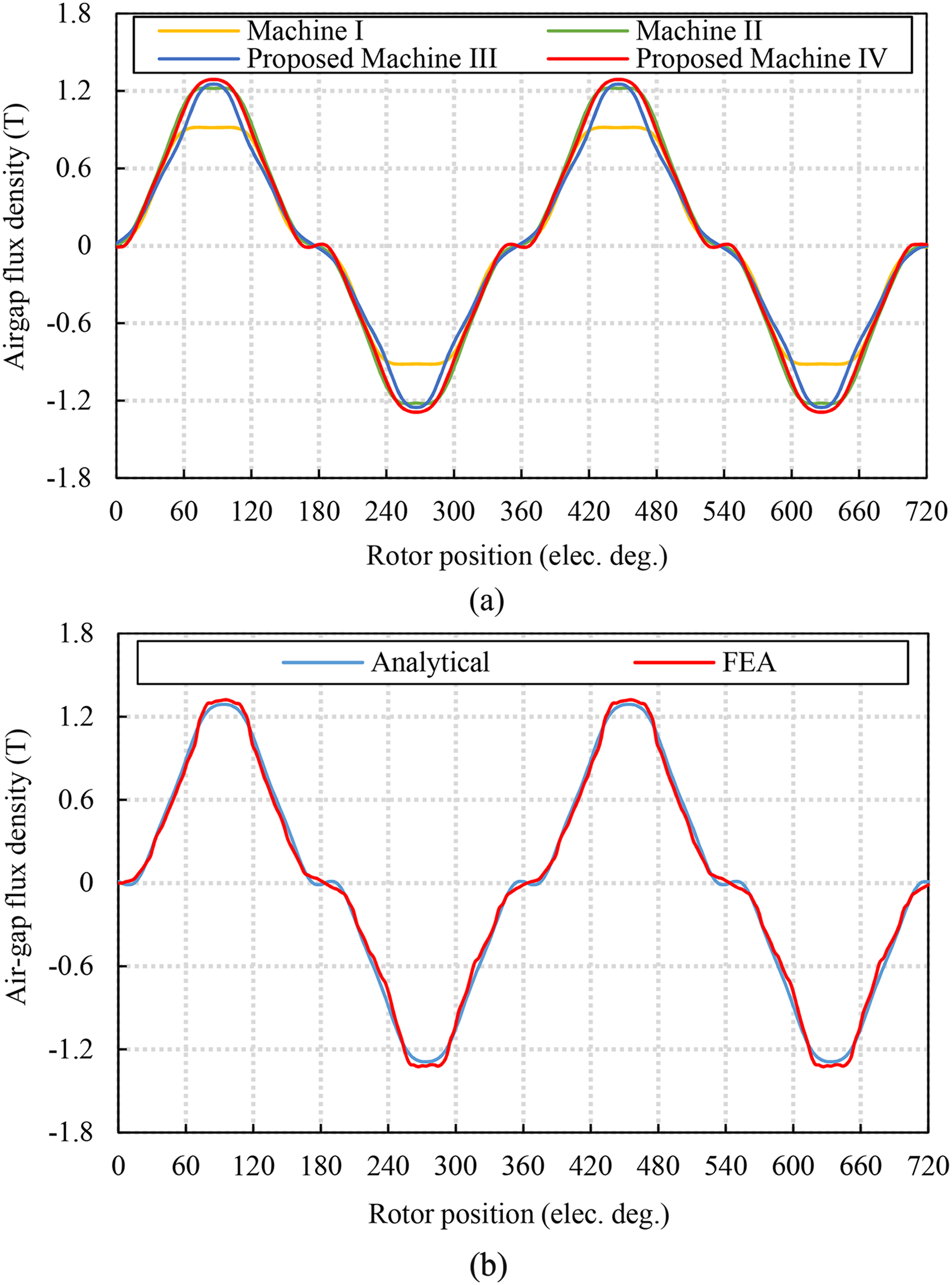
Comparison of airgap flux density waveforms. (a) Comparison of 3-D analytically predicted flux density waveforms of four AFMs. (b) Comparison of 3-D analytical and FEA flux density waveforms of proposed optimized Machine IV.

Figure 8(a) shows the analytical comparison of phase back-EMF waveforms of four AFMs. The maximum waveform values for Machines I, II, III and IV are 32.7, 37.3, 38.4 and 39.13 V, respectively. Figure 8(b) shows the corresponding harmonic comparison of four back-EMF waveforms. The fundamental component values of four AFMs are 31.15, 34.42, 35.54 and 36.86 V, respectively. It can be clearly seen that the proposed Machine IV has the best fundamental value and the proposed Machine III has the second best fundamental value. As shown in Figure 8(c), there is an excellent agreement between the 3-D analytical and FEA back-EMF waveforms of proposed optimized Machine IV.

Figure 8.

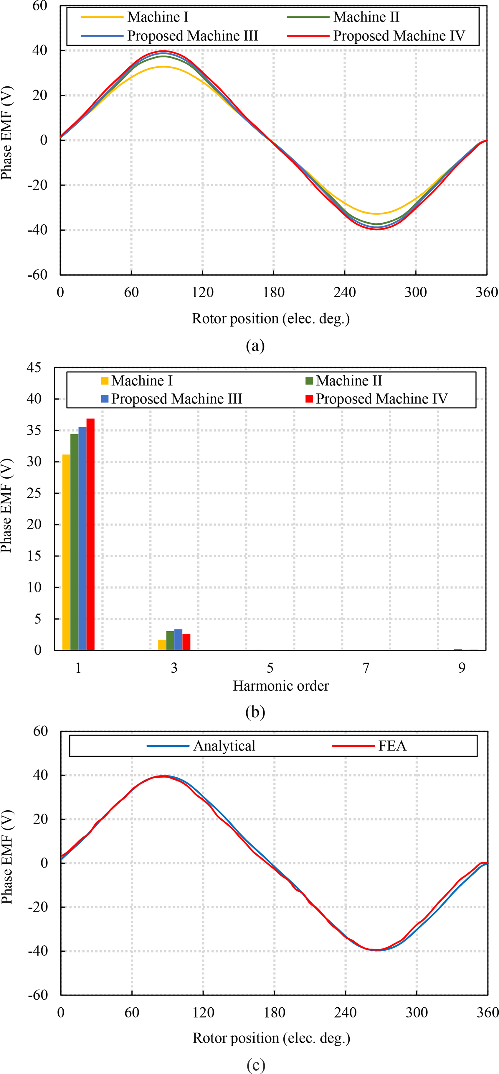
Comparison of phase back-EMF waveforms. (a) Comparison of 3-D analytical back-EMF waveforms of four AFMs. (b) Comparison of harmonics of back-EMF waveforms of four AFMs. (c) Comparison of 3-D analytical and FEA back-EMF waveforms of proposed optimized Machine IV.

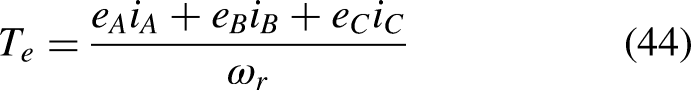
Electromagnetic torque is one critical output properties in the motor operation. Figure 9(a) shows the analytical electromagnetic torque waveforms of the four compared AFMs. The average electromagnetic torque values are 1.047, 1.183, 1.208 and 1.227 Nm, respectively. It can be clearly seen that the proposed Machine IV has the best torque value and the proposed Machine III has the second best torque value. Figure 9(b) shows that an excellent agreement is achieved between the 3-D analytical and FEA torque waveforms of proposed optimized Machine IV.

Figure 9.

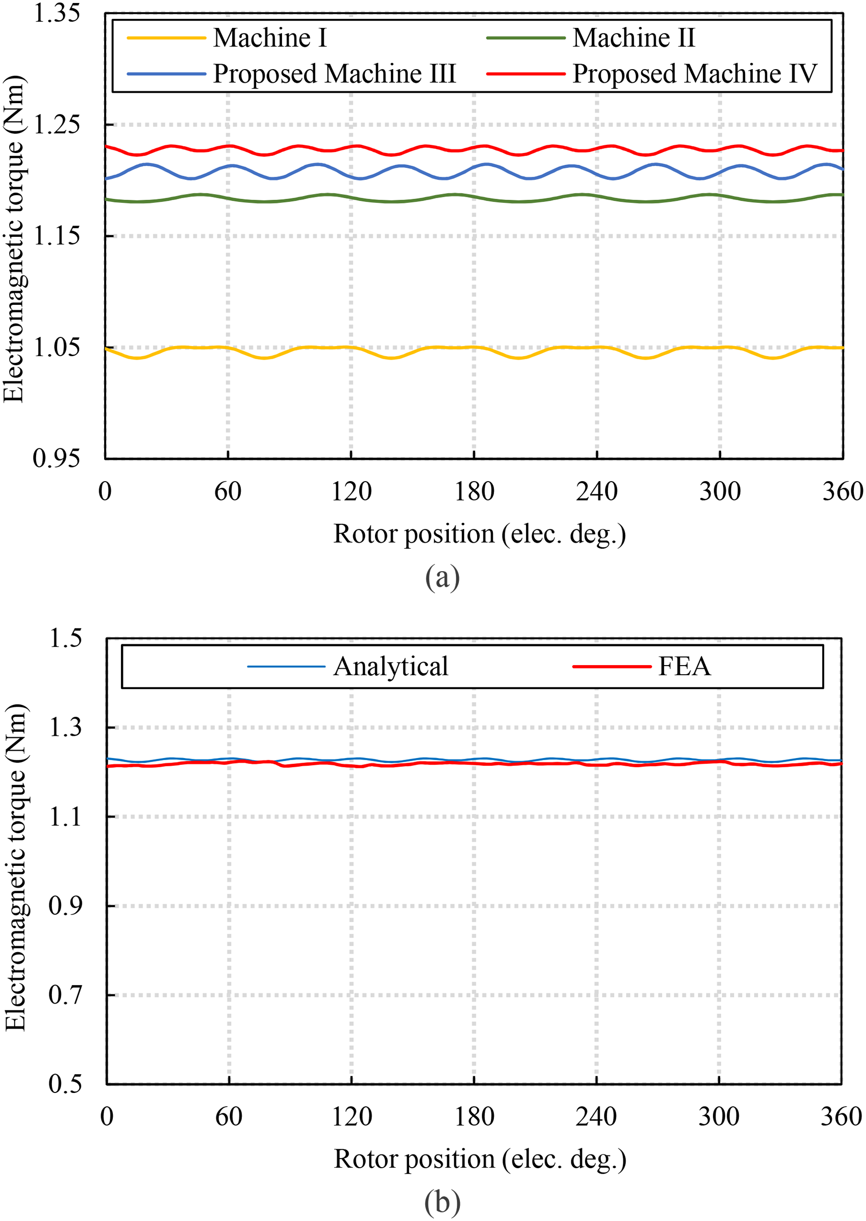
Comparison of electromagnetic torque waveforms. (a) 3-D analytical torque waveform comparison between four AFMs. (b) Comparison of 3-D analytical and FEA torque waveforms of proposed optimized Machine IV with radially layered unequal-height Halbach magnets.

Conclusion

The 3-D linear analytical models have been compared for AFMs with surface-mounted non-layered/layered and segmented Halbach magnets. Using the 3-D analytical subdomain method, using the superposition method, the 3-D magnetic field in the AFM with the layered Halbach arrays has been solved and analyzed. In addition, the four magnet parameters are chosen as the optimization variables, the electromagnetic torque has been optimized. The analytical correctness of the proposed 3-D model with proposed optimized Machine IV is verified with the results of FEA. It is well demonstrated that with the same magnet cost, the optimized AFM with the radially layered unequal-height Halbach magnets exhibits the best electromagnetic performance and that with the axially layered unequal-height Halbach magnets exhibits the second best one. The 3-D analytical performances of the layered AFMs are obviously better than those of the non-layered ones.

Footnotes

Acknowledgements

This work was supported by the Anhui Provincial Natural Science Foundation under Grant 2008085ME179 and the 111 Project under Grant BP0719039.

ORCID iD

Youyuan Ni

Funding

The authors received no financial support for the research, authorship, and/or publication of this article.

Declaration of Conflicting Interests

The authors declared no potential conflicts of interest with respect to the research, authorship, and/or publication of this article.

References

Geng

(2022). A new flux-concentrating rotor of double stator and single rotor axial flux permanent magnet machine for electric vehicle traction application. 2022 IEEE Vehicle Power and Propulsion Conference (VPPC) (pp. 1–6), Merced, CA, USA.

Geng

Zhang

(2018). Analysis and implementation of new ironless stator axial-flux permanent magnet machine with concentrated nonoverlapping windings. IEEE Transactions on Energy Conversion, 33(3), 1274–1284. https://doi.org/10.1109/TEC.2018.2799172

Gieras

J. F.

Wang

R.-J.

Kamper

(2008). Axial flux permanent magnet brushless machines (2nd ed.). Springer-Verlag.

Habib

Zainuria

M. A. A. M.

Che

H. S.

Ibrahim

A. A.

(2022). An appreciation of using Halbach magnets array in axial flux permanent magnet machines. 2022 IEEE Industrial Electronics and Applications Conference (IEACon) (pp. 94–98), Kuala Lumpur, Malaysia.

Jin, P., Yuan, Y., Minyi, J., Shuhua, F., Heyun, L., & Yang, H., (2014). 3-D Analytical magnetic field analysis of axial flux permanent-magnet machine. IEEE Transactions on Magnetics, 50(11), 1–4. https://doi.org/10.1109/TMAG.2014.2323573

Jin

Yuan

, Fang, S., Lin, H., & Ho, S. L. (2015). Analysis of axial-flux Halbach permanent-magnet machine. IEEE Transactions on Magnetics, 51(11), 1–4.

Kahourzade, S., Mahmoudi, A., Hew, W., & Nasir Uddin, M. (2014). A comprehensive review of axial-flux permanent-magnet machines. Canadian Journal of Electrical and Computer Engineering, 37(1), 19–33. https://doi.org/10.1109/CJECE.2014.2309322

Lu, Y., Kai, Y., Sun, S., Luo, Y., Fei, X., & Cheng, L. (2024). Study on the influence of a combined-Halbach array for the axial flux permanent magnet electrical machine with yokeless and segmented armature. IEEE Transactions on Magnetics, 60(3), 1–5. https://doi.org/10.1109/TMAG.2023.3287708

Nishanth

Verdeghem

J. V.

Severson

E. L.

(2021). Recent advances in analysis and design of axial flux permanent magnet electric machines. 2021 IEEE Energy Conversion Congress and Exposition (ECCE) (pp. 3745–3752), Vancouver, BC, Canada.

10.

Okita

Harada

(2023). 3-D Analytical model of axial-flux permanent magnet machine with segmented multipole-Halbach array. IEEE Access, 11, 2078–2091. https://doi.org/10.1109/ACCESS.2022.3233922

11.

Sun

Jiang

Yang

(2020). Comparison of a multi-stage axial flux permanent magnet machine with different stator core materials. IEEE Transactions on Applied Superconductivity, 30(4), 1–6. https://doi.org/10.1109/TASC.2020.2990761

12.

Sun, M. C., Tang, R. Y., Han, X. Y., & Tong, W. (2018). Analysis and modeling for open circuit air gap magnetic field prediction in axial flux permanent magnet machines. Proceedings of the CSEE, 38(5), 1525–1533. https://doi.org/10.13334/j.0258-8013.pcsee.170505

13.

Wang, X., Zhao, X., Gao, P., & Li, T.Y. (2021). A new parallel magnetic circuit axial flux permanent magnet in-wheel machine. 2021 24th International Conference on Electrical Machines and Systems (ICEMS) (pp. 1107–1111), Gyeongju, Korea.

14.

Yang

(2021). One adopts trapezoidal permanent magnet block array type novel axial flux stator coreless permanent magnet machine. 2021 24th International Conference on Electrical Machines and Systems (ICEMS) (pp. 1133–1136), Gyeongju, Korea.

15.

Zerioul, A., Hadjout, L., Ouazir, Y., Bensaidane, H., Benbekai, A., & Chaouch, O. (2018). 3D Analytical model to compute the electromagnetic torque of axial flux magnetic coupler with a rectangular-shaped magnet. 2018 International Conference on Electrical Sciences and Technologies in Maghreb (CISTEM) (pp. 1–4), Algiers, Algeria.

16.

Zhang

Wang

Geng

(2020). Design and optimization of Halbach-array PM rotor for high-speed axial-flux permanent magnet machine with ironless stator. IEEE Transactions on Industrial Electronics, 67(9), 7269–7279. https://doi.org/10.1109/TIE.2019.2944033

17.

Zhao

Lipo

T. A.

Kwon

B.-I.

(2014). A novel dual-stator axial-flux spoke-type permanent magnet vernier machine for direct-drive applications. IEEE Transactions on Magnetics, 50(11), 1–4. https://doi.org/10.1109/TMAG.2014.2329861

3-D Analytical Comparison of Axial Flux Machines With Layered and Segmented Halbach Magnets

Abstract

Keywords

Introduction

AFM Physical Model

General Solution Equations for Subdomains

Inner Subdomain Equation in Terms of Scalar Potential

Middle Subdomain Equation in Terms of Scalar Potential

Outer Subdomain Equation in Terms of Scalar Potential

Determination of Equation Coefficients

Boundary Conditions at r = Rm2

Boundary Conditions at r = Rm3

Boundary Conditions at r = Rr1 and r = Rr2

Analytical Performance of Slotted AFM

Analytical Result Comparison and Verification

Conclusion

Footnotes

Acknowledgements

ORCID iD

Funding

Declaration of Conflicting Interests

References

Boundary Conditions at r = R_m2

Boundary Conditions at r = R_m3

Boundary Conditions at r = R_r1 and r = R_r2