Classifying cognitive impairment based on FDG-PET and combined T1-MRI and rs-fMRI: An ADNI study

Abstract

Background

Mild cognitive impairment (MCI) refers to a memory impairment among non-demented adults. It is a condition that increases the risk of dementia, notably due to Alzheimer's disease (AD). MCI is heterogeneous and there is a need for novel diagnostic approaches. Fluorodeoxyglucose positron emission tomography (FDG-PET) imaging provides robust AD biomarker characteristics, while anatomical and functional magnetic resonance imaging (MRI) offer complementary information.

Objective

Classify MCI and cognitively normal (CN) adults using FDG-PET images; predict individuals with MCI that convert to AD dementia; determine if MRI can achieve comparable performance to FDG-PET classification.

Methods

Four ADNI cohorts were created. Cohort 1: 805 participants (MCI n = 455; CN n = 350) that underwent FDG-PET. FDG-PET images were inputs to a one-channel 3-dimensional (3D) DenseNet deep learning model. Cohort 2: 348 participants (MCI n = 174; CN n = 174) with MRI and functional MRI. Cohort 3: overlapping cases from cohorts 1 and 2 (MCI n = 70; CN n = 70). Cohort 4: 336 participants (MCI-converters n = 168; MCI-stable n = 168) with FDG-PET from cohort 1. The one/two-channel models’ inputs were T1-weighted MRI and/or amplitude of low-frequency fluctuations images, with classification metrics evaluated through 10-fold cross-validation.

Results

The FDG-PET model achieved 88.02%±3.82 accuracy for MCI versus CN classification, with 88.70%±4.70 sensitivity and 87.14%±5.03 specificity. Neither MRI model outperformed the FDG-PET model, as the highest MRI-based accuracy was 76.86%±1.95. The FDG-PET model achieved 63.23%±4.68 accuracy in classifying MCI-converters versus MCI-stable.

Conclusions

FDG-PET images produced the highest accuracy in classifying MCI versus CN. While MRI-based approaches were inferior to FDG-PET, multi-contrast MRI still offers value for neurodegeneration classification.

Keywords

Alzheimer's disease artificial intelligence classification deep learning FDG-PET mild cognitive impairment MRI rs-fMRI

Introduction

Mild cognitive impairment (MCI) is a clinically defined condition initially identified in non-demented adults with memory impairment and is often a premorbid condition in advance of a dementia diagnosis.^1,2 MCI involves noticeable cognitive decline, especially in memory, which exceeds typical age-related changes but does not significantly disrupt daily activities. It can be amnestic, primarily affecting memory, or non-amnestic, and impact other cognitive functions. Individuals with MCI may develop neurodegenerative conditions such as frontotemporal lobar degeneration, or limbic-predominant age-related TDP-43 encephalopathy. Some individuals may remain stable or even experience cognitive improvement over time.³ MCI is estimated to double from 12.23 million to 21.55 million in the United States between 2020 and 2060.⁴ The MCI to Alzheimer's disease (AD) related dementia conversion rate is reported as 10 to 15% annually, with roughly 80% of MCI patients convert to dementia over 6 years of follow-up.⁵ There are biological sources of heterogeneity that make the classification of MCI and cognitive normal (CN) difficult.⁶

The Mini-Mental State Examination (MMSE) is a commonly used clinical tool to help with MCI diagnosis;⁷ however, it has limitations because the score on this test is influenced by several factors, such as education and cultural differences.⁸ Positron emission tomography (PET) imaging is an essential component to diagnosing AD. ¹⁸F-fluorodeoxyglucose-PET (FDG-PET) provides an in vivo metabolic imaging contrast of glucose uptake.

Sources of MCI heterogeneity include neurovascular alterations and highlight the need for imaging-based phenotypes to characterize the diverse clinical symptomatology and/or progression patterns.^9,10 Amyloid and tau PET neuroimaging can be used individually or in combination to detect amyloid-β (Aβ) or tau protein accumulation in association with MCI and AD.^11,12 However, despite its diagnostic utility, amyloid PET can be cost-prohibitive,¹³ and tau PET currently has limited approval worldwide.¹⁴ These challenges make widespread clinical application difficult and highlight the need for more accessible diagnostic methods. Structural T1-weighted (T1) MRI is useful in AD by providing complementary soft-tissue contrast information.¹⁵ Resting-state functional MRI (rs-fMRI) is added to an MRI protocol to provide spontaneous brain activity from blood oxygenation level-dependent (BOLD) imaging contrast. rs-fMRI reveals altered connectivity in MCI and AD, specifically in the default mode network, basal ganglia network, sensorimotor network, and dorsal attention network.^16–18 MCI versus CN differences are reported based on T1 images¹⁹ as well as inherent sources of fMRI variability.²⁰

Deep learning is a branch of machine learning that is well suited to integrate spatial features to produce synthesized images, segmentation, or classification.²¹ Convolutional neural networks (CNN) are increasingly used, and a 3-dimensional (3D) network incorporates spatial information contained in the whole brain image, such as T1 used to classify CN, MCI, or AD.²² Wang and Lim used a “zoom-in” deep learning model to classify AD, MCI, and CN based on rs-fMRI.²³ Singh et al. used a CNN to classify MCI versus CN based on FDG-PET images.²⁴ The findings revealed high classification accuracy by applying dimensionality reduction techniques, outperforming traditional machine learning methods. Combining features from PET and MRI can further improve MCI versus AD classification performance, as illustrated by Odusami et al.²⁵ Deep learning has advanced in the area of dementia classification through the use of FDG-PET. Etminani et al. developed a 3D deep learning model to predict the diagnosis of dementia with Lewy bodies, AD, and MCI using brain FDG-PET.²⁶ Complex neurodegenerative disorders were classified in a robust manner, as this approach was able to differentiate between such conditions. Meanwhile, Rogeau et al. applied a 3D CNN to classify individuals as AD, frontotemporal dementia, or CN categories given brain FDG-PET.²⁷ Their study showed that 3D CNNs have great potential to distinguish various kinds of dementia from normal aging. The use of deep learning has also proven effective in predicting MCI-to-AD conversion. Cao et al. used deep learning models on FDG-PET images and cognitive scores to predict MCI-to-AD conversion within 3 years, achieving an area under the curve (AUC) of 0.78.²⁸ These advancements highlight the potential of deep learning techniques to contribute to a diagnostic framework, as well as the need for more extensive evaluation of individuals that progress from MCI to AD dementia (i.e., MCI-converters). Furthermore, it remains to be seen whether the spatial features provided from rs-fMRI data can be used to achieve MCI versus CN classification that meets or exceeds FDG-PET performance.

In the current study, one- and two-channel neural network models are developed as a means of comparing and contrasting classification accuracies based on different neuroimaging inputs. FDG-PET was considered the primary neuroimage source because regional hypometabolism is a biomarker of MCI/AD.²⁹ Two-channel models are developed to accentuate the multiple imaging contrasts from the MRI acquisition (i.e., anatomical and rs-fMRI). We extracted maps of the amplitude of low-frequency fluctuations (ALFF)³⁰ from BOLD data as it reflects intrinsic and blood volume information.³¹

We aim to investigate the potential of using different MR images to enhance the performance of deep learning models, with a specific focus on training 3D DenseNet³² for improved diagnostic accuracy. We hypothesize that combining MRI and fMRI inputs will outperform the one-channel FDG-PET model in an MCI versus CN classification task. Additionally, we examine whether this model can be applied to other tasks, namely predicting MCI-converters compared to individuals that remain MCI-stable.

Methods

Participants and dataset

Data were accessed from the Alzheimer's Disease Neuroimaging Initiative (ADNI) (https://adni.loni.usc.edu), a comprehensive and multi-site resource for AD research. The imaging data in the current study consisted of FDG-PET, rs-fMRI, and T1-weighted images.

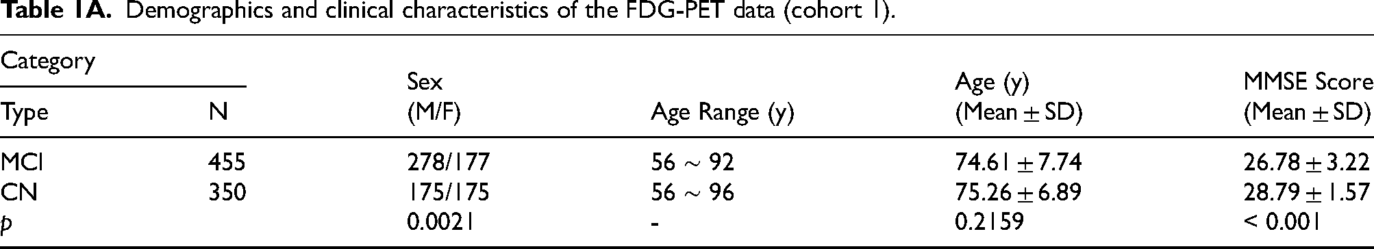
Cohort 1: Individuals underwent an FDG-PET scan (N = 805 participants: n = 350 CN and n = 455 MCI). Table 1A shows demographic information, including age (mean ± standard deviation [SD]), sex, and MMSE scores (mean ± SD).

Table 1A.

Demographics and clinical characteristics of the FDG-PET data (cohort 1).

Category		Sex	Age Range (y)	Age (y)	MMSE Score
Type	N	(M/F)	Age Range (y)	(Mean ± SD)	(Mean ± SD)
MCI	455	278/177	56 ∼ 92	74.61 ± 7.74	26.78 ± 3.22
CN	350	175/175	56 ∼ 96	75.26 ± 6.89	28.79 ± 1.57
p		0.0021	-	0.2159	< 0.001

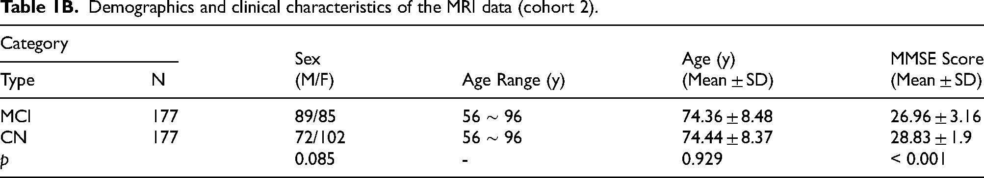
Cohort 2: Individuals underwent brain MRI with T1-weighted and rs-fMRI acquisitions (N = 348 participants: n = 174 CN and n = 174 MCI).

Table 1B shows demographic information for this cohort.

Table 1B.

Demographics and clinical characteristics of the MRI data (cohort 2).

Category		Sex	Age Range (y)	Age (y)	MMSE Score
Type	N	(M/F)	Age Range (y)	(Mean ± SD)	(Mean ± SD)
MCI	177	89/85	56 ∼ 96	74.36 ± 8.48	26.96 ± 3.16
CN	177	72/102	56 ∼ 96	74.44 ± 8.37	28.83 ± 1.9
p		0.085	-	0.929	< 0.001

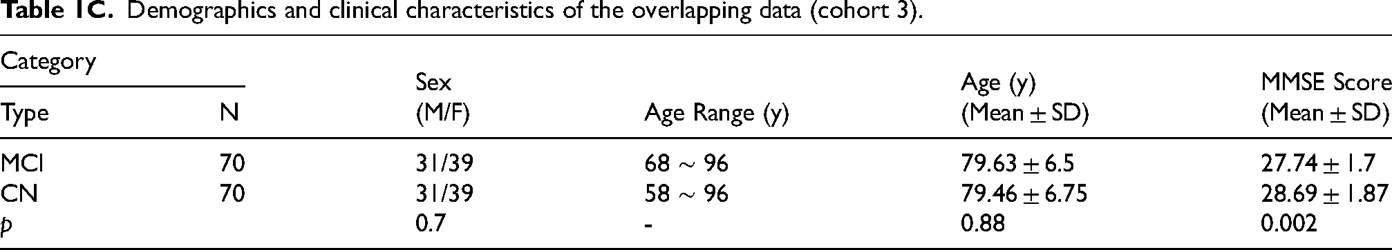
Cohort 3: Individuals that underwent both FDG-PET, T1-weighted MRI, and rs-fMRI acquisitions (N = 140 participants: n = 70 CN and n = 70 MCI).

Table 1C provides the demographic details for cohort 3.

Table 1C.

Demographics and clinical characteristics of the overlapping data (cohort 3).

Category		Sex	Age Range (y)	Age (y)	MMSE Score
Type	N	(M/F)	Age Range (y)	(Mean ± SD)	(Mean ± SD)
MCI	70	31/39	68 ∼ 96	79.63 ± 6.5	27.74 ± 1.7
CN	70	31/39	58 ∼ 96	79.46 ± 6.75	28.69 ± 1.87
p		0.7	-	0.88	0.002

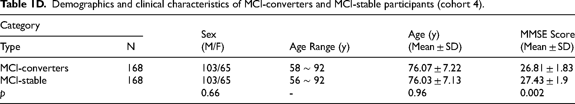
Cohort 4: A subset of individuals from cohort 1 that did or did not convert from MCI to AD dementia (N = 336 participants: n = 168 MCI-converters and n = 168 MCI-stable).

Table 1D shows demographic details, including age, sex, and MMSE scores for cohort 4.

Table 1D.

Demographics and clinical characteristics of MCI-converters and MCI-stable participants (cohort 4).

Category		Sex	Age Range (y)	Age (y)	MMSE Score
Type	N	(M/F)	Age Range (y)	(Mean ± SD)	(Mean ± SD)
MCI-converters	168	103/65	58 ∼ 92	76.07 ± 7.22	26.81 ± 1.83
MCI-stable	168	103/65	56 ∼ 92	76.03 ± 7.13	27.43 ± 1.9
p		0.66	-	0.96	0.002

The inclusion for cohort 1 was the availability of FDG-PET data. The first available FDG-PET was selected, while subsequent sessions were ignored. The inclusion for cohort 2 was the availability of T1-weighted MRI and rs-fMRI. In cohort 2, participants were excluded based on evidence of image artifacts or unusable matrix size for rs-fMRI data (see the CONSORT-style diagram in Figure 1). Participants were excluded if their rs-fMRI data had slice artifacts, high movement peaks, an inconsistent number of volumes (≥976), a matrix size equal to or larger than 88 × 88 × 64, or if the pulse-sequence repetition time (TR) was inconsistent and listed as 0.607 s. Initially, 810 participants were accessed for eligibility. After excluding those with larger matrix sizes, inconsistent pulse-sequence TRs, or inconsistent numbers of volumes (n = 153), 657 participants remained. From this group, 93 participants were excluded due to slice artifacts or high movement peaks. To balance the MCI and CN groups, an additional 216 participants were randomly excluded, resulting in 174 participants each for the MCI and CN groups.

Figure 1.

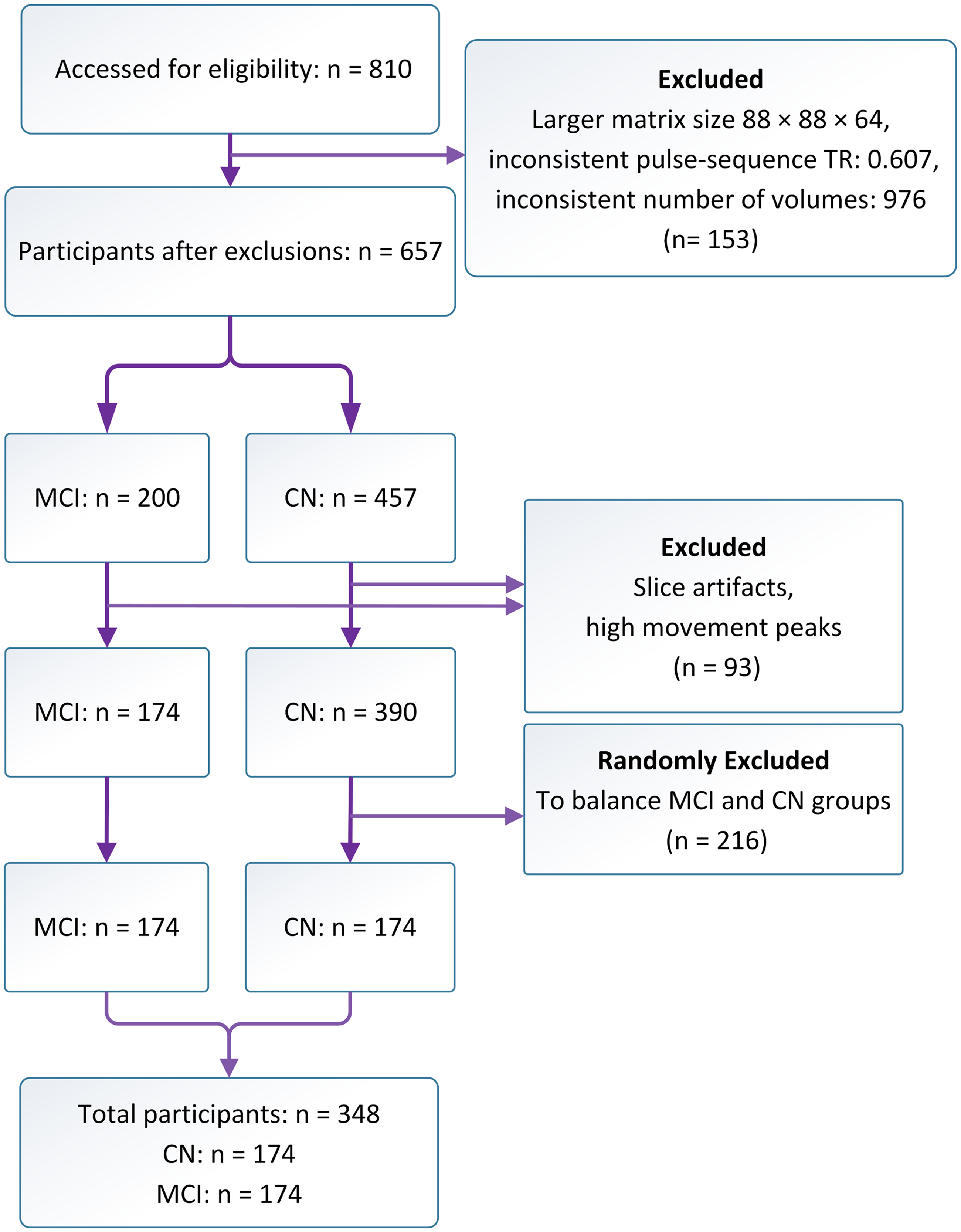
CONSORT-style diagram demonstrating the MRI data quality control process, including screening for exclusion criteria, resulting in the final analyzed MRI sample.

For cohort 4, MCI-converters participants were included based on the availability of FDG-PET data from cohort 1. Cohort 1 had 264 MCI-stable, 168 MCI-converters, and 23 MCI-to-CN subjects. To achieve a balanced cohort 4, the MCI-to-CN individuals were ignored, and a random sample was drawn from the MCI-stable group to match the MCI-converters. Hence, a total of 168 MCI-converters and 168 MCI-stable individuals were used for this cohort.

The ADNI study employs a comprehensive longitudinal follow-up protocol to confirm MCI and CN status. MCI diagnosis was supported by tracking the progression of symptoms over time through repeated clinical evaluations, neuropsychological testing, and imaging studies. Specifically, individuals with MCI were monitored for conversion to AD (MCI-converters) or for stability (MCI-stable). In cohort 4, the time to convert to AD dementia was 60 ± 33 months. Similarly, CN participants were monitored to ensure they do not develop signs of cognitive impairment or dementia during follow-up evaluations (https://adni.loni.usc.edu/study-design).

FDG-PET data preprocessing

FDG-PET were processed using a standardized procedure: images were (1) co-registered to minimize motion effects, (2) averaged to create a single volume from the 30-min PET acquisition, and (3) the baseline PET scan was reoriented into a standardized image grid with 160 × 160 × 96 voxels, each measuring 1.5 mm isotropic. Aligned with the AC-PC line, this grid was the reference image for all subsequent PET scans of the same subject. Co-registration of the frames from each PET scan to the baseline reference image ensures consistent spatial alignment. Additionally, intensity normalization was applied using a subject-specific mask, ensuring uniformity in voxel intensities across scans. (4) Images were smoothed to an isotropic resolution of 8 mm full width at half maximum (FWHM).

The FDG-PET data (160 × 160 × 96 voxels) were downsampled to 64 × 64 × 38 voxels using FLIRT in FSL (FMRIB Software Library).³³ This approach was chosen to improve computational efficiency and create data inputs that would be comparable to the rs-fMRI model (see below). FDG-PET images underwent skull stripping using SynthStrip³⁴ in FreeSurfer.³⁵

rs-fMRI data preprocessing

The rs-fMRI were acquired at 3 Tesla with matrix dimensions of 64 × 64 × 48, an echo time (TE) of 30 ms, and TR of 3 s. Data were acquired using scanners from Siemens, Philips, and GE Medical Systems. rs-fMRI data preprocessing was performed using a combination of FSL and AFNI (Analysis of Functional NeuroImages)³⁶ software packages. The preprocessing pipeline involved: (1) removing the first four volumes, (2) motion correction by aligning the data to the average of the time series, and (3) Skull stripping using FSL's Brain Extraction Tool (BET). ALFF maps were generated using a combination of FSL and AFNI tools: despiking, linear trend removal, and spatial smoothing with a 6 mm FWHM Gaussian kernel. rs-fMRI data were band-pass filtered (0.01–0.08 Hz) and transformed to the frequency domain using the fast Fourier transform. The power spectrum (PS) was calculated, and ALFF was obtained by summing the square root of PS in the low-frequency range (equation 1):

A L F F = s u m (\sqrt{P S (0.01 H z \leq f \leq 0.08 H z)})

(1)

ALFF data were globally intensity normalized and rescaled between 0 and 1.

T1-weighted MRI data preprocessing

T1-weighted MRI were acquired at 3 Tesla with voxel dimensions of 1–1.2 mm × 1 mm × 1 mm, TE/TR = 2.9–3.2/6.5–2.3 ms, and inversion time was 0.4–0.9 ms. T1 images were (1) downsampled to match the voxel dimension of rs-fMRI maps, (2) skull stripped to isolate brain tissues using SynthStrip, and (3) globally intensity normalized and rescaled between 0 and 1.

One-channel DenseNet image-based classifier

We implemented a total of three one-channel 3D DenseNet architectures to classify MCI versus CN individuals, taking advantage of the dense connections for optimizing the volatility of parameters; giving strong regularization; facilitating information flow; and capturing complex spatial patterns inherent in 3D images.³² These networks were trained using FDG-PET, ALFF, or T1-weighted MRI inputs, as illustrated in Figure 2A. MRI models had three dense blocks, each with four layers after the initial layer. The FDG-PET model had four dense blocks comprising 5, 6, 6, and 5 layers, respectively, after the initial layer.

Figure 2.

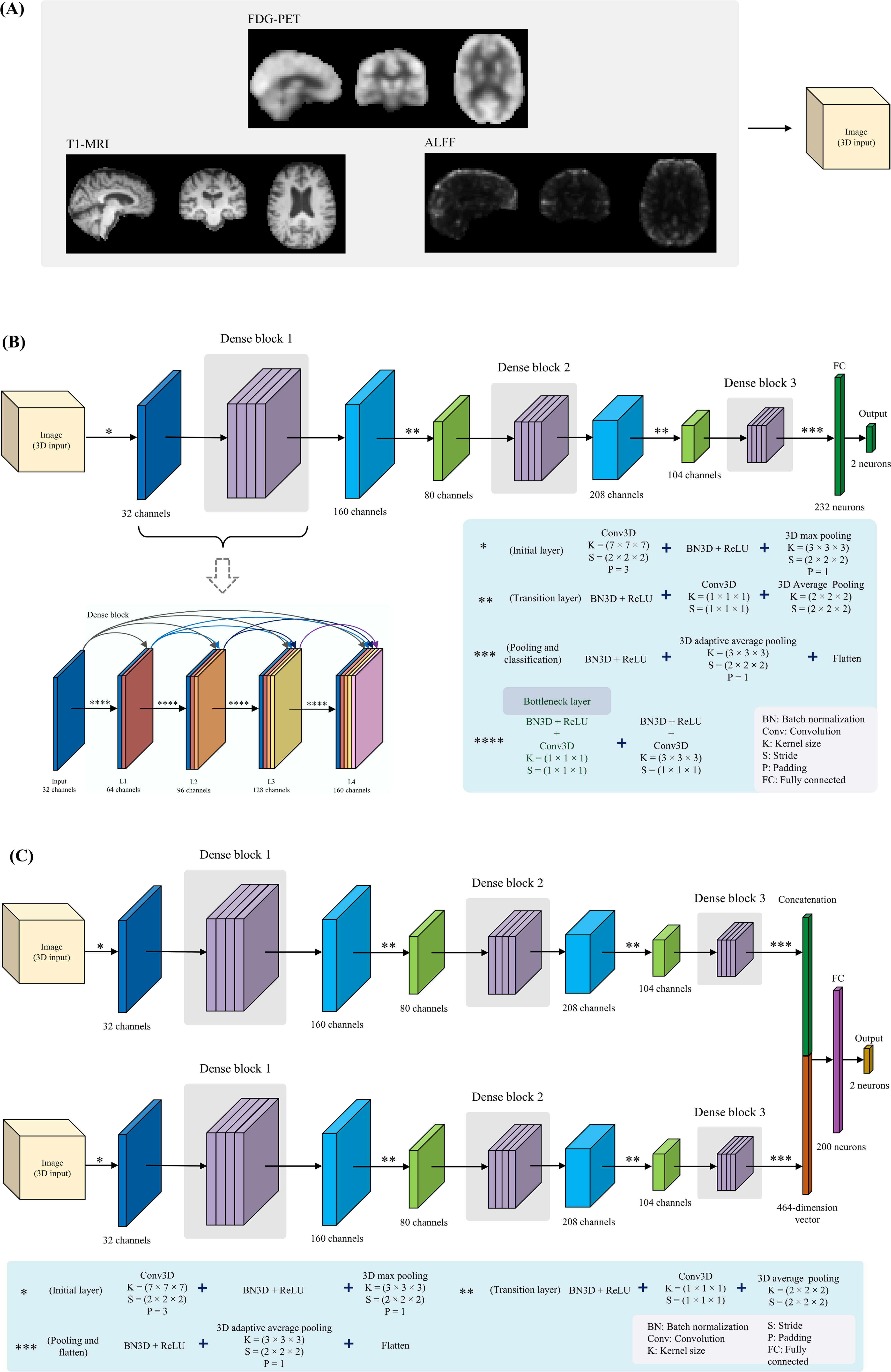
The various image types (ALFF feature map, preprocessed T1-weighted MRI, and FDG-PET) (A), the overall architecture of the proposed 3D one-channel DenseNet model (B), and the proposed 3D two-channel DenseNet model (C).

The 3D DenseNet model contained an initial convolutional layer with 32 filters, a 7 × 7 × 7 kernel size, a stride of 2, and 3D padding of 3. A batch normalization (BN) layer and rectified linear units (ReLU) activation were applied after the convolution (Conv). The feature maps were downsampled using a 3 × 3 × 3 3D max pooling layer with a stride of 2 and padding of 1. The layers in the dense blocks were 3D convolution layers with a growth rate of 32 filters. Also, layers inside each dense block used a bottleneck structure - a 1 × 1 × 1 convolution before each 3 × 3 × 3 convolution - to improve computational efficiency and reduce the input features and the number of parameters while allowing reuse of features across layers via the connectivity pattern.^37,38 BN and ReLU activations were applied after each convolution to enable deep network training. Each layer within a dense block performs a non-linear transformation, denoted by $H_{l} (.)$ , where l indicates the layer's position. $H_{l} (.)$ combines bottleneck layer operations with a 3 × 3 × 3 convolution. The bottleneck layer (with size 4) reduces output channels to $4 k$ , where k is the growth rate. It includes (1) BN, (2) ReLU, and (3) 1 × 1 × 1 Conv. Each subsequent layer performs (1) BN, (2) ReLU, and (3) a 3 × 3 × 3 Conv. The input feature maps to layer l equal $k_{0} + k \times (l - 1)$ , where $k_{0}$ is the initial number of channels and k the growth rate. In our models trained on MRI data, with four layers per dense block ( $l$ = 1 to 4) and a growth rate of 32, each layer produces 32 new feature maps. DenseNet connections concatenate these outputs and provide subsequent layers with collective knowledge from earlier ones and enabling the extraction of higher-level information.

Transition layers between dense blocks downsample feature maps by performing (1) BN, (2) ReLU, (3) 1 × 1 × 1 3D convolution, and (4) average pooling (2 × 2 × 2 kernel, stride 2).

After the final dense block, the network aggregated and classified features using: (1) BN, (2) ReLU, (3) Adaptive average pooling (reducing 3D feature maps to 1D vectors), (4) Flatten (concatenating pooled vectors), (5) an FC layer for high-level feature learning, and (6) an output FC linear layer with two neurons.

The training loss was computed by comparing the neuron outputs with the ground truth labels using a Cross-Entropy loss function from PyTorch (version 2.0.0),³⁹ which applies to log SoftMax internally and calculates negative log-likelihood. The 3D DenseNet model architecture trained on MRI data is illustrated in Figure 2B, showing the overall structure with the initial layer, dense blocks, transition layers, and final layers.

Two-channel DenseNet image-based classifier

One 3D two-channel DenseNet model was trained and relied on ALFF and T1 inputs. The architecture of each channel is identical to the 3D one-channel DenseNet designed for MRI data. A key difference was the final FC layer. After flattening the outputs of the adaptive average pooling layer from each channel, the features were concatenated, resulting in a combined feature vector of 464 (2 × 232 from each channel). This joint feature vector concatenating information from both channels was passed through an FC layer with 200 neurons, followed by the final 2-neuron classification output layer.

Figure 2C illustrates the model structure, emphasizing the dense connectivity layers processing each volume and the joint FC layers for classification. The training methodology aligned with the one-channel model and facilitated specialized learning on different data types.

Model evaluation and training strategies

The one-channel MRI models had 1.56 million trainable parameters, while the FDG-PET model had 3.1 million. For cohort 3, the overlapping sample between cohorts 1 and 2, we used the same architecture with 1.56 million trainable parameters for all data types (FDG-PET, T1-weighted, and ALFF). The two-channel models contained over 3.22 million trainable parameters. For cohort 3, we trained two-channel models on every paired combination of data types. We conducted one additional experiment where a one-channel model was trained using T1-weighted MRI images closer to the original spatial resolution. For cohort 4, we used a one-channel FDG-PET model, identical to the one for cohort 3, with 1.56 million trainable parameters, to predict MCI-converters.

Model evaluation was based on a 10% hold-out test set and a 10-fold cross-validation (CV) on the remaining 90% of the data.

Class weights, calculated based on training data class frequencies, were applied to the loss function of the FDG-PET-based model to address class imbalance. Adam⁴⁰ was used to update model weights adaptively based on stochastic gradients. A small weight decay of 0.0001 was applied as regularization to prevent overfitting. The schedule allows using a larger learning rate initially for faster convergence, then decreasing it for fine-tuning. All models were trained for 250 epochs with a batch size of 8. A dropout rate of 0.1 was used for regularization. The initial learning rate was set to 0.00002 and reduced by half at epochs 30 and 120 using the scheduler. Random rotations of up to π/6 radians and zooms from 0.9× to 1.1× were applied with 50% probability per sample for data augmentation. This data augmentation provided variations in orientation and scale to improve generalization.

3D DenseNet one channel models were trained for 13 to 28 h and the two-channel ALFF-T1 model required 16 h of training. The models aligned with tools from the MONAI library (version 1.2.dev2305)⁴¹ in Python 3.10 (python.org) and were trained on four NVIDIA V100 GPUs (32GB of HBM2 memory) from the Digital Research Alliance of Canada (alliancecan.ca).

Statistical analysis

Statistical analysis was performed using Python 3.10 with the SciPy library (version 1.8.1)⁴² to test for group differences in demographic and clinical characteristics. The demographic variables were summarized using descriptive statistics. Sex was presented as frequency counts for the MCI and CN groups to represent their distribution. Continuous variables, including age and MMSE scores, were reported as mean ± SD for both groups. An independent sample t-test was used to compare the mean age and MMSE scores between the MCI and CN groups. A chi-square test was used to compare the sex distribution. Classification metrics were generated through 10-fold of cross-validation for all four of the models that were trained (i.e., FDG-PET, ALFF, T1, ALFF-T1), which allowed for hypothesis testing. Classification performance was evaluated through receiver operator characteristics (ROC) analysis. A one-way analysis of variance (ANOVA) was conducted to compare the accuracy, sensitivity, and specificity results. Post-hoc corrected paired t-tests were performed to directly compare model accuracy results.

Results

Demographic differences: MCI versus CN

The demographic characteristics of study participants are shown in Table 1A (FDG-PET) and Table 1B (MRI). The two groups from cohort 1 were matched for age (p = 0.2159) but not sex (p = 0.0021) and had different MMSE scores (as expected, p < 0.001). The two groups from cohort 2 were matched for age and sex (p > 0.08) and had different MMSE scores (p < 0.001). For the overlapping data in cohort 3, as detailed in Table 1C, the MCI and CN groups were matched for sex (p = 0.7) and age (p = 0.88), and had different MMSE scores (p = 0.002). In cohort 4, the groups (MCI-converters and MCI-stable) were matched for age (p = 0.96) and sex (p = 0.66), but showed significant differences in MMSE scores (p = 0.002), as presented in Table 1D.

Comparing model performance

In cohorts 1 and 2, the highest classification accuracy was 88.02% ± 3.82, corresponding to the FDG-PET model. The accuracy results showed a significant model effect (F(3, 36) = 54.85, p < 0.001). Similarly, there was a significant model effect for the sensitivity metric (F(3, 36) = 9.18, p < 0.001). And this was the case for specificity (F(3, 36) = 43.53, p < 0.001).

Corrected paired t-tests (Table 2) revealed that the FDG-PET model had higher accuracy than all three of the MRI models (p < 0.001) for cohorts 1 and 2. The ALFF-T1 model had higher accuracy than the T1 model (p < 0.001). The ALFF model had higher accuracy than the T1 model (p < 0.001).

Table 2.

Pairwise comparison of group means and corrected paired t-test results. A positive t-statistic indicates greater accuracy for the model listed in the ‘Data type 1’ column.

Comparison		Cohorts	t-statistic	p
Data type 1	Data type 2	Cohorts	t-statistic	p
FDG-PET	T1	1, 2	11.1	<0.001
FDG-PET	ALFF	1, 2	3.8	0.004
FDG-PET	ALFF, T1	1, 2	5.26	<0.001
T1	ALFF, T1	2	−11.1	<0.001
ALFF	T1	2	5.16	<0.001
ALFF	ALFF, T1	2	−1.71	0.12
FDG-PET	T1	3	2.07	0.068
FDG-PET	ALFF	3	1.78	0.1
FDG-PET	ALFF, T1	3	0.78	0.45
FDG-PET	FDG-PET, T1	3	−0.53	0.6
FDG-PET	FDG-PET, ALFF	3	−0.56	0.59
T1	ALFF	3	−0.73	0.48
T1	ALFF, T1	3	−1.48	0.17
T1	FDG-PET, T1	3	−3.31	0.009
T1	FDG-PET, ALFF	3	−3.06	0.013
ALFF	ALFF, T1	3	−0.77	0.46
ALFF	FDG-PET, T1	3	−2.54	0.03
ALFF	FDG-PET, ALFF	3	−2.69	0.025
FDG-PET, T1	ALFF, T1	3	1.19	0.26
FDG-PET, T1	FDG-PET, ALFF	3	−0.42	0.68
FDG-PET, ALFF	ALFF, T1	3	1.72	0.12

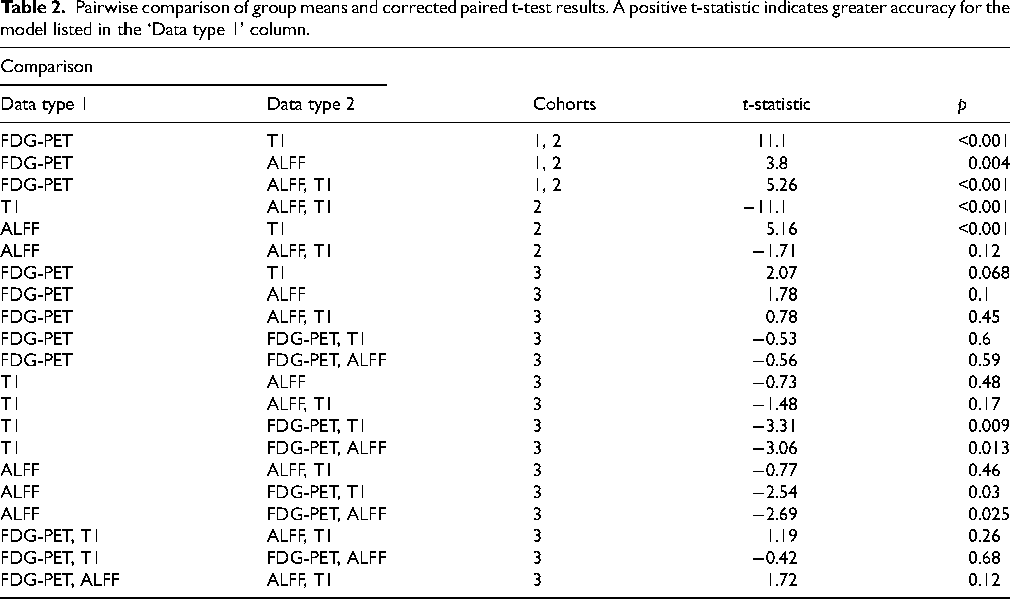
In cohort 3, there was a significant accuracy difference between the models (F(5, 54) = 3.32, p = 0.01); namely, the two-channel model using FDG-PET and T1 data achieved an accuracy of 71.43% ± 10.5, which was higher than the T1 one-channel model (t = 3.31, p = 0.009). The two-channel model with FDG-PET and ALFF inputs performed better than the individual ALFF one-channel model (t = 2.69, p = 0.025). Table 2 includes all corrected paired t-test results.

The classification performance did not improve for the higher resolution T1-weighted MRI inputs, achieving an overall accuracy of 52.86% ± 3.15, compared to 54% ± 3.49 with the lower resolution inputs (t = 0.475, p = 0.65).

In cohort 4, the one-channel FDG-PET model achieved an accuracy of 63.23% ± 4.68 in predicting MCI-converters relative to MCI-stable, with sensitivity of 64.71% ± 8.87, and specificity of 61.77% ± 7.75.

Figure 3A displays the average confusion matrix for the FDG-PET model across the 10 cross-validation folds to classify MCI versus CN. Figure 3B shows ROC curves for the FDG-PET model with corresponding AUC values for each fold. Furthermore, Figure 3C presents a comparison of metrics among different models (FDG-PET, ALFF-T1, ALFF, and T1).

Figure 3.

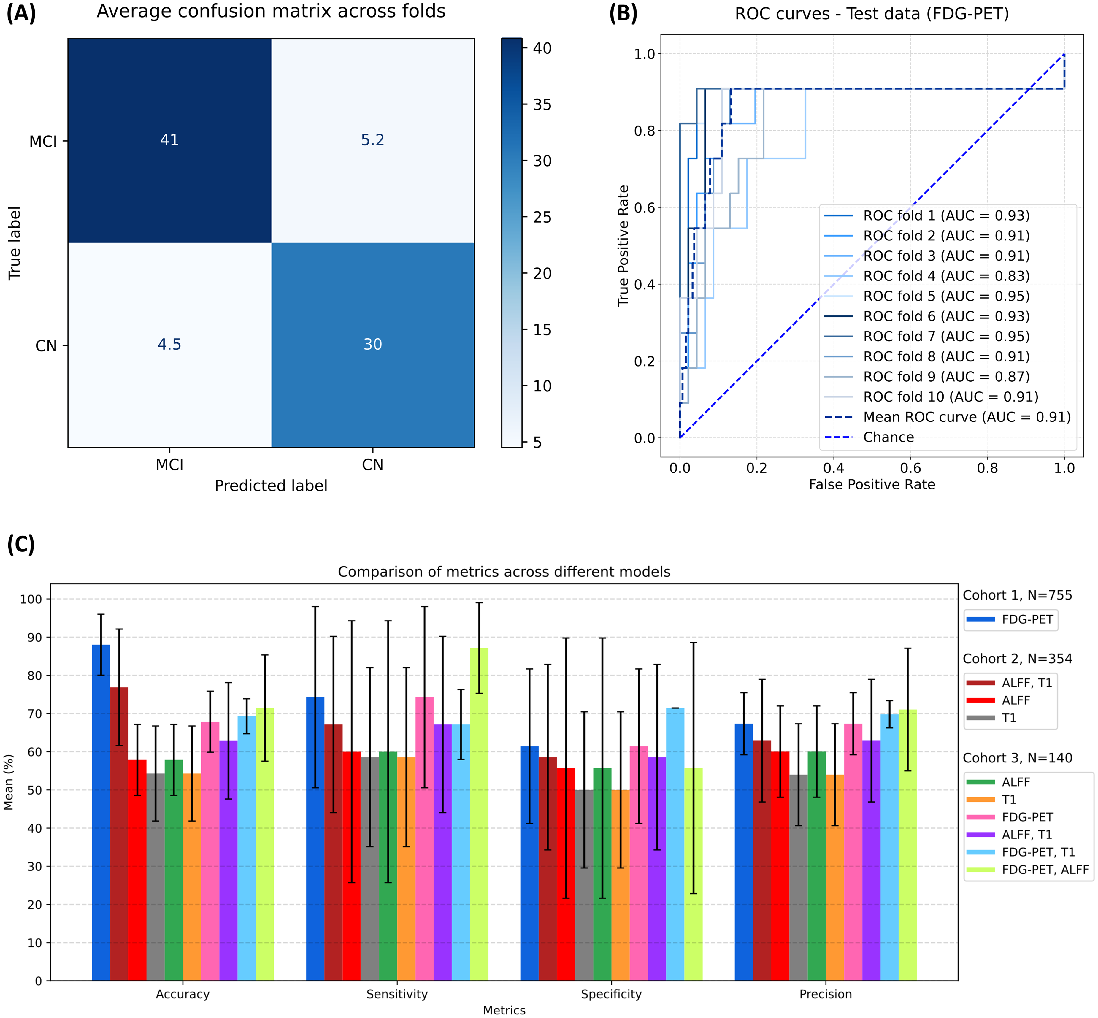
The results of classification models: (A) The FDG-PET confusion matrix results are the average over 10 cross-validation folds to classify MCI versus CN, hence non-integer values. (B) ROC curves and associated AUC metrics of the FDG-PET model on the test data to classify MCI versus CN. (C) Metric comparisons among different models.

Discussion

The current study demonstrates that whole brain neuroimaging data can be used to perform automated classification of MCI compared to CN individuals in a deep learning 3D DenseNet framework. Contrary to our hypothesis, we found that the one-channel FDG-PET model achieved higher classification accuracy, sensitivity, and specificity than the two-channel ALFF-T1 model. The one-channel ALFF model had the next highest performance, followed by the T1 model which had low accuracy and specificity. Lastly, it was possible to achieve better-than-chance accuracy in predicting future MCI-converters based on the FDG-PET. Collectively, the findings are novel and demonstrate that 3D images can be used in isolation or stacked into a two-channel model to perform MCI classification tasks.

The one-channel FDG-PET model had the highest accuracy, sensitivity, and specificity relative to the three other models. The superiority of the FDG-PET to classify MCI versus CN reflects the following possible influences. Several studies have demonstrated increased glucose utilization in the entorhinal cortex, hippocampus, and frontal cortex regions⁴³ and reduced glucose in temporal, parietal, and occipital lobes for MCI relative to CN.⁴⁴ These sources of spatial variation in brain metabolism in MCI is one reason why the FDG-PET model achieved higher classification performance. Hypometabolism detected by FDG-PET tends to precede brain volume loss, providing an early marker of neurodegenerative changes. This is supported by FDG-PET studies in presymptomatic familial AD patients, which showed widespread reductions in cerebral metabolic rate for glucose in brain regions typically affected in AD, including the medial temporal lobe, well before significant volume loss occurred.⁴⁵ It should be noted that FDG-PET hypometabolism in MCI can be influenced directly from amyloid and tau AD pathologies.^46–48 As demonstrated by Mattsson-Carlgren et al. (2020), Aβ deposition is associated with increases in soluble and phosphorylated tau that precede a positive tau PET in AD. This temporal relationship underscores the early detection capabilities of FDG-PET.⁴⁹ It is notable that the ALFF-T1 model, which reflects the combined influenced of neurovascular physiology and anatomy, had the next best performance metrics.

The MRI-based DenseNet models were inferior to FDG-PET but there are important findings to discuss. The ALFF-T1 MRI model had reasonably high-performance metrics, which lends credence to clinical MRI protocols that capture non-invasive measures of brain function and anatomy. The ALFF-T1 results suggest MRI data could be used for staging MCI. Although beyond the scope of the current study, MRI-based classification metrics could be used alongside cognitive and other clinical variables to produce an MCI risk profile. The MRI data were collected across multiple sites and scanners and therefore it was deemed prudent to incorporate widely accepted processing steps for these data prior to model training. The ALFF-T1 and ALFF models were clearly better than the T1 model results, which is interesting given the number of machine learning findings that report high classification accuracy using exclusively anatomical data.^50–52 There are several reasons to explain the low classification accuracy for the T1 models. The T1 data were downsampled to be comparable to FDG-PET and ALFF images. This study design choice likely contributed to classification performance hence the T1 model results should be viewed with some caution. Future work could include variable image resolutions for data inputs, but this complicates the model framework and was beyond the scope of this 3D DenseNet feasibility study.

The ANOVA results revealed significant differences in sensitivity and specificity across the models, with the FDG-PET model exhibiting the highest values for both metrics (sensitivity: 88.70% ± 4.70, specificity: 87.14% ± 5.03). The FDG-PET model's high sensitivity suggests a low risk of overlooking individuals with MCI, as early intervention is key in managing cognitive decline. Additionally, the model's high specificity indicates a low rate of false positives, which reduces unnecessary follow-up tests and interventions for those who do not have MCI, thus saving resources and minimizing patient anxiety.

We performed additional analysis based on the overlapping data from cohorts 1 and 2. These results could be viewed as more exploratory given the smaller sample size for cohort 3, however, the findings were insightful. Combining FDG-PET with each of the MRI data sources in respective two-channel models improved classification compared to using T1-weighted MRI or ALFF alone. Although the two-channel model combining FDG-PET and T1-weighted MRI had the highest accuracy, it was not significantly better than the FDG-PET alone model. More work is needed to help clarify which combination of image sources can yield even higher classification results.

The use of deep learning in AD is evolving rapidly, hence the opportunity to position the current study in the literature. Liu et al.⁵³ used deep learning and machine learning techniques such as 2D CNNs and recurrent neural networks like bidirectional gated recurrent units, and Li et al.⁵⁴ employed principal component analysis on PET, MRI, and cerebrospinal fluid, combined with the MMSE and Alzheimer's Disease Assessment Scale-Cognitive subscale, to train a deep neural network framework with restricted Boltzmann machine. In contrast, our study solely used FDG-PET with a modified 3D deep learning architecture, specifically a one-channel 3D-DensNet model, which resulted in higher accuracy in diagnosing MCI. Additionally, Suk et al.⁵⁵ used rs-fMRI data with a deep auto-encoder for MCI diagnosis. Still, our two-channel DenseNet model outperformed using a single modality, incorporating both rs-fMRI and T1-MRI.

The current study has some limitations that are discussed herein. We did not consider an AD sample because the goal was to focus on MCI versus CN classification and provide potential automated decision support during the earlier stages of AD. We note that cohort 1 (FDG-PET) had a larger sample size compared to cohort 2. There are several directions to pursue for 3D DenseNet classification models, notably use of diffusion tensor imaging that Rallabandi et al.⁵⁶ exploited in a random forest framework to perform MCI versus CN classification. In principle, it is feasible to add more channels to a stacked DenseNet. Next, we did not include amyloid nor tau PET images, despite their diagnostic relevance. When accessing ADNI data we noted the sample sizes for these PET data were smaller than FDG-PET. Naturally, it would be important to consider these data sources as part of a comprehensive and automated AD imaging framework. Similarly, for MRI data, T2-weighted images can be used to accentuate temporal lobe imaging features, as demonstrated by Liu et al.⁵⁷ in their 3D-CNN. The FDG-PET model had one more dense block compared to MRI models. This decision was made because we only considered a one-channel FDG-PET model in cohort 1. The extra dense block results in a similar number of trainable parameters relative to the ALFF-T1 model, which helps in interpreting the results from these different models. It is not possible to comment on the role of partial volume effects for any of the four models; however, we attempted to match the image inputs prior to model training. Higher resolution T1-weighted MRI inputs did not improve performance. Thus, we used low-resolution inputs to ensure uniformity across all images, avoiding biases from varying resolutions, and reducing memory and processing time requirements. Ideally, full and/or higher-resolution image inputs are desirable but beyond the scope of the current study.

The use of FDG-PET data resulted in better-than-chance accuracy in predicting individuals that would convert to AD dementia in the future; however, the performance metrics reveal there is still room for improvement. These findings reflect the inherent complexity of this clinical challenge, where subtle and overlapping biomarkers complicate accurate classification.⁵⁸ The moderate predictive capability suggests that while the model captures relevant patterns, it may be limited by the heterogeneity of the MCI population and the between-subject differences in disease progression.⁵⁹ Long-term prediction accuracy is often limited by the unpredictability of intermediate disease stages, which can show fluctuating biomarker levels.⁶⁰ Enhancing predictive power may require integrating multimodal imaging data (e.g., amyloid PET, tau PET) or non-imaging biomarkers like plasma p-tau217 and p-tau181, which has shown strong associations with MCI conversion.^61,62 In the context of a 60-month prediction horizon, the FDG-PET model's performance can be considered robust, yet further refinement, particularly through the integration of additional longitudinal data, could better capture the temporal dynamics of cognitive decline. This would potentially improve the model's ability to generalize across diverse patient profiles and make it more robust for real-world applications.

Conclusion

The application of neuroimaging methods has provided new insights into MCI diagnosis. The FDG-PET model's individual training performance indicates that it has a distinct ability to classify MCI versus CN. Training a two-channel model with both T1-weighted MRI and rs-fMRI data led to superior diagnostic performance compared to models relying on a single MRI modality. While this result supports the power of the two-channel (ALFF-T1) approach for MCI diagnosis, it reveals that the FDG-PET model individually surpassed the two-channel MRI-based model. Although MRI-based automated estimates did not surpass the accuracy of FDG-PET, our results demonstrate the value of using multi-contrast MRI for image-based classification of neurodegeneration. This study highlights the potential of advanced deep-learning approaches to improve early detection and intervention for those at risk of major neurocognitive disorders.

Footnotes

Acknowledgments

BJM acknowledges support from the Sandra Black Centre for Brain Resilience and Recovery. This research was enabled in part by support provided by the Digital Research Alliance of Canada (alliancecan.ca).

ORCID iDs

Iman Jahani

Ali Jahani

Mehdi Delrobaei

Ali Khadem

Bradley J. MacIntosh

Author contributions

Iman Jahani (Conceptualization; Formal analysis; Methodology; Software; Validation; Visualization; Writing – original draft; Writing – review & editing); Ali Jahani (Conceptualization; Formal analysis; Methodology; Software; Validation; Visualization; Writing – original draft; Writing – review & editing); Mehdi Delrobaei (Conceptualization; Supervision; Validation; Writing – review & editing); Ali Khadem (Conceptualization; Supervision; Validation; Writing – review & editing); Bradley J MacIntosh (Conceptualization; Formal analysis; Funding acquisition; Methodology; Project administration; Supervision; Validation; Writing – original draft; Writing – review & editing).

Funding

The authors disclosed receipt of the following financial support for the research, authorship, and/or publication of this article: We acknowledge grant funding provided to BJM from the Canadian Institutes of Health Research (PJT-165981).

Declaration of conflicting interests

The authors declared no potential conflicts of interest with respect to the research, authorship, and/or publication of this article.

Data availability

The data supporting the findings of this study are openly available in ADNI at https://adni.loni.usc.edu/data-samples/access-data/. These data were derived from the following resources available in the public domain: .

References

Jack

Jr. Andrews

Beach

, et al. Revised criteria for diagnosis and staging of Alzheimer's disease: alzheimer's Association Workgroup. Alzheimers Dement 2024; 20: 5143–5169.

Bertens

Vos

Kehoe

, et al. Use of mild cognitive impairment and prodromal AD/MCI due to AD in clinical care: a European survey. Alzheimers Res Ther 2019; 11: 74.

Jack

Jr. Bennett

Blennow

, et al. NIA-AA Research Framework: toward a biological definition of Alzheimer's disease. Alzheimers Dement 2018; 14: 535–562.

Rajan

Weuve

Barnes

, et al. Population estimate of people with clinical Alzheimer's disease and mild cognitive impairment in the United States (2020–2060). Alzheimers Dement 2021; 17: 1966–1975.

Shigemizu

Akiyama

Higaki

, et al. Prognosis prediction model for conversion from mild cognitive impairment to Alzheimer's disease created by integrative analysis of multi-omics data. Alzheimers Res Ther 2020; 12: 145.

Nettiksimmons

DeCarli

Landau

, et al. Biological heterogeneity in ADNI amnestic mild cognitive impairment. Alzheimers Dement 2014; 10: 511–521 e511.

Arevalo-Rodriguez

Smailagic

Roque-Figuls

, et al. Mini-Mental State Examination (MMSE) for the early detection of dementia in people with mild cognitive impairment (MCI). Cochrane Database Syst Rev 2021; 7: CD010783.

Matallana

de Santacruz

Cano

, et al. The relationship between education level and mini-mental state examination domains among older Mexican Americans. J Geriatr Psychiatry Neurol 2011; 24: 9–18.

Ries

Carlsson

Rowley

, et al. Magnetic resonance imaging characterization of brain structure and function in mild cognitive impairment: a review. J Am Geriatr Soc 2008; 56: 920–934.

10.

Zeng

Luo

, et al. Decoupling of regional cerebral blood flow and brain function along the Alzheimer's disease continuum. J Alzheimers Dis 2023; 95: 287–298.

11.

Bollack

Pemberton

Collij

, et al. Longitudinal amyloid and tau PET imaging in Alzheimer's disease: a systematic review of methodologies and factors affecting quantification. Alzheimers Dement 2023; 19: 5232–5252.

12.

Shimohama

Tezuka

Takahata

, et al. Impact of amyloid and tau PET on changes in diagnosis and patient management. Neurology 2023; 100: e264–e274.

13.

Lee

Youn

Jeong

, et al. Cost-effectiveness of using amyloid positron emission tomography in individuals with mild cognitive impairment. Cost Eff Resour Alloc 2021; 19: 50.

14.

Jie

Treyer

Schibli

, et al. Tauvid: the first FDA-approved PET tracer for imaging tau pathology in Alzheimer's disease. Pharmaceuticals (Basel) 2021; 14: 110.

15.

Calandrelli

Panfili

Onofrj

, et al. Brain atrophy pattern in patients with mild cognitive impairment: MRI study. Transl Neurosci 2022; 13: 335–348.

16.

Ibrahim

Suppiah

Ibrahim

, et al. Diagnostic power of resting-state fMRI for detection of network connectivity in Alzheimer's disease and mild cognitive impairment: a systematic review. Hum Brain Mapp 2021; 42: 2941–2968.

17.

Palesi

Castellazzi

Casiraghi

, et al. Exploring patterns of alteration in Alzheimer's disease brain networks: a combined structural and functional connectomics analysis. Front Neurosci 2016; 10: 80.

18.

Lama

Kwon

. Resting-state functional connectivity difference in Alzheimer's disease and mild cognitive impairment using threshold-free cluster enhancement. Diagnostics (Basel) 2023; 13: 3074.

19.

Driscoll

Davatzikos

, et al. Longitudinal pattern of regional brain volume change differentiates normal aging from MCI. Neurology 2009; 72: 1906–1913.

20.

Teipel

Wohlert

Metzger

, et al. Multicenter stability of resting state fMRI in the detection of Alzheimer's disease and amnestic MCI. Neuroimage Clin 2017; 14: 183–194.

21.

Ouyang

Yuan

. Deep learning aided neuroimaging and brain regulation. Sensors (Basel) 2023; 23: 4993.

22.

Liu

Masurkar

Rusinek

, et al. Generalizable deep learning model for early Alzheimer’s disease detection from structural MRIs. Sci Rep 2022; 12: 17106.

23.

Wang

Lim

. Zoom-in neural network deep-learning model for Alzheimer's disease assessments. Sensors (Basel) 2022; 22: 8887.

24.

Singh

Srivastava

, et al. Deep learning based classification of FDG-PET data for Alzheimers disease categories. Proc SPIE Int Soc Opt Eng 2017; 10572: 105720J.

25.

Odusami

Maskeliunas

Damasevicius

. Pareto optimized adaptive learning with transposed convolution for image fusion Alzheimer's disease classification. Brain Sci 2023; 13: 1045.

26.

Etminani

Soliman

Davidsson

, et al. A 3D deep learning model to predict the diagnosis of dementia with Lewy bodies, Alzheimer's disease, and mild cognitive impairment using brain 18F-FDG PET. Eur J Nucl Med Mol Imaging 2022; 49: 563–584.

27.

Rogeau

Hives

Bordier

, et al. A 3D convolutional neural network to classify subjects as Alzheimer's disease, frontotemporal dementia or healthy controls using brain 18F-FDG PET. Neuroimage 2024; 288: 120530.

28.

Cao

Nayak

, et al. Deep learning combining FDG-PET and neurocognitive data accurately predicts MCI conversion to Alzheimer's dementia 3-year post MCI diagnosis. Neurobiol Dis 2023; 187: 106310.

29.

Jack

Jr. Knopman

Jagust

, et al. Tracking pathophysiological processes in Alzheimer's disease: an updated hypothetical model of dynamic biomarkers. Lancet Neurol 2013; 12: 207–216.

30.

Zang

Zhu

, et al. Altered baseline brain activity in children with ADHD revealed by resting-state functional MRI. Brain Dev 2007; 29: 83–91.

31.

Deng

Franklin

O'Boyle

, et al. Hemodynamic and metabolic correspondence of resting-state voxel-based physiological metrics in healthy adults. Neuroimage 2022; 250: 118923.

32.

Huang

Liu

van der Maaten

, et al.

Densely connected convolutional networks.

arXiv Prepr 2016: arXiv:1608.06993.

33.

Smith

Jenkinson

Woolrich

, et al. Advances in functional and structural MR image analysis and implementation as FSL. Neuroimage 2004; 23: S208–S219.

34.

Hoopes

Mora

Dalca

, et al. Synthstrip: skull-stripping for any brain image. NeuroImage 2022; 260: 119474.

35.

Fischl

. Freesurfer. Neuroimage 2012; 62: 774–781.

36.

Cox

. AFNI: software for analysis and visualization of functional magnetic resonance neuroimages. Comput Biomed Res 1996; 29: 162–173.

37.

Zhang

Ren

, et al. Deep residual learning for image recognition. In: Proc IEEE Comput Soc Conf Comput Vis Pattern Recognit 27–30 June 2016, pp.770–778.

38.

Szegedy

Vanhoucke

Ioffe

, et al. Rethinking the inception architecture for computer vision. arXiv Prepr 2015: arXiv:1512.00567.

39.

Paszke

Gross

Massa

, et al. Pytorch: an imperative style, high-performance deep learning library. In: Wallach

Larochelle

Beygelzimer

, et al. (eds) Advances in neural information processing systems (NeurIPS 2019). San Diego, CA: Neural Information Processing Systems Foundation Inc, 2020, pp.7994–8005.

40.

Kingma

. Adam: A method for stochastic optimization. arXiv Prepr 2014: arXiv:1412.6980.

41.

Cardoso

Brown

, et al. MONAI: An open-source framework for deep learning in healthcare. arXiv Prepr 2022: arXiv:2211.02701.

42.

Virtanen

Gommers

Oliphant

, et al. Scipy 1.0: fundamental algorithms for scientific computing in python. Nat Methods 2020; 17: 261–272.

43.

Men

Zhu

, et al. Age- and brain region-specific changes of glucose metabolic disorder, learning, and memory dysfunction in early Alzheimer's disease assessed in APP/PS1 transgenic mice using (18)F-FDG-PET. Int J Mol Sci 2016; 17: 1707.

44.

Sanabria-Diaz

Martinez-Montes

Melie-Garcia

, et al. Glucose metabolism during resting state reveals abnormal brain networks organization in the Alzheimer's disease and mild cognitive impairment. PLoS One 2013; 8: e68860.

45.

Mosconi

Pupi

De Leon

. Brain glucose hypometabolism and oxidative stress in preclinical Alzheimer's disease. Ann N Y Acad Sci 2008; 1147: 180–195.

46.

Bischof

Jessen

Fliessbach

, et al. Impact of tau and amyloid burden on glucose metabolism in Alzheimer's disease. Ann Clin Transl Neurol 2016; 3: 934–939.

47.

Maschio

. Amyloid and tau positron emission tomography imaging in Alzheimer's disease and other tauopathies. Front Aging Neurosci 2022; 14: 838034.

48.

Rubinski

Franzmeier

Neitzel

, et al. FDG-PET hypermetabolism is associated with higher tau-PET in mild cognitive impairment at low amyloid-PET levels. Alzheimers Res Ther 2020; 12: 133.

49.

Mattsson-Carlgren

Andersson

Janelidze

, et al. Abeta deposition is associated with increases in soluble and phosphorylated tau that precede a positive Tau PET in Alzheimer's disease. Sci Adv 2020; 6: eaaz2387.

50.

Khan

Kaushik

Chowdhary

, et al. Ensemble model for diagnostic classification of Alzheimer's disease based on brain anatomical magnetic resonance imaging. Diagnostics (Basel) 2022; 12: 3193.

51.

Salvatore

Cerasa

Battista

, et al. Magnetic resonance imaging biomarkers for the early diagnosis of Alzheimer's disease: a machine learning approach. Front Neurosci 2015; 9: 07.

52.

Nanni

Interlenghi

Brahnam

, et al. Comparison of transfer learning and conventional machine learning applied to structural brain MRI for the early diagnosis and prognosis of Alzheimer's disease. Front Neurol 2020; 11: 576194.

53.

Liu

Cheng

Yan

, et al. Classification of Alzheimer's disease by combination of convolutional and recurrent neural networks using FDG-PET images. Front Neuroinform 2018; 12: 35.

54.

Tran

Thung

, et al. A robust deep model for improved classification of AD/MCI patients. IEEE J Biomed Health Inform 2015; 19: 1610–1616.

55.

Suk

Wee

Lee

, et al. State-space model with deep learning for functional dynamics estimation in resting-state fMRI. Neuroimage 2016; 129: 292–307.

56.

Subramanyam Rallabandi

Seetharaman

. Classification of cognitively normal controls, mild cognitive impairment and Alzheimer’s disease using transfer learning approach. Biomed Signal Process Control 2023; 79: 104092.

57.

Liu

Yan

, et al. A multi-model deep convolutional neural network for automatic hippocampus segmentation and classification in Alzheimer's disease. Neuroimage 2020; 208: 116459.

58.

DeMarshall

Nagele

Sarkar

, et al. Detection of Alzheimer's disease at mild cognitive impairment and disease progression using autoantibodies as blood-based biomarkers. Alzheimers Dement (Amst) 2016; 3: 51–62.

59.

Verdi

Kia

Yong

KXX

, et al. Revealing individual neuroanatomical heterogeneity in Alzheimer disease using neuroanatomical normative modeling. Neurology 2023; 100: e2442–e2453.

60.

Maheux

Koval

Ortholand

, et al. Forecasting individual progression trajectories in Alzheimer's disease. Nat Commun 2023; 14: 761.

61.

Mundada

Rojas

Vandevrede

, et al. Head-to-head comparison between plasma p-tau217 and flortaucipir-PET in amyloid-positive patients with cognitive impairment. Alzheimers Res Ther 2023; 15: 157.

62.

Jack

Jr. Wiste

Algeciras-Schimnich

, et al. Comparison of plasma biomarkers and amyloid PET for predicting memory decline in cognitively unimpaired individuals. Alzheimers Dement 2024; 20: 2143–2154.