Determinants of Personal Exposure to PM 2.5 in Office Workers

Abstract

To determine the distribution of personal exposure to PM_2.5 concentrations in office workers and to identify the most important determinants of personal exposure to PM_2.5 concentrations, a couple of 24-h personal exposures and indoor home and office PM_2.5 concentrations were measured among 40 non-smoker adult subjects over a year. All subjects completed a Time-Microenvironment-Activity–Dairy (TMAD) and a core questionnaire that covered air quality-related characteristics of each subject microenvironments and some personal characteristics that related to personal exposure to particulate matter. Participant’s exposures to PM_2.5 concentrations were significantly higher than corresponding PM₁₀ concentrations measured by fixed site station at Bradford city centre, and there was a significant correlation between personal exposure and PM₁₀ concentrations measured by fixed site station. A stepwise multiple-regression analysis showed that the model of best fit for time-weighted average personal exposure to PM_2.5 concentrations included PM₁₀ concentrations measure by FSM, ambient temperature, time spent in a bus and time spent in a pub. This study showed a significant negative effect of ambient temperature on indoor PM_2.5 levels and personal exposures. In conclusion, outdoor PM₁₀, ambient temperature and time spent in polluted microenvironments such as pubs and buses are the most important determinants of personal exposure to PM_2.5.

Keywords

Personal exposure air pollution modelling office workers

Introduction

Associations between respirable particulate matter concentrations in air and adverse health outcomes such as mortality, hospital admissions, respiratory symptoms and lung function were demonstrated in several epidemiological time series studies [1 –4]. Most of these studies have emphasised the importance of particulate matter with aerodynamic diameter less than 10 micrometer in diameter (PM₁₀) and recently (PM_2.5), measured by fixed monitoring sites. There is a growing awareness that the way in which air pollutants are monitored, that is with fixed site monitors at outdoor sites, to assess health effects, may not accurately reflect personal exposures [5].

Major studies about personal exposure to particles, including Air Pollution Exposure Distribution within Adult Urban Population in Europe (EXPOLIS) [6], Particle Total Exposure Assessment Methodology (PTEAM) and the Harvard Six City Study in the USA [7], have found very poor correlations between personal exposure to fine particulate matter and ambient air particle concentrations. However, these studies have reported good relationships between indoor particulate air concentrations and personal exposure. Some other studies have found that personal exposure were higher than indoor PM_2.5 concentrations [6,7]. Currently, we know very little about personal exposure patterns to particulates in UK cities. This project focussed on distribution of personal exposure to particulate air pollution (PM_2.5) in an adult population in the city of Bradford. In addition to personal exposure, data collected using a home and work questionnaire and a Time-Microenvironment-Activity–Dairy (TMAD) were analysed to assess the impact that specific factors and activities may have had upon particulate exposure for office workers working and living in the west Yorkshire area of the United Kingdom.

In a previous paper, we described relationships between indoor, personal and fixed site exposures in the city of Bradford and used multiple regression to identify factors that significantly modified the relationship between indoor air concentrations and personal exposures [8]. However, in most epidemiological studies, there are no data on indoor concentrations, and the assumption made was that outdoor concentrations are a suitable surrogate for personal exposure. Here, we assess from our data whether there are significantly modifiers of the relationship between outdoor concentrations and personal exposure for an urban population in the United Kingdom.

Material and Methods

Personal and Sampling Methodology

A full description of the exposure assessment field studies was given in Mohammadyan and Ashmore [8]. Briefly, 40 volunteers from workers at the University of Bradford were selected to measure their personal exposure to PM_2.5, in microenvironments and outdoors during a 48-h period from November 2002 to November 2003. All subjects were asked to carry a personal exposure monitor for 2 days during weekdays and were asked to complete a TMAD as a questionnaire in 15-min time segments. TMAD contained some information about people activities related to particulate air pollution such as cooking, smoking, walking and period of time spent on these activities. Participants were asked to complete a core questionnaire that covered the indoor and outdoor air quality-related characteristics of each subject’s home and workplace such as home and office size and location, as well as commuting and some exposure-related personal characteristics, such as smoking.

Each participant wore the personal monitoring equipment for 2 days. A personal environmental monitor (PEM), which is a single stage impactor with a 37-mm Teflon filter (PTFE), suitable for PM_2.5and PM₁₀ sampling was worn within 30 cm of the breathing zone to ensure that the sampled air would represent the air that an individual breathes. For measuring personal exposure, volunteers had to carry sampling equipment for 48 h. Two daytime and two nighttime samples were collected for each person. The first daytime monitoring started in the morning, when the volunteer was going to leave home for work, and continued during the day until evening when he or she returned home. Nighttime monitoring started from the return home, when used and new filters were swapped, and continued during the night until volunteers were going to leave home for work on next day, when filter were swapped again. Participants placed the PEM on a bedside table during the sleeping time. The second daytime and nighttime monitoring followed the same pattern. Blank filter was placed in a filter cassette and was carried during the sampling period. In total, 79 personal daytime samples were collected, 45 in the summer (April–September) and 34 in the winter (October–March). In all, 80 nighttime samples were also collected, 46 in the summer and 34 in the winter.

Evaluation of Uncertainty of Weighing

An accurate microbalance (MT5, Mettler Toledo, UK) with 1 µg sensitivity was used to weigh the filters. To evaluate the uncertainty of weighing, five filters were desiccated for 24 h; their static charges were removed by a non-radioactive air blower and were weighed. Each filter was weighed three times and an average mass was calculated. These filters were placed in the lab for 24 h. They were weighed again after desiccation and removal of static charges. The results showed that the mass difference between repeated weighings never exceeded 2 µg and the standard deviations of weights varied between 0.58 and 1.15 µg. A minimum measurable mass should be three times the standard deviation of the blank filters [9]. Thus, a minimum increased mass of 3.45 µg was required to have reliable measurements in this study. The minimum increased mass in sample filters in this study was 6 µg, about twice the detection limit.

In this study, 318 sample filters and 100 blank filters were weighed during the monitoring period in 20 batches. Reweighing the blank filters with sample filters showed that the mean weight changes of each batch of five filters varied from 0 to 1.2 µg, and no individual blank filter weight change in any batch differed from the mean of that batch by more than ±3 µg. The mean of the standard deviations of blank batches was 1.23. The probability of a t value of 2.3 (3.0/1.23) based on a replication of five blanks in each batch was 0.03. Therefore, there was a 3% chance that any individual sample will have an error of more than ±3 µg in its weight, due to variation in the blank correction. However, this study aimed to determine the distribution of population exposures and indoor PM_2.5 concentrations, and therefore such small errors in individual measurements would be less important, than if the specific exposure of one individual was to be determined.

Other Variables

Two other variables were analysed to explain variation in personal exposure and microenvironmental PM_2.5 concentrations. Bradford fixed site monitor (FSM) PM₁₀ concentrations were obtained from the National environmental Technology Centre air quality archive that provides national network data on behalf of the UK Department for Environment, Food and Rural Affairs [10]. The TEOM data then were corrected to gravimetric data by applying the correction factor of 1.3 [11]. These data, for the appropriate time period, then were used for statistical analysis.

Because maximum air temperatures had a wider range compared to mean air temperatures, and also showed higher correlation coefficients with personal exposure and indoor PM_2.5 concentrations than those for mean air temperature, maximum air temperatures measured at Leeds-Bradford Airport (14 km north-east of the University of Bradford campus) were downloaded from the Weather Underground website [12]. This website provides international meteorological data from all airports. Data were downloaded from the website archive for the monitoring days and were applied in a univariate and multiple regression analysis.

Methods of Statistical Analysis

The statistical package SPSS v.11 for Windows was used to perform the Kolmogorov-Smirnov test (K-S test) to assess the normality of the frequency distribution of data. This software was also used to perform a univariate regression analysis to test the relationship between PM_2.5 concentrations and other variables from questionnaires. SPSS v.11 for Windows was used to perform a stepwise multiple regression analysis for prediction of personal exposures. The Excel software for Windows 2003 was used to plot the correlations between different variables. SPSS v.11 for Windows was used for running the Kolmogorov-Smirnov test (K-S test) to assess the normality of the frequency distributions of PM_2.5concentrations. The PM_2.5 concentration data were log-transformed, as in other major exposure studies such as EXPOLIS [13]. The log-transformed distributions of personal PM_2.5 concentrations were all normally distributed (p value >0.05).

Results

All 40 participants in this study completed the TMAD and a core questionnaire that covered related questions during the 2 days of personal exposure and micro-environmental monitoring. A full descriptive statistics for 40 measurements was presented in Mohammadyan and Ashmore [8]. The 24-h data were used for statistical analysis. The average personal exposure monitoring time was 23.88 h (range 23.41–24.58 h), that is not all subjects carried out monitoring for exactly 24 h each day, and totals may be more or less than stipulated during 1-day period. The average day and night period were 14.05 and 9.95 h, respectively. On an average, subjects spent the largest percentage (over 90%) of their time indoors. Only an average of 3.4% of time was spent outdoors. Travelling covered a mean of 1.12 h, representing about 5% of participants’ time.

Although the K-S test shows that all log-transformed personal exposure data fit a normal distribution, the 24-h time-weighted average (TWA) personal exposure, as for transformed data, shows distributions that are tri-modal (Figures 1–3).

Fig. 1.

Distribution of log-transformed 24-h personal exposure to PM_2.5.

Fig. 2.

Distribution of log-transformed daytime personal exposure to PM_2.5.

Fig. 3.

Distribution of log-transformed nighttime personal exposure to PM_2.5.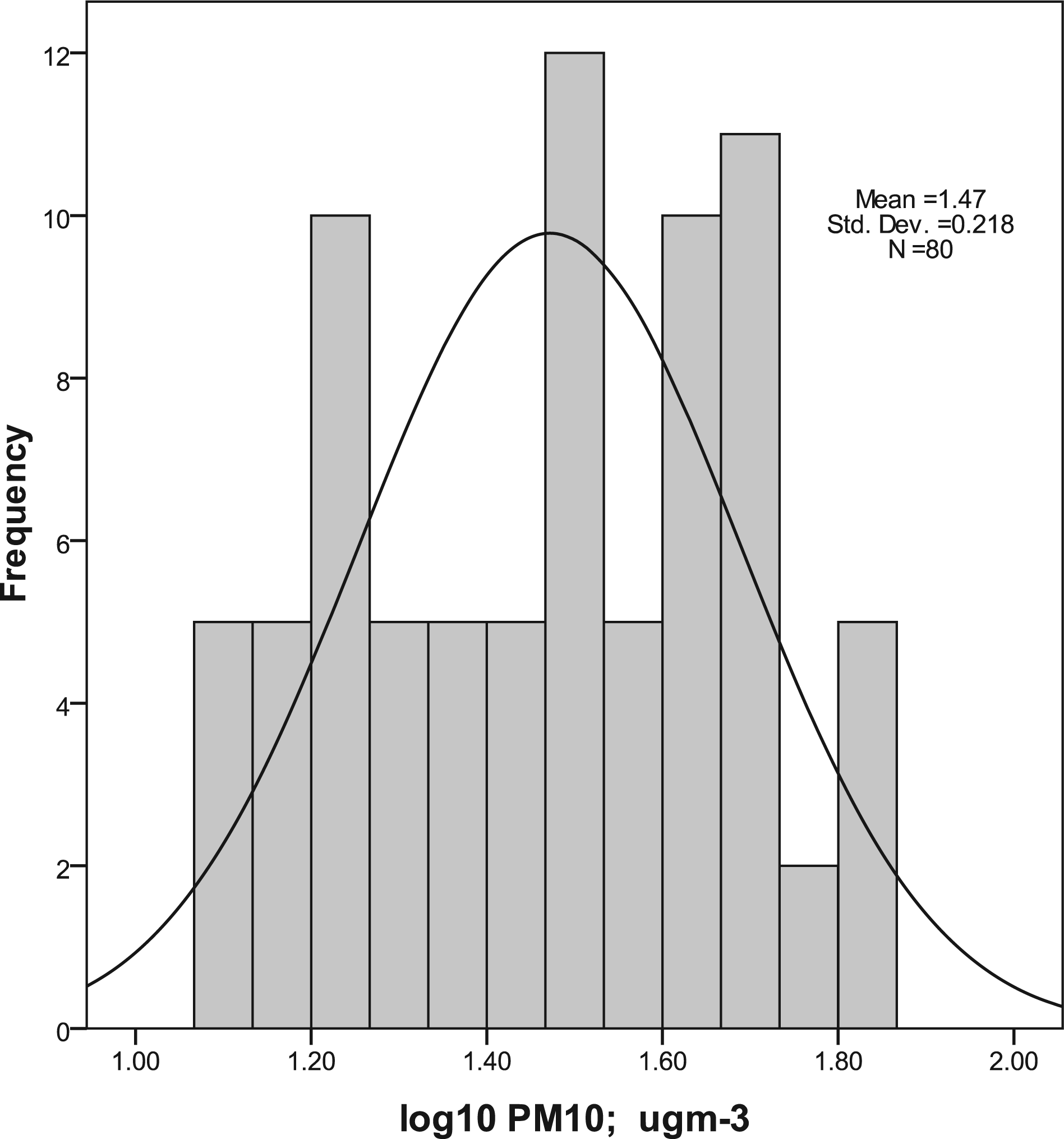

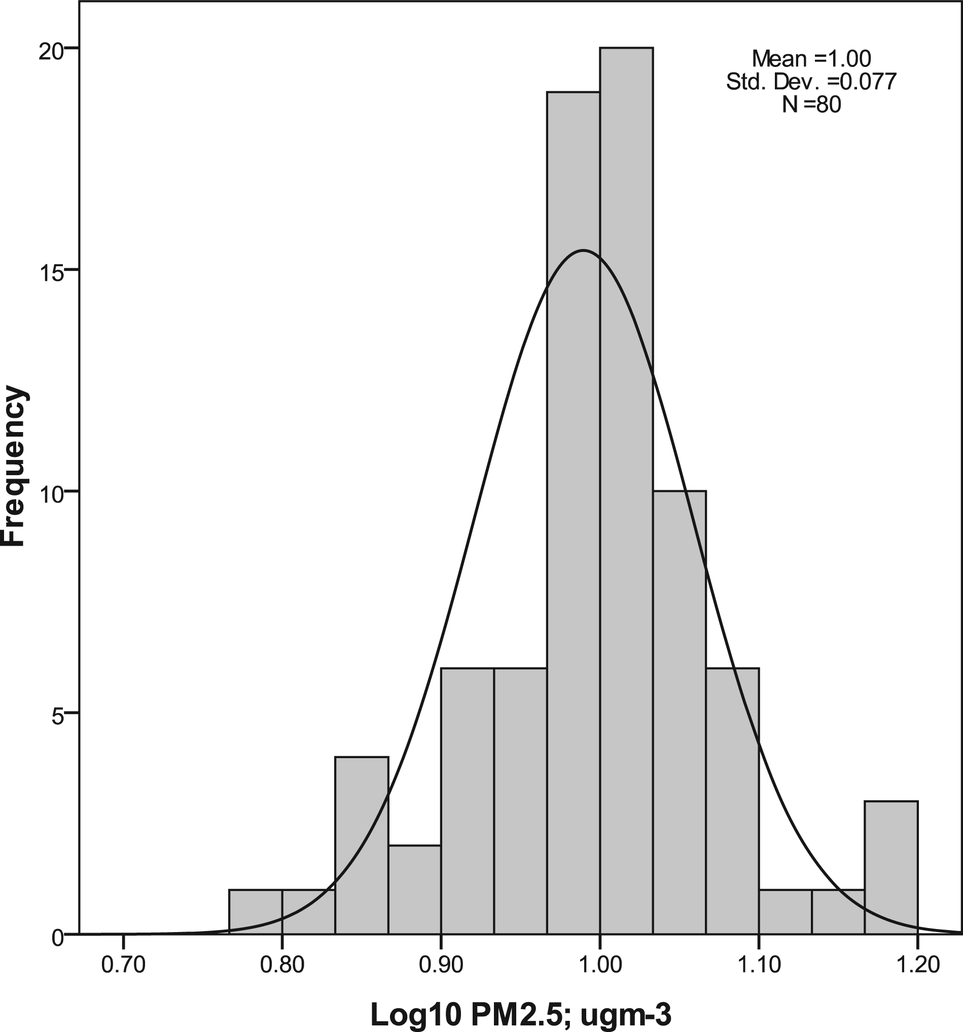
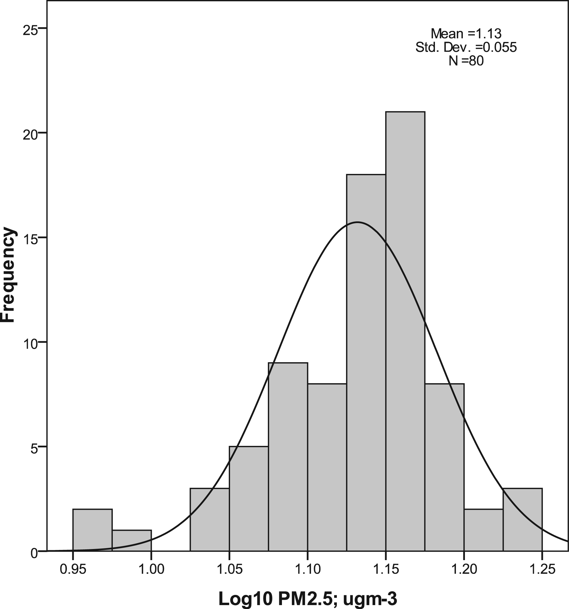
This is because some outlier subjects who formed the mode of higher personal exposure to PM_2.5 concentrations had an unexpectedly high exposure either during the daytime or leisure time. For instance, one subject had daytime and nighttime personal exposures of about 81 and 21 µg·m⁻³ during the first day and about 51 and 95 µg·m⁻³ on the second day of monitoring, respectively. This subject also spent about 6.5 h (1.75 and 4.75 h on the first and second days, respectively) in pubs and 3.2 h (2.5 and 0.75 h on the first and second days, respectively) in commuting. Whereas, this subject and other individuals who spent a considerable period of their time in polluted microenvironments showed different exposure patterns during the two monitoring days. The 24-h TWA personal exposure to PM_2.5 showed different distribution in comparison with daytime and night-time personal exposure. Subjects who showed a higher mode of TWA personal exposure spent more time in ETS microenvironments or/and travelling on the busy roads than those with lower personal exposure mode. These subjects spent 1.75–6.5 h in pubs and four subjects spent 0.5–5 h with a smoker in the same room. Two subjects that had an unexpectedly high personal exposure were living with a smoker in their homes. All highly exposed subjects, except one, spent 1.5–5 h in commuting and 5 subjects spent 0.25–2.25 h in a bus during the 48-h and monitoring period. There was no significant effect of seasons on higher weighted average exposure. The lowest exposure mode was related to six subjects who have no significant contact with cigarette smoke in pubs and their homes. Only one subject spent 45 min in a bus and most of them used their car for shorter time in comparison with highly exposed individuals.

The mean daytime personal exposure had the highest geometric mean concentration. TWA personal exposure (TWA) to PM_2.5(30.3 µg·m⁻³) showed a higher concentration than the PM₁₀ concentrations measured at the Bradford fixed monitoring station (26.3 µg·m⁻³). Geometric mean personal exposures were considerably higher in the winter than in summer. In contrast, the mean fixed site PM₁₀ concentrations were similar in both winter and summer. The personal night-time concentrations, in particular, were about twice as high in winter. The geometric standard deviation (GSD) of PM_2.5personal exposures was higher in the summer than in winter. In contrast, the GSD of PM₁₀ concentration at the fixed site was higher in the winter [8].

The univariate regression analysis showed that of 65 microenvironmental and personal characteristics included in the two questionnaires, only 9 variables including fixed site PM₁₀, road traffic, time spent in bus, smoking in the same room, smoking in different room, time spent in pub, home floor, cooking in different room and ambient temperature were significantly correlated with personal exposures to PM_2.5 measurements at p > 0.05. In contrast with other factors, such as traffic in the nearest street from home, the sizes of the houses, the height of subjects’ houses, location of the houses (urban and non-urban) and the number of office occupants, that were hypothesized to have a significant effect on personal exposure, had no significant correlation with personal exposures.

There were only weak relationships between personal exposures (daytime and night-time) and PM₁₀ concentrations monitored by the fixed site station, but maximum ambient temperature showed a significant negative correlation with personal exposures to PM_2.5 concentrations.

The multiple regression models for predicting the daytime personal exposure to PM_2.5 concentrations with fixed site PM₁₀ concentrations and microenvironmental characteristics showed that the fixed site PM₁₀ concentration and ambient temperature during the monitoring were the strongest predictors of daytime personal exposure to PM_2.5 levels (Table 1).

Table 1.

The multiple regression model of best fit for 24-h daytime personal exposure to PM_2.5with fixed site PM₁₀ concentrations and microenvironmental characteristics

Variable	Unstandardized coefficients		Standardized coefficients	t	p Value	Part correlation	Adjusted coefficient
Variable	B	SE	Beta	t	p Value	Part correlation	Adjusted coefficient
Constant	1.20	0.22		5.40	0.000
Ambient temperature	−0.01	0.01	−0.40	−2.76	0.009	−0.40	0.10
Fixed site PM₁₀	0.38	0.16	0.36	2.47	0.019	0.36	0.21

Table 2 shows the multiple regression models for predicting the 24-h night-time personal exposure to PM_2.5with fixed site PM₁₀ concentrations and other microenvironmental characteristics. Ambient temperature during the monitoring, PM₁₀ concentrations monitored by the fixed station and time spent in a pub were the strongest predictors for night-time personal exposure to PM_2.5concentrations.

Table 2.

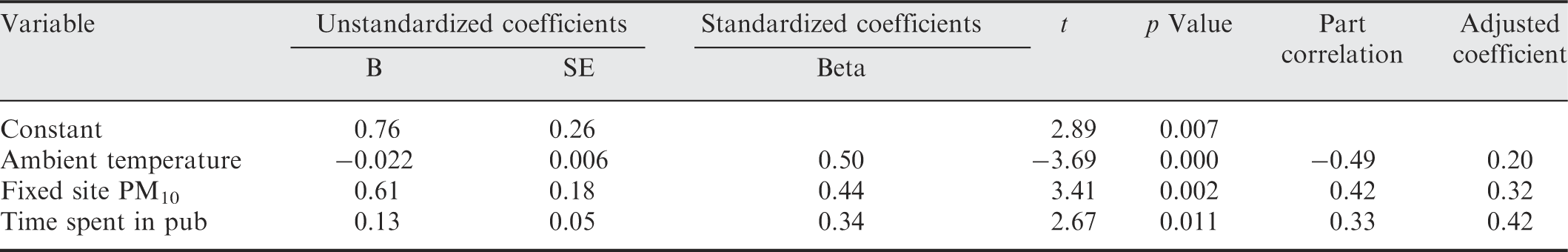
Multiple regression models of best fit for 24-h nighttime personal exposure to PM_2.5with fixed site PM₁₀ concentrations and microenvironmental characteristics

Variable	Unstandardized coefficients		Standardized coefficients	t	p Value	Part correlation	Adjusted coefficient
Variable	B	SE	Beta	t	p Value	Part correlation	Adjusted coefficient
Constant	0.76	0.26		2.89	0.007
Ambient temperature	−0.022	0.006	0.50	−3.69	0.000	−0.49	0.20
Fixed site PM₁₀	0.61	0.18	0.44	3.41	0.002	0.42	0.32
Time spent in pub	0.13	0.05	0.34	2.67	0.011	0.33	0.42

The multiple regression model analysis for 24-h TWA personal exposure to PM_2.5 concentrations as a dependent variable and fixed site PM₁₀ concentrations, ambient temperature and those microenvironmental characteristics showed a significant correlation with daytime personal exposure, as independent variables; illustrating that the fixed site PM₁₀, ambient temperature and time spent in pub and bus were the only significant predictor and about 50% of TWA personal exposure was explained by these factors (Table 3).

Table 3.

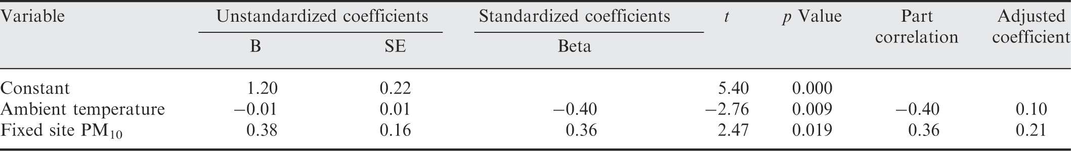
The multiple regression models of best fit for 24-h time weighed average personal exposure to PM_2.5with fixed site PM₁₀ concentrations and microenvironmental characteristics

Variable	Unstandardized coefficients		Standardized coefficients	t	p Value	Part correlation	Adjusted coefficient
Variable	B	SE	Beta	t	p Value	Part correlation	Adjusted coefficient
Constant	0.94	0.18		5.15	0.000
Ambient temperature	0.02	0.00	−0.50	−4.46	0.000	−0.49	0.20
Fixed site PM₁₀	0.50	0.12	0.46	4.04	0.000	0.45	0.34
Time spent in pub	0.12	0.03	0.41	3.57	0.001	0.39	0.48
Time spent in bus	0.15	0.06	0.26	2.34	0.025	0.26	0.54

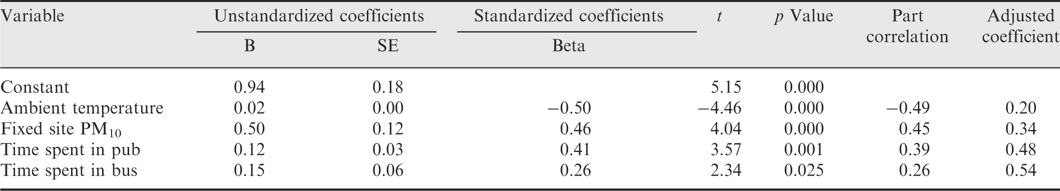
Figure 4 shows the estimated 24-h TWA personal exposure to PM_2.5 using the multiple regression models of PM₁₀ concentrations data monitored at Bradford fixed site over a year; ambient temperatures were also measured. There were higher personal exposures to PM_2.5 concentrations in the winter than those estimated in the summer. Also, range of estimated TWA personal exposure was wider in the winter than that in the summer. In contrast, FSM PM₁₀ concentrations were higher in the summer than those measured in the winter.

Fig. 4.

Estimated 24-h time weighted average personal exposure to PM_2.5 using fixed site PM₁₀concentration and ambient temperatures in multiple-regression models.

Discussion and Conclusions

The TMAD showed that more than 90% of subjects’ time was spent at home and in other indoor environments, 4.7% in travelling and about 3% outdoors. In comparison, the European EXPOLIS studies concluded that, in general, people spent 95–97% of their time indoors, 2–4% in commuting and 1% outdoors [14]. This study, compared with EXPOLIS studies, had a different method of population sampling. Participants in this study were adult volunteers (25–55 years) from non-smoking workers at the University of Bradford campus. All subjects were office workers with a little occupational exposure to particulate matter. Thus, the daytime sample in this study might be representative of occupational exposure of non-smoking adult office workers in the UK urban areas. Participants’ homes were located in the urban, suburban and rural areas of West Yorkshire. Thus, the nighttime sample in this study might represent a typical UK non-work exposure of non-smoking adult population in this area. However, the EXPOLIS studies relied on population-based sample and subjects were selected to be statistically representative of the population in each European city. Subjects were in different work positions and more likely to have some occupational exposure to particulate matter. The population sample in EXPOLIS studies included smokers and non-smokers. Hence, active smoking and exposure to environmental tobacco smoke may have had a significant effect on personal exposure to PM_2.5 in this group [6].

Although in EXPOLIS studies, personal exposure monitoring was carried out in a population-based sample including smokers, the EXPOLIS mean personal exposure over the six cities was lower than indoor office and home PM_2.5 concentrations. This was in contrast to this study, in which personal exposure was higher than indoor office and home PM_2.5concentrations. While this study measured personal exposure in the breathing zone, the EXPOLIS studies relied on equipment carried by hand by volunteers. Table 4 shows summarized statistics of personal exposures and microenvironmental PM_2.5concentrations in the EXPOLIS cities [13,15]. The geometric mean TWA personal exposure to PM_2.5concentrations in this study was substantially higher than the mean 48-h personal exposure of EXPOLIS studies in Oxford and Helsinki, and comparable to values in Athens, Basel and Prague. Also, indoor office and home PM_2.5 concentrations were higher than those values reported in Oxford and Helsinki and comparable to values in Basel. However, indoor microenvironmental PM_2.5 concentrations in this study were lower than values reported in Athens, Milan and Prague. The mean TWA personal exposure measured in this study was greater than the mean of the six EXPOLIS cities, but the mean office and home concentrations in this study were lower than the mean of the six EXPOLIS cities.

Table 4.

Mean personal and microenvironmental PM_2.5concentrations (µgm⁻³) measured in EXPOLIS studies compared to this study

Location	Helsinki	Athens	Basel	Milan	Oxford	Prague	Mean	This study
N	201	50	50	50	60	50		40
Personal Exposure	15.1	28.6	27.8	na	13.2	35.5	24.0	30.3
Indoor home	12.1	35.5	20.8	42.7	11.4	35.9	26.4	19.0
Indoor workplace	15.9	90.3	26.7	59.0	7.5	42.9	40.4	27.3
Fixed site (PM_2.5)	9.1		21.4

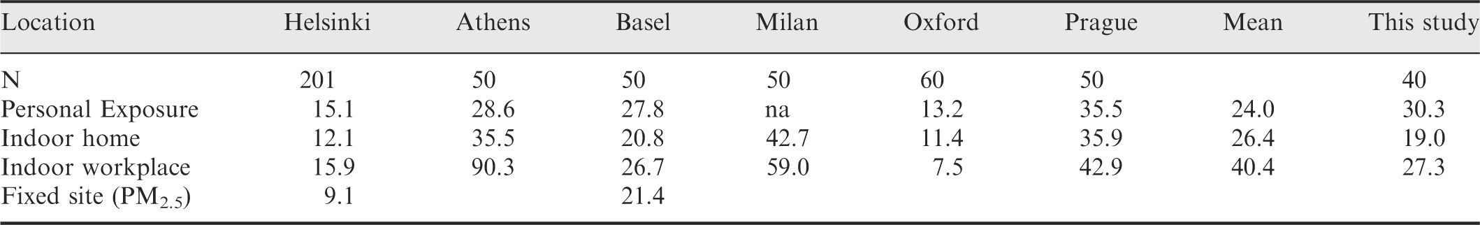
Results from this study showed personal exposures to PM_2.5concentrations that were much lower than those reported in the PTEAM pilot study (30.3 vs. 70 µg·m⁻³, respectively). However, the PTEAM pilot study was only carried out in nine homes in one month [16]. Personal exposure (TWA) PM_2.5 concentration in this study (30.3 µg·m⁻³) was similar to that reported by Pellizzari (1999) in a large-scale population study in Toronto (28.4 µg·m⁻³) [17].

In this study, via the stepwise multiple regression ambient PM₁₀ concentrations, ambient temperature and time spent in a pub were identified as predictors of nighttime personal exposure. Fixed site PM₁₀concentrations and ambient temperature were the best predictors of daytime personal exposure to PM_2.5 concentrations. The results of the EXPOLIS study in Helsinki concluded that ambient PM_2.5 concentrations and home location, as predictors of personal exposure for non-ETS participants, accounted for 47% of the variance. Time spent in a smoky pub was identified as a predictor for nighttime personal exposure [6]. Branis and Kolomaznikova also concluded that ambient data could constitute a good predictor of personal exposure and can be used for human exposure estimates [18]. The real-time monitoring in smoking and non-smoking areas in a café in this study confirmed that smoking was a significant factor causing higher indoor PM_2.5 concentrations. These results were inconsistent with those from other studies, for example Lung et al. concluded that smoking and vehicle exhaust were the two major exposure sources for PM_2.5 in coffee shops [19]. Kruize and co-workers used a simulation model in EXPOLIS studies and concluded that ETS was an important determinant of exposure [20]. This study unlike earlier studies, which did not consider this factor, showed that there were significant negative effects of ambient temperature on the personal exposure and microenvironmental PM_2.5 concentration corresponding to a given fixed site concentration. One possible explanation is that opening windows in warm weather would cause an increase in air exchange and dilution of indoor and personal exposure to pollutants when there is an indoor particle source. For example, in homes in Boston low air exchange rates (<1 h⁻¹) resulted in longer air residence times and more time for particle concentrations, generated from indoor sources, to increase; while, when air exchange rates were higher (>1 h⁻¹), the impact of indoor sources was less pronounced, and the indoors, and as a result of personal exposure to particle concentrations, tracked outdoor levels more closely [21]. However, there is no evidence of an effect of cooking on personal exposure or indoor home PM_2.5 concentrations in this study. Subjects in this study spent an average of 1 h in the kitchen during 24 h and most of them used ready-made foods, with microwave ovens being used to heat these foods in a short time. Therefore, in contrast with US studies that identified cooking as a second major source of fine particles, this study did not find any relationship between cooking and personal exposure and home indoor PM_2.5 concentrations.

Other studies found a significant relationship between personal exposure and indoor particulate matter concentrations, and some air quality-related factors such as traffic density on the nearest street from home, height of the home or office, residential locations, size of the home and number of occupants at home. Although it was expected from this study to find a relationship between these factors and personal exposure, the multiple regression analysis showed significant associations between personal exposures and these factors. This maybe because the number of subjects in this study was low (40) and the number of factors that were identified to have a possible effect on personal exposure and indoor PM_2.5 concentrations were about 65. Subjects had different personal characteristics and spent their time in different places with a wide range of microenvironmental characteristics. Thus, a small number of subjects were tested for each factor. For example, only three subjects were living in a house with an active smoker and most of those subjects that were exposed to cigarette smoke spent a portion of their time in a pub. Thus, the pub had a greater impact on nighttime personal exposure than home. Although Koistinen and co-workers have found a significant effect of home location on personal exposure to PM_2.5 concentrations in EXPOLIS study in Helsinki, this study found no correlation between home location and traffic density on the nearest street to home and personal exposure to PM_2.5 concentrations. This may be because of the small spatial variance in PM_2.5 in different locations [6]. Sokhi et al. reported from a SATERN study in London and Helsinki that the coarse fraction of PM₁₀ (PM_2.5–PM₁₀) could contribute to a higher proportion of the increased PM₁₀ at the roadside than PM_2.5, due to re-suspension of wear dust caused by the mechanical turbulence of passing vehicle [22]. No significant effect on personal exposures and microenvironmental PM_2.5 concentrations were also found from the number of occupants in homes and offices. This might be due to occupants’ activities which had caused an increase in the re-suspension of coarse fraction of particles but had little effect on fine particle concentrations.

Footnotes

Acknowledgment

We acknowledge the Iranian Ministry of Health and Medical Education and Mazandaran University of Medical Sciences, who provided financial support.

References

Schwartz

Laden

Zanobetti

: The concentration response relation between PM_2.5 and daily deaths: Environ Health Perspect 2002;110:1025–1029.

Pope

Dockery

Schwartz

: Review of epidemiology evidence of health effects of particulate air pollution: Inhal Toxicol 1995;7:1–18.

Hoek

Schwartz

Groot

Eilers

: Effect of ambient particulate matter and ozone on daily mortality in Rotterdam, The Netherlands: Arch of Environ Health 1997;52:455–463.

Katsouyanni

Touloumi

Spix

Schwartz

Balducci

Medina

Rossi

Wojtyniak

Sunyer

Bacharova

Schouten

Ponka

Anderson

: Short-term effects of ambient sulphur dioxide and particulate matter on mortality in 12 European cities: results from time series data from the APHEA project. Air Pollution and Health: An European Approach: BMJ 1997;314:1658–1663.

Wallace

: Indoor particles: A review: J Air Waste Manage 1996; 46:98–126.

Koistinen

Otto

Tuulia

Edwards

Moschandreas

Jantunen

: Behavioral and environmental determinants of personal exposure to PM_2.5in EXPOLIS – Helsinki Finland: Atmos Environ 2001;35:2473–2481.

Adgate

Ramachandran

Pratt

Waller

Sexton

: Longitudinal variability in outdoor, indoor, and personal PM_2.5 exposure in healthy non-smoking adults: Atmos Environ 2003;37:993–1002.

Mohammadyan

Ashmore

: Personal exposure and indoor PM_2.5 concentrations in an urban population: Indoor Built Environ 2005;14:313–320.

HSL: weighing stability of aerosol collections substrate, preliminary report. Health and Safety Laboratory, Wetherby, West Yorkshire, UK, 1998, pp. 1–2.

10.

DEFRA: Air pollution standards and objectives. Department for Environment, Food & Rural Affairs, UK, 2004. Available at: http://www.airquality.co.uk/archive/data_and_statistics_home.Php (accessed July 16, 2006).

11.

AQEG: Particulate matter in the United Kingdom: in Method for monitoring particulate concentrations, Air Quality Expert Group 2004; Available at: http://www.defra.gov.uk/corporate/consult/particulate-matter/index.htm (accessed September 20, 2009).

12.

Weather Underground: Temperature history for Leeds and Bradford 2002. Available at: http://www.wunderground.com/history/station/03346/2002/12/12/DailyHistory.html (accessed June 11, 2005).

13.

Lai

Kendall

Ferrier

Lindup

Alm

Hänninen

Jantunen

Mathys

Colvile

Ashmore

Cullinan

Nieuwenhuijsen

: Personal exposures and microenvironment concentrations of PM_2.5, VOC, NO₂ and CO in Oxford, UK: Atmos Environ 2004;38:6399–6410.

14.

Marino M, Carrer P, Cavallo D, Jantunen M, Katsouyanni K, Kuenzli N, Sarm R, Zmiro D, Della Torre M: Air pollution exposure of adult population in Milan (EXPOLIS study); In Levin H (ed.), Proceeding of Indoor Air‘02, 9th International Conference on Air Quality and Climate. Santa Cruz, California, July 1–7, 2002; Vol. 4, pp. 455–460.

15.

Rotko

Oglesby

Kunzli

Carrer

Nieuwenhuijsen

Jantunen

: Determination of perceived air pollution annoyance and association between annoyance scores and air pollution (PM_2.5, NO₂) concentrations in the European EXPOLIS study: Atmos Environ 2002;36:4593–4602.

16.

Özkaynak H, Spengler JD, Ludwig JF, Butler DA, Clayton CA, Pellizzari Ed, Wiener RW: Personal exposure to particulate matter: Findings from the particle total exposure assessment methodology (PTEAM) Prepilot Study; in Indoor Air '90, the fifth International Conference on Indoor Air and Climate, Toronto, Canada, July 29 – August 30, 1990; Vol. 2, pp. 571–576.

17.

Pellizzari

Clayton

Rodes

Mason

Piper

Fort

Pfeifer

Lynam

: Particulate matter and manganese exposure in Toronto, Canada: Atmos Environ 1999;33:721–734.

18.

Branis

Kolomaznikova

: Monitoring of long-term personal exposure to fine particulate matter (PM_2.5): Air Qual Atmos Health 2010; 3:235–243.

19.

Lung

Lin

: Customers' exposure to PM_2.5 and polycyclic aromatic hydrocarbons in smoking/non-smoking sections of 24-h coffee shops in Taiwan: J Exp Anal Environ Epidemiol 2004;14:529–535.

20.

Kruize

Hanninen

Breugelmans

Lebret

Jantunen

: Description and demonstration of the EXPOLIS simulation model: Two examples of modeling population exposure to particulate matter: J Exp Anal Environ Epidemiol 2003;13:87–99.

21.

Abt

Suh

Allen

Koutrakis

: Characterization of indoor particle sources: a study conducted in the metropolitan Boston area: Environ Health Perspect 2000;108:35–44.

22.

Sokhi RS, Luhana L, Kukkonen J, Pohjola MA, Kousa A, Härkönen J, Karppinen A, Aarnio P, Koskentalo T: Interpretation of atmospheric particle concentrations in London and Helsinki. A contribution to subproject SATURN Presented at EUROTRAC-2 SYMPOSIUM 2002, March 11–15, Garmisch-Partenkirchen, Germany.