Integrated building energy computational fluid dynamics simulation for estimating the energy-saving effect of energy recovery ventilator with CO 2 demand-controlled ventilation system in office space

Abstract

As ventilation is one of the critical heat loads in an office space, the ventilation rate might be optimized to develop sustainable, low-energy buildings and a healthy indoor environment. To create comprehensive and optimized indoor environmental designs, a building energy simulation (BES)-computational fluid dynamics (CFD)-integrated simulation is used to provide accurate and informative prediction of the thermal and air-quality performance in buildings, especially in the design stage. With the aim of developing an optimization procedure for the ventilation rate, this paper presents simulations that integrates BES and CFD with CO₂ demand-controlled ventilation (DCV) system, and applies them to a typical office space in Japan to optimize the ventilation rate through an energy recovery ventilator (ERV). The transient system control strategy is applied to two different airflow conditions in an office: a traditional ceiling supply system and an under-floor air distribution system. Compared with the fixed outdoor air intake rate, which is referred to as constant air volume ventilation, optimized ventilation systems associated with a CO₂ DCV produces energy savings of 11.6% and 24.1%, respectively. The difference in the energy saving effects of the two ventilation systems is caused by the difference in the ventilation efficiency in the occupied zone. The ventilation rate and ventilation efficiency have a significant impact on the energy penalty of an ERV. Therefore, optimizing the ventilation rate according to a CO₂ DCV system with an appropriate airflow pattern could contribute to both creating and maintaining a healthy, comfortable environment, in addition to saving energy.

Keywords

Building energy simulation CFD Energy saving Energy recovery ventilator

Introduction

The purpose of ventilation rate optimization in terms of indoor environment is typically for promoting energy conservation and creating acceptable indoor air quality, as well as for reducing adverse health effects, such as the symptoms of sick building syndrome. In this regard, the greatest number of descriptions is available considering optimization of the ventilation rate in office buildings. Fisk et al.¹^–⁴ noted that higher ventilation rates are associated with greater satisfaction with the indoor air environment and improved work performance. However, excess and overestimated ventilation rate, on the other hand, contributes to an increase in heating, ventilation and air conditioning (HVAC) load and high-energy consumption, consequentially raising the amount of carbon dioxide (CO₂) emitted and ultimately exerting an adverse contribution to climate change. Reducing the heating and cooling loads of buildings while taking into account the indoor environmental quality would be the most important strategy for developing sustainable buildings.⁵ In this scenario, the demand-controlled ventilation (DCV) strategy has attracted great attention owing to its potential to provide significant energy savings for buildings by adjustment of the ventilation load, in correspondence with maintenance of the contaminant concentration in the zone with occupants (hereafter, occupied zone), below a target value. Typically, CO₂, as an indicator in the indoor contamination, widely applied to indirectly measure the occupancy of a space date back to the 1970s.⁶^–¹⁰ With the potential to achieve energy savings by applying ventilation control based on occupancy or CO₂ levels,¹¹ Emmerich and Persily^12,13 provided a thorough review summarizing field measurements, analytical and numerical simulations, and sensor studies in this regard. For simplifying the discussion, most published studies and proposed methods of analysis assumed perfect and well-mixing conditions in indoors.^14,15 As a result, well-mix assumption leads to inaccurate predictions of the energy consumption of buildings that have non-uniform airflow distribution, e.g. those with displacement ventilation. In recent years, the dynamic calculation of energy consumption for a building’s thermal capacity over a longer time period, i.e. months or years, has been adopted for designing sustainable low-energy buildings.¹⁶^–¹⁸ Flow and contaminant distributions can be analysed accurately and efficiently by adopting the computational fluid dynamics (CFD) technique. Apparently, detailed information such as the airflow, temperature, and contaminant distributions, as well as details associated with heat transfer and contaminant transportation in indoor building environments can be yielded. To minimize respective deficiencies, the integration of building energy simulation (BES) with CFD would be an important tool for analyzing building energy consumption,^19,20 which takes into account information regarding the non-uniform distribution of airflow, temperature, and contaminant concentration within an enclosed space.²¹^–²⁵ However, rare integrated simulation case studies were presented and applied since the concept had been proposed as the improvement in providing accurate numerical predictions. In our previous paper,²⁶ we reported the possibility of an integrated BES-CFD simulation that could provide more accurate and informative predictions of thermal performance and an effective approach to energy conservation in a typical Japanese open-type office space. Numerical simulation analysis includes application of the energy recovery ventilator (ERV) and optimization of the layout of supply inlet and exhaust outlet openings of ERV were compared and validated with field measurements. Regarding the trade-off issue between low energy requirement and achieving acceptable indoor air quality, as our second-stage study, the performance of CO₂ DCV with ERV coupled system has been investigated by using numerical method to provide visible and reasonable indoor environment and to demonstrate the potential energy conservation of optimized ventilation system.²⁶ The present paper reports integrated simulation of BES and CFD with CO₂ DCV technology as applied to office model, and demonstrate the potential energy conservation of this optimized ventilation system. Here, an occupied space within a 1.8 -m height from the floor level is assumed as the target zone, with the aim of maintaining the CO₂ concentration below 900 ppm_v (parts per million). As the target CO₂ concentration setting, 900 ppm_v was recommended by Japanese building code and regulation^27,28 that 20 m³/h per person ventilation rate should be provided to conserve sanitary environment in the architecture for the general ventilation system design. According to EN 15251, the accepted criteria for the European, minimum ventilation rate for the breathing zone in an office is 10 L/s per person+1 L/s per m², and a minimum ventilation rate of 1 L/s m² was applied at the night time. “A level of 500 ppm_v indoors above an outdoor level 400 ppm_v would be logical,” this has been discussed in the Indoor Air Quality Guidebook by Bas Ed.²⁹

The concept of air change efficiency in an occupied zone is adopted in this study as the measure of ventilation effectiveness for optimizing the ventilation rate through the ERV. Our approach is consistent with Lawrence and Braun^30,31 that the CO₂ demand-controlled system would contribute to an effective management of spaces in which the occupants level can vary and would be especially effective when occupants levels are lower than the design levels for a given space.

Methodology

In this study, all the thermal and environmental assessments were performed using an integrated BES-CFD approach. Zhai and Chen^23,24 proposed and classified a general prediction procedure for static and dynamic coupled simulation. BES and CFD programs are adopted to take interactive complementary information for building performance prediction and evaluation into account. A transient energy simulation can predict long-term indoor environmental conditions with spatially averaged information, whilst CFD can provide relatively short-term but non-uniform distribution of the variables (See Figure 1). Step-exchange between BES and CFD is suitable for insensitive parameters in a static integration.^23,26 The executable files of complementary variants are converted to achieve integrated simulation by two steps. First, CFD is initially operated through a script file read out by a BES component. Second, CFD issues a result file, which contains information such as non-uniform scalar and vector distributions, average flow parameters in the entire room and the occupied zone as the target local domains and detailed information for each return air exhaust opening. Detailed information on the implementation of this integrated simulation is summarized in Table 1. Before conducting the simulation, CFD case based on a Reynolds-averaged Navier-Stokes (RANS) model are first run to yield a steady-state flow field by solving the transport equations of mass (continuity), the momentum of three components, and the turbulent kinetic energy and its dissipation rate. In a time series of unsteady analysis, BES is referred to as the master program of the BES-CFD integrated simulation because it governs the main timing of the continuous process in terms of thermal performance calculation. At each BES time interval, the CFD case runs under a constant boundary condition and exports non-uniform information regarding the temperature, contaminant concentration, and velocity distribution, those non-uniform data are fed back to BES when achieving a converged solution: the specified residuals and a minimum number of iterations.

Table 1.

Information for Integration simulation implementation.

Software	Exchange parameter	Export file
TRNSYS	Time-dependent feat flux Supply inlet air temperature, velocity of the ERV and PAC CO₂ generation rate	Script file
FLUENT	Exhaust outlet temperature, CO₂ concentration of the ERV Occupied zone average CO₂ concentration	Results file

ERV: energy recovery ventilator; PAC: package-type air conditioning.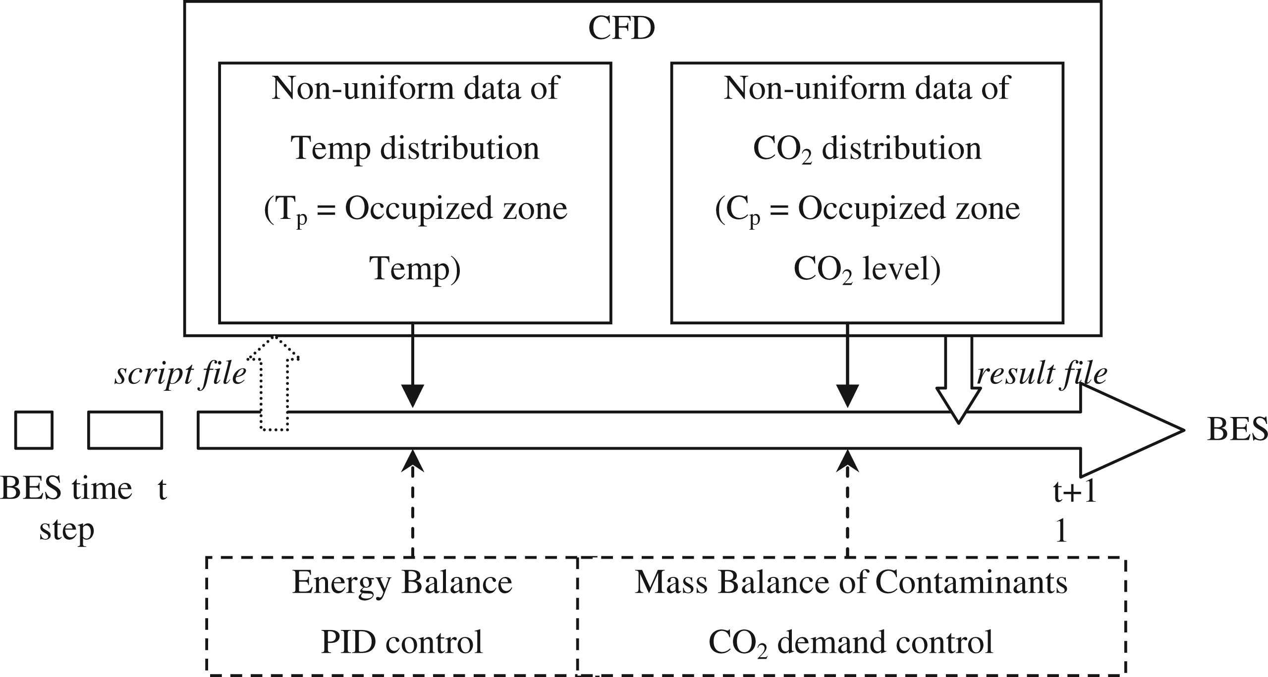

With a former determination of site-specific occupants obtained by counting the number of people every 10 min, occupants’ patterns can be estimated based on a generalized assumption of CO₂ generation rate, which is about 0.018 m³/h/person; in compliance with the design Guidebook.⁹ These are used as input boundary conditions for the integrated simulation. The source generation rate may vary throughout each BES time interval dependently.

Based on the mass balance of a single zone, ventilation rates corresponding to varied occupant densities can be judged in the evaluation of the energy savings associated with DCV as applied to the office model. In the BES simulation, the transient solution representing the indoor CO₂ concentration is identified by equation (1):

V \frac{dC}{dt} = Q_{ven} (C - C_{o}) + G_{{CO}_{2}}

(1)

We assume that the initial indoor CO₂ concentration is the same as the outdoor CO₂ concentration C_o, and the office space is then occupied with a time-varying population density of workers corresponding to the field measurement data. As shown in equation (1), the representative indoor CO₂ concentration C is determined by the ventilation rate Q_ven and the CO₂ generation rate G_co₂ owing to the occupants. Under a steady and equilibrium condition, a perfect mixing concentration C_e is defined by equation (2).

C_{e} = C_{o} + \frac{G_{{CO}_{2}}}{Q_{ven}}

(2)

where C_e is the equilibrium concentration (perfect mixing concentration), C_o is the outdoor concentration, and G_co₂ is the CO₂ generation rate. Q_ven represents the steady-state ventilation rate for the office space.

Various types of indices for ventilation efficiency and ventilation effectiveness have been proposed. Here, the ventilation effectiveness is defined by equation (3), as originally presented by Sandberg,³² and this was used for optimizing the ventilation rate. Ventilation effectiveness E in equation (3) is defined as the ratio between the averaged concentration of the occupied zone and that of a perfect mixing condition.

E = \frac{C_{e} - C_{o}}{C_{p} - C_{o}}

(3)

The reference C_e denotes the concentration at the exhaust opening, which is considered to represent the perfect mixed concentration of contaminants in space. C_p indicates the point concentration, here represents the local domain (the occupied zone within 1.8 m height from floor level) concentration in target space. In this sense, E corresponds to the normalized concentration in an occupied zone, which has been defined as a ventilation index in The Society of Heating, Air-Conditioning and Sanitary Engineers of Japan (SHASE) Standard 102. C_o refers to the supply air concentration through the ERV, which corresponds to the outdoor air concentration. This ratio is referred to as the ventilation effectiveness, which indicates how efficiently the outdoor air is distributed to the target local domain in a room.

The air change efficiency ɛ can be defined by the ratio of the local age of air τ_p and the nominal time constant τ_n. This definition was introduced in ASHRAE Standard 62.1:2010, and the measurement procedure is also given in ASHRAE Standard 129:1997 (RA2002) for measurement of air-change effectiveness.³³

ɛ = \frac{τ_{n}}{τ_{p}}

(4)

With CFD simulation, the scale of ventilation efficiency (SVE3) presented by Kato³⁴ was used to estimate the local age of air by discretizing the scalar transportation equation with uniform contaminant generation. In this numerical procedure, the contaminant is generated uniformly and continuously throughout the occupied zone as initial condition. On the basis of the spatial distribution of a three-dimensional flow field, the non-uniform distribution of the age of air can be analysed. In other words, ventilation effectiveness E defined in equation (3) and air change efficiency ɛ in equation (4) are the expressions of the same physical phenomenon by a different aspect.

In this paper, in order to estimate the general ventilation efficiency of an office space, the age of air distribution and air change efficiency ɛ defined in equation (4) are adopted. In our study, the ventilation effectiveness E defined in equation (3) was used for optimizing the ventilation rate by employing a CO₂ DCV procedure.

Here, we assumed the non-Reynolds number dependence of the flow and contaminant distribution within one time step (dt) from tⁿ to tⁿ⁺¹. Thus the ventilation effectiveness E was kept constant while CFD implementing under steady state condition within each time step d_t. In addition, the ventilation rate of the next time interval was adjusted and updated by E, as shown in equation (5).

E = \frac{C_{ext}^{n} - C_{o}}{C_{p} - C_{o}} = \frac{C_{ext}^{n + 1} - C_{o}}{C_{tag} - C_{o}}

(5)

where the C_tag indicates the set-point concentration (ppm_v).

In our numerical simulation, with a known initial condition, the steady-state ventilation rate was solved by introducing a constant ventilation effectiveness E estimated by CFD simulation within each time step as follows. A minimum ventilation rate Q_min of 158.4 m³/h (corresponding 1 l/s m²) was applied during the night time.^35,36 Minimal ventilation rate was used as night-purge ventilation (NPV) to flush warm air out of the building and cool thermal mass for the next day. Basically, mechanical ventilation would efficiently remove and exhaust VOCs, which would continuously emit and accumulate in the office space. The upper and lower constraints of the ventilation rate are shown as follows:

Q^{n + 1} = \frac{C_{p} - C_{o}}{C_{tag} - C_{o}} Q^{n} = Q^{n} + \frac{C_{p} - C_{tag}}{C_{tag} - C_{o}} Q^{n} (8 : 00 - 18 : 00)

Q^{n + 1} = Q^{n} = Q_{\min} (18 : 00 - 8 : 00)

(6)

Application to simulation

CFD model

The BES-CFD integrated simulations with a CO₂ DCV system were carried out for an open-type office space located in Gifu prefecture, which has a mild climate in Japan. ANSYS/FLUENT 12 was adopted as commercial CFD software. First, the CFD numerical model was prepared to provide detailed data on the flow field, for predicting transient variations in the CO₂ levels of the occupied space under realistic operating conditions. The target office space was the ground floor space of a two-storey office building with dimensions of 28.225 m (x) (length) × 15.45 m (z) (width) × 2.4 m (y) (height). Unstructured grid with size function was adopted to configure the desks, internal partitions, and bookshelves, giving a total of 703,180 cells that were arranged inside the office model. Considering the time consuming integrated simulation, this grid resolution is in compliance with the guidebook³⁷ given for typically sufficient number of cells for the corresponding room size (Formula derived for the German guideline VDI 6019). A cutaway view of the physical model is presented in Figure 2.

The configuration is described as consisting of a main open working space and two fitting rooms. Representative double-glazed windows were set on the north and east walls of the main office space. The office space was hypothetically separated into two zones: an occupied zone with 1.8 m (y) height from the floor, which was targeted for time-depended CO₂ generation assuming a constant human metabolic rate. Conditioned air was provided by a package-type air conditioning (PAC) system located at the ceiling, so the air supplied through the PAC system was distributed indirectly to the occupied zone through the upper ambient zone. The supply and return openings of the ERV system were arranged on the ceiling plane so that outdoor fresh air was supplied directly to the upper zone of the office space. With a supply jet diffuser and return vents on the ceiling, a detailed evaluation of the fluid flow, heat transfer, and contaminant diffusion in the office could be analysed by discretizing the numerical model.

In this study, the flow pattern in the office space was analysed by using a standard k-ɛ turbulence model with generalized log-law-type wall functions, and the logarithmic law for mean velocity which is known to be valid for 40 <y⁺ (wall unit) <130 in the turbulent region where effects of turbulence would dominate conduction.³⁷ Extensive research^38,39 had demonstrated that the airflow and turbulence features in an enclosed environment could be calculated by RANS models with acceptable computing cost and accuracy. The air movement was yielded from discretizing mass, momentum, and energy equations using a finite volume method. Steady state and three-dimensional analyses were conducted. Heat transfer at wall surface was mainly by convection and radiation, respectively. With calculation of view factor, the surface-to-surface (S2S) radiation model of ANSYS/Fluent was employed to account for the radiation exchange in a spatial enclosure of gray body surfaces. To obtain a solution for the discretized Navier-Stokes equations, SIMPLE algorithm and second-order upwind scheme were applied in the CFD simulation. The buoyancy models that employed the Boussinesq approximation, based on the assumption that the fluid density was a function of temperature, were also integrated. The normalized residual was set at a level of 1 × 10^–8 (refer to in Appendix 1 for grid independent check).

When reproducing a reliable air movement, appropriate initial conditions and boundary conditions were the required components to be applied. Supply inlet boundary of conditioned air through the package air conditioner (PAC) was considered as a constant air velocity boundary. In other words, the PAC operated and processed indoor air with a constant airflow rate. The air temperature at the supply inlet was specified via proportional-integral-derivative (PID) controlled technique components of the BES software. The airflow velocity, concentration level, and the turbulence quantities provided through the ERV was set in accordance with the adjusted solution of CO₂ demand control procedure. In order to model outflow, we applied free slip (gradient zero) boundary conditions to exhaust openings of the PAC and ERV.

Using a scalar transport equation, the heat and mass transfer, including convection and diffusion, and the non-uniform distribution of the target scalar could be analysed simultaneously. Equation (7) indicates the transport equation of the relevant scalars, e.g. temperature, humidity, and CO₂.

\frac{\partial Φ}{\partial t} + \frac{\partial \bar{U_{i}} Φ}{\partial x_{i}} = \frac{\partial}{\partial x_{i}} ((Γ + \frac{μ_{t}}{σ_{t}}) \frac{\partial Φ}{\partial x_{j}}) + S_{Φ}

(7)

where

\bar{U_{i}}

is the ensemble averaged air velocity vector, Φ is the target scalar, Γ is the molecular diffusion coefficient of the target scalar in air, μ_t is the turbulent viscosity,

σ_{t}

denotes the Turbulent Schmidt number, and

S_{Φ}

refers to a source term.

The heat sources represented by the working appliances such as personal computers and other devices were assumed to be uniformly distributed on the desk and table tops. This heat generation was also made to vary according to the occupants’ pattern, as shown in Figure 3. Uniform distribution was also assumed for the heat generated from lighting devices on the ceiling. The CO₂ was generated volumetrically as an average for the occupied zone corresponding to variations in occupant density, and it was assumed that a constant concentration of outdoor CO₂ was introduced through the supply opening. With regard to the CO₂ generated by the occupants, within the occupied zone, we assumed a uniform generation of 0.018 m³/h per person as the CO₂ generation rate under the conditions of a light-working situation, as the source term of equation (7). The CO₂ concentration threshold of the occupied zone was set and targeted at 900 ppm during the work period by adjusting the ventilation rate in correspondence to the variations in CO₂ generation during each BES time interval (1 h).

BES model

All the thermal characteristics of the building’s performance and energy recovery efficiency produced by the ERV system were represented by BES components (TRNSYS). Thermal performance and contaminant concentration control procedures that corresponded separately to energy and indoor air quality evaluations were taken into account in this integrated system design. With a view to control the energy consumption, ERV and CO₂ DCV system were installed. Simultaneously, the spatial indoor air quality was controlled by a CO₂ DCV system through the ERV.

With regard to thermal-performance-controlled systems, ERVs were employed for the exchange and recovery of sensible heat between the outdoor and indoor air. In this study, humidity as a form of latent heat was disregarded. Furthermore, a PID controller (Type 23) was applied to minimize the temperature fluctuation of around 28°C in the occupied zone by adjusting the process supply air temperature of the PAC system. The adiabatic ERV system was composed of a heat exchanger (Type 91) and ducts (Type 31), whose temperature exchange efficiency of 60% was validated as being in accord with the field measurement data.

The unsteady CO₂ concentration was calculated using a mass balance equation at each time step, and the ventilation rate through the ERV was updated using the concept of ventilation effectiveness E that was estimated by the CFD simulation. A constant and minimum ventilation rate of 158.4 m³/h was assumed during the night to maintain a minimum air quality and to anticipate the night purge effect.

In TRNSYS, a multi-zone building module (Type 56) was used to predict the transient thermal behaviour of both the individual components and the ventilation system. Based on real climate conditions, meteorological data obtained from Meteonorm were chosen for setting the BES boundary conditions. Detail description of building component properties and environmental information are shown in Table 2. To exchange information with the CFD software, an original macro program defined as Type 306, which was originally created by Diego for transporting mutual complementary boundary conditions, was adopted for the calculation strategies in this optimized integrated system.

Table 2.

Analysis parameters of BES.

Meteorological data	Meteonorm Matsumoto		CHTC	Wall	Front 7.2 kJ/h m²K; Back 1000 kJ/h m²K
Simulation period	September 4th–7th		CHTC	Window	Front 11 kJ/h m²K; Back 64 kJ/h m²K
Time step	1 hour		Solar absorbance		0.8
View factor to sky	0.5		LEC of wall		0.9
Heat generations	Human body	100 W/person	Enclosure behaviour		Outwall u-value	0.344 W/m²K
	PC & device	140 W/each			Intwall u-value	2.194 W/m²K
	illumination	10 W/m²			Floor u-value	0.721 W/m²K

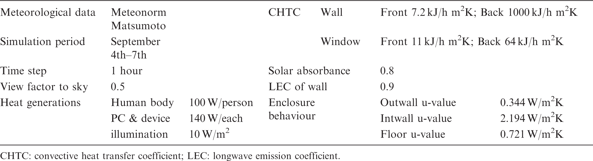
CHTC: convective heat transfer coefficient; LEC: longwave emission coefficient.

Cases analysed

To evaluate the potential preponderance of the DCV system in reducing energy consumption, two representative cases were established for numerical analysis: (i) a traditional ceiling supply of the EVR with CO₂ demand control and (ii) an optimized floor supply of the ERV with CO₂ demand control. In this study, Case 1 is referred to as the basic constant volume ventilation case, which was estimated using a BES only simulation. To emphasize the advantage of the integrated simulation, this unique case was carried out only for estimating the energy consumption. Table 3 presents detail analysis for each case. In Case 2, the ventilation supply inlet openings were set at the ceiling in the perimeter zone, in accordance with real office conditions. In Case 3, the supply inlet openings were arranged at floor level and the exhaust outlet opening at the ceiling, to create a quasi-displacement ventilation system. Eventually, two DCV cases were established to quantitatively compare the energy conservation, airflow pattern, and CO₂ concentration distribution to demonstrate in terms of different supply inlet/exhaust outlet arrangements of the ventilation system.

Table 3.

Cases analysed.

Case	Approach	Symbol	ERV		Night ventilation	Control target
1	BES	CAV_BES	Ceiling supply	CAV	Off	Entire perfect mixing	PID 28°C
2	BES-CFD	DCV_cn	Ceiling supply	DCV	On (1 l/s m²)	Average temperature in occupied zone (1.8 m)
3	BES-CFD	DCV_f	Floor supply	DCV	On (1 l/s m²)	Average temperature in occupied zone (1.8 m)

BES: building energy simulation; CAV: Constant air volume; CFD: computational fluid dynamics; DCV: CO₂ demand controlled ventilation; ERV: energy recovery ventilator; PID: proportional-integral-derivative.

Field measurement

Field measurements were performed for confirming the numerical simulation results to quantify energy savings associated with the application of the CO₂-demand-controlled strategies. The major aim of field measurement and comparison with numerical simulation results in this study was extraction of the controversial points in numerical method. In the testing office site, a total of four ERV units were set in the ceiling, each of which provided a rated air volume of 350 m³/h. The airflow velocity, temperature, and amount of CO₂ were measured at specific locations in the office (see Figure 4).

Table 4 summarizes the properties and the accuracies of the experimental apparatus. One of the CO₂ sensors was randomly placed at the return opening of one ERV, which represented the perfect mixing location, as reported in extensive experimental studies.^8,40^–⁴¹ The other CO₂ sensor was secured and positioned at a height of 1.5 m in the centre of the office space. As shown in Figure 4, the indoor CO₂ concentration was investigated and recorded by a multi-gas monitor (INNOVA) that has an error range of ± 5%. The strategy of the CO₂ DCV used in the site measurements did not perfectly correspond to the integrated simulation of BES-CFD and CO₂ DCV. The CO₂ DCV system in the field measurements adopted a multi-stage procedure for optimizing the ventilation rate. More specifically, two stages of the ventilation rate of each ERV, i.e. Q₁ = 588 m³/h and Q₂ = 1155 m³/h, were selected in incremental steps to achieve a CO₂ concentration of 900 ppm. This feedback of the optimization of the ventilation rate was executed at a frequency of 5–6 times an hour.

Table 4.

Instrumentation used in field measurement.

Measurement	Apparatus	Detection limit accuracy	Minimal logging interval
Air temperature/humidity	Resistance (RTD) Sensor Electronics, LR5001	–40.0−85.0°C ± 0.5°C	1 min
CO₂ concentration	Photoacoustic Multi-gas Monitor 1312, CO₂ Engine™ K30	0−2000 ppm_v ± 150 ppm	20 s
Ventilation rate	Air volume meter, SWF-125	7.2−450 m³/h ± 0.5%	1 s
Energy consumption	Remote measurement System 2331	AC 100/200 V AC 5−500 A ± 1%	1 min

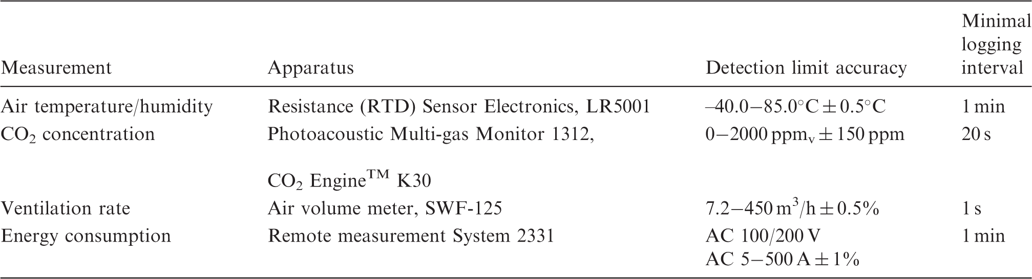
The measurement data consisted of the return and ambient air CO₂ concentration along with the outdoor air damper position. The amount of outdoor intake air was a function of the outdoor air damper position, which was adjusted by the indoor testing CO₂ concentration. In these site measurements, the night purge with a minimum ventilation rate was not implemented during periods of non-occupancy. The occupants associated with the CO₂ source generation rate were derived in this investigation by counting the number of persons within the field site.

Various uncertainties were included in this field measurement and there was a constant difference with the boundary conditions of the BES-CFD integrated simulation with CO₂ DCV. Nevertheless, the field measurement could provide informative data to evaluate the prediction accuracy of numerical simulation in view point of the overall trend and order estimation.

Results and discussion

In this study, BES-CFD with CO₂-based demand-controlled integrated simulation was carried out basically to correspond with field measurement scenarios. The impact of different ventilation opening positions on the energy cost saving in the office model was also investigated. Additionally, comparison between simulation and field measurement was provided for engineering application confirmation.

Application evaluation of CO₂ DCV often involves predicting the energy consumption for both optimized ventilation and fixed ventilation (a constant air volume (CAV)). Therefore, two cases of CO₂ DCV integrated BES-CFD simulations with different supply opening positions of the ERV were conducted to compare results with the case obtained using a fixed ventilation. Here, detailed three-dimensional information of the dynamic airflow and scalar distributions are discussed in terms of the trade-off between energy saving and indoor environmental quality. Case 1 was treated as the baseline, with the fixed outdoor intake rate as the original CAV ventilation. In Case 2, the DCV supply opening at the ceiling was set up in the interior zone to reflect the arrangement in the existing office. In Case 3, DCV floor supply case, the supply opening was arranged under the floor to maximize the use of the natural thermal effect of the existing space. The energy saving potential associated with CO₂ DCV as applied to different supply opening locations was evaluated by a comparison with the CAV ventilation system referred to in Case 1, with the aim of analyzing the fresh air load reduction achieved through the ERV system.

Flow, temperature, and CO₂ concentration distributions

Examples of the prediction results for the airflow parameters used in the estimation of the indoor thermal environment and air quality, i.e. temperature, airflow, and CO₂ concentration distributions, are shown in Figure 5. Horizontal cutaway views at a height (y) of 1.5 m and a vertical section at the centre of the office model are presented. These results indicate three-dimensionally the non-uniformity of the distribution of flow, temperature, and CO₂ concentration in space. In accordance with real conditions, the office was geometrized for the CFD analysis, and the specific temperature distribution patterns indicate that the temperature of the occupied zone basically complied with the controlled target of 28°C. Thermal stratification and significant non-uniform temperature distribution in the office space appears on the vertical profile. This obviously shows that high-temperature air accumulates in the upper ventilated zone, especially around the ceiling. The average air velocity at the centre of the office space was about 0.2 m/s, and a draught flow field with a relatively high air speed was formed locally in the vicinity of the PAC system in the office space. The CO₂ levels are non-uniformly distributed in these horizontal and vertical sections. The target CO₂ concentration level of 900 ppm_v in the occupied zone was used to determine the ventilation rate. Thus, the average CO₂ concentration in the occupied zone was controlled at approximately the target concentration level, but with approximately 20% differences in the CO₂ concentration at each point or in each local domain.

Comparison with traditional fixed ventilation and optimized DCV

To estimate a building’s performance in terms of its potential to achieve reduced energy consumption via a CO₂ DCV system, a BES-CFD integrated simulation was carried out to predict the energy costs for both the case of fixed ventilation with a CAV (Case 1) and that of demand ventilation with a variable air volume, to maintain the CO₂ level within the target zone (Cases 2 and 3). In addition, to analyse the optimized ventilation quantitatively, different supply air opening locations, which are referred to as traditional ceiling supply (Case 2) and under-floor supply (Case 3), were compared, using the distribution of airflow parameters with the same thermal behaviours in a typical building.

Removal efficiency of CO₂ generated indoors

As shown in Figure 6, the time series of the average CO₂ concentration (C_{ave_cn}) of the occupied zone are of a similar order, compared with the traditional ceiling supply (Case 2) with the C_{ave_f} under-floor supply (Cases 3). This indicates a reasonable effect of the application of the CO₂-demand-controlled strategy in both cases. In Case 2, the return air concentration (C_{RA_cn}), which represents the perfect mixing concentration, is relatively lower than C_{ave_cn}, the average CO₂ concentration in the occupied zone, during the period of work. In other words, the occupied zone is more contaminated than the upper ventilated zone. The reason for this is that the outdoor air supplied through the ceiling supply openings was diffused in the upper zone but was not effectively transported to the occupied zone. On the other hand, in Case 3, the under-floor diffuser system could supply outdoor air to the occupied zone and could employ the buoyancy forces more efficiently to remove contaminants from the occupied zone.

Figure 7 shows comparisons between the average CO₂ concentrations of a horizontal plane at specific heights of the vertical space for the traditional ceiling supply (DCV_{_cn}) and the under-floor supply (DCV_{_f}). The figure also shows plots of the horizontal plane averaged CO₂ concentrations at intervals of 0.5 m from floor level. Figure 7(a) shows a comparatively large disagreement with the values for the 1-m height above floor level, which is caused by the fresh air intake from the under-floor diffusers, and directly purged contaminant close to floor level, in the case of under-floor supply (DCV_{_f}). In addition, in the initial operating hour for the ERV in the morning (8:00), the upper-side concentration of the ceiling supply and the under-floor supply cases show good agreement with each other. Figure 7(b) shows relatively good purging efficiency of the CO₂ generated in the occupied zone in the floor-supply case, at noon (12:00). This trend is caused by the quasi-displacement ventilation of the airflow, which moves the contaminant upwards, driven by buoyancy forces. With regard to air quality, the under-floor-type ventilation system can provide fresh outdoor air directly into the occupied zone, thus generalizing a distinct difference in the vertical concentration profiles, in contrast to the traditional ceiling supply system with its well-mixed ventilation. In the ceiling supply case, on the other hand, the return air concentration is relatively lower than the CO₂ concentration of the occupied zone because of the lower efficiency of the air change. In Figure 7(c), we see that in the late afternoon (16:00) there are relatively similar CO₂ levels and vertical distributions in both cases. Clear vertical distributions of the CO₂ concentration were not confirmed at 16:00, except in the vicinity of the floor. However, in the occupied zone (1.8 m above the floor), the CO₂ concentrations in Case 3 of the under-floor supply condition are lower than that in Case 2 of the ceiling supply condition at each height level, and they are inverted at the exhaust opening level owing to the direct outdoor air supply from the ceiling in Case 2.

In Figure 8, the mean age of air in the occupied zone corresponding to its nominal time constant value at three specific hours, i.e. 8 AM, 12 AM, and 4 PM, are shown. In the ceiling supply cases (DCV_{_cn}) in Case 2, the ventilation effectiveness E values defined in equation (4) are 0.99, 0.95, and 0.94, with nominal time constants of 0.77, 0.94, and 1.10 h, respectively. This means that the mean ages of air in the occupied zone are greater than the nominal time constants and that the ventilation efficiency is responsible for the perfect mixing condition. In Case 3 of the under-floor supply condition, the ventilation effectiveness values are 1.01, 1.01, and 1.02, respectively, for nominal time constants of 0.68, 0.96, and 0.88 h. In addition, all the values for the mean age of air are lower than 1.0, results indicate that the floor-supply airflow characteristics purge contaminants more efficiently in the occupied zones. Compared airflow supply rate with PAC, one-tenth of total conditioning airflow amount was supply through ventilation system. Therefore, mixing effect, air jet from ceiling through PAC system, was dominant in office model.

Figure 9 shows the differences in ventilation effectiveness, which are referred to as the ratio between the perfectly mixed CO₂ levels and the occupied zone’s average CO₂ concentrations in two cases (Cases 2 and 3). The ventilation effectiveness values in Figure 8 are estimated using the definition in equation (3), and they consider the non-uniform generation of CO₂ in the target space. Here, we adopt the occupied zone average CO₂ concentration as the target concentration for computing the ventilation effectiveness. On the other hand, the ventilation effectiveness in equation (4) indicates the general ventilation performance, under the assumption of uniform contaminant generation within the entire target space. The ventilation effectiveness in equation (4) becomes only a function of the airflow distribution. Thus, the effect of the source location as a limitation is ambiguous. The results in Figure 9 indicate that the ventilation effectiveness (E in equation (3)) in the ceiling-supply case is constantly lower than it is in the under-floor supply case, based on a similar average CO₂ concentration in the occupied level, and that it remains approximately constant at all times from 8:00 to 18:00. This means that the Reynolds number dependence of the flow field in the target office space is almost negligible, and thus, the application of Equations (5) and (6) in the optimization of the ventilation rate is reasonable for this analytical condition.

Time series of indoor distributions of airflow parameters

Figure 10 shows the CFD results for airflow, temperature, and CO₂ concentration distributions in Case 2 obtained for traditional ceiling supply integrated CO₂ DCV and a time series of the non-uniform prediction results of scalar and vector obtained with the BES-CFD integrated simulation. A 1.5-m-high cutaway section and four representative time intervals (8:00, 12:00, 16:00, and 20:00) are presented.

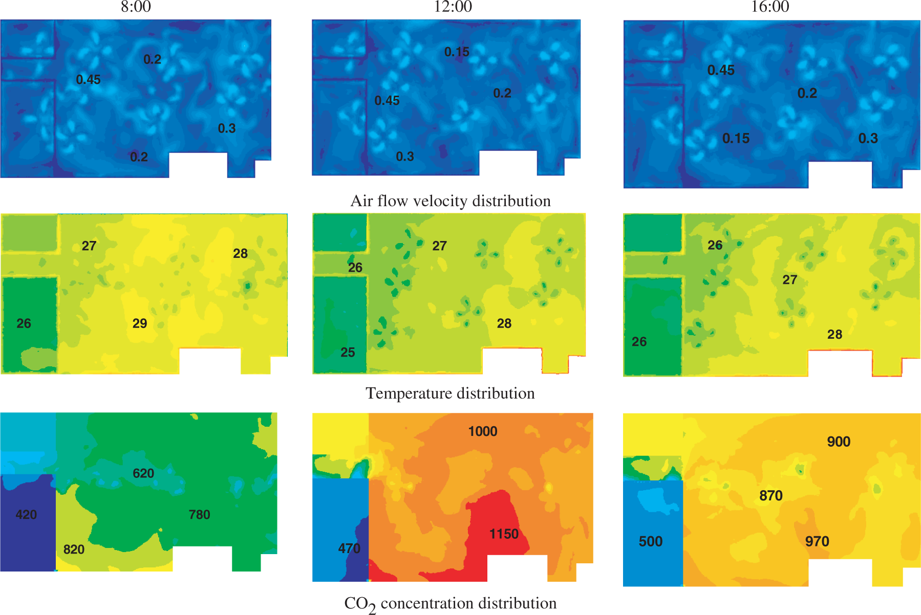
In particular, PACs were operated at the ceiling level in both cases, and they had a significant impact on the airflow patterns in the office space. The average air velocity at the centre of the office space was about 0.2 m/s, and similar velocity profiles were formed in the horizontal plane at each time interval. Because of an approximately constant density of worker occupancy and the continuous operation of electrical devices, the temperature distributions in the workspace became almost stable and were uniformly distributed to achieve the target temperature for PID control (28°C) during work periods. A high CO₂ concentration region in the office space was produced that corresponded to the highest density of occupancy at the peak time of around noon (12:00). These comparisons were made using the estimated occupancy that was derived from the preliminary investigations of the field measurements. As a consequence of this study, the peak CO₂ level displayed dependence on the CO₂ generation rates as a source term, and it had a stronger impact on the time series CO₂ concentration distribution than the distribution of ventilation effectiveness.

Figure 11 shows time series of the airflow, temperature, and CO₂ concentration distributions in Case 3 obtained with under-floor supply integrated CO₂ DCV. Compared to the ceiling-supply condition, in Case 3 with under-floor supply ventilation there was no critical difference in the velocity distribution in the occupied zone, owing to the effects associated with mixing by the PAC system. With regard to the temperature distributions, a high-temperature zone was confirmed in the vicinity of the ceiling and desk surfaces owing to the heat source indoors. The target office space was well insulated, and thus, this boundary condition had a dominant impact on the temperature distributions in the perimeter zone of the office space.

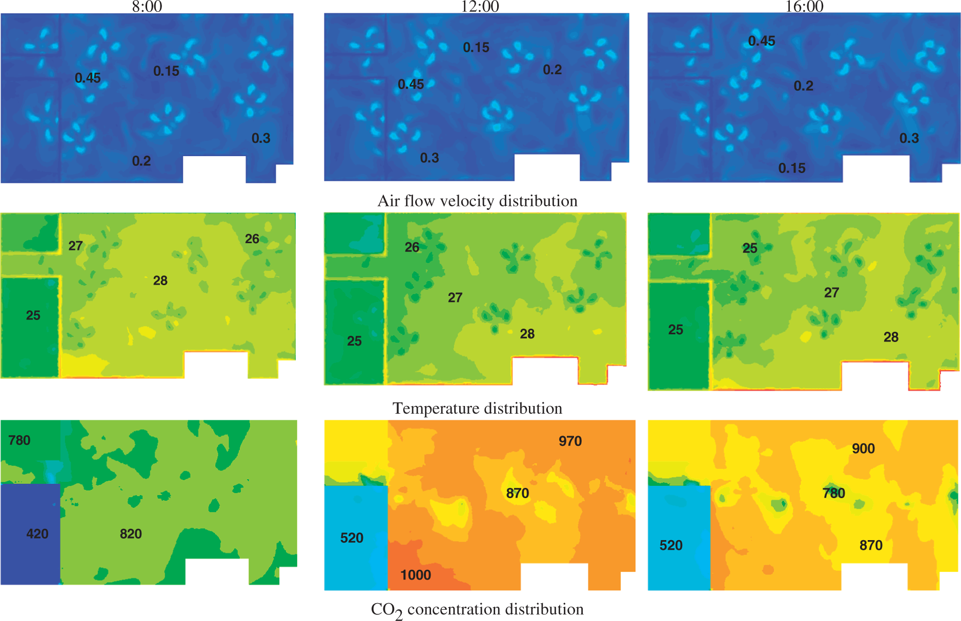
Compared with the two types of ventilation systems from the viewpoint of CO₂ concentration distributions, the CO₂ concentration in Case 3 with the under-floor supply type was relatively lower than that in Case 2 with a ceiling-supply type, which indicates the relatively superior ventilation effectiveness of Case 3.

Estimation of ventilation rate and energy cost saving

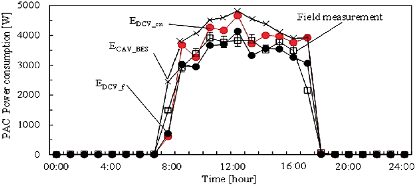
Figure 12 shows a comparison of the ventilation rates for the two DCV cases with different supply opening positions (Cases 2 and 3) and for the fixed ventilation rate condition (Case 1). Q_CAV_{_BES} in Figure 12 indicates the ventilation rate of the BES-alone case that takes into account the energy prediction. The average outdoor intake rates produced by the two DCV cases (Q_{DCV_cn} and Q_{DCV_f}) are lower than that of the fixed ventilation case (Q_{CAV_BES}). As shown in Figure 13, the ceiling-supply DCV case could save 11.58% more energy than the fixed ventilation case. The performance of this under-floor supply case with optimized ventilation associated with the CO₂ DCV strategy could lead to minimization of the energy penalty by 14.1% as compared to the ceiling-supply case, and it was able to reduce it by approximately 24.1% as compared to the fixed ventilation case. If we ignore the entire morning period in which the ventilation rates fluctuated and focus on the afternoon period, the CO₂ DCV system in Cases 2 and 3 could contribute to a reduction in energy consumption by 30% and 38.5%, respectively, as compared to Case 1. At the same time, the floor-supply system was superior to the traditional ceiling-supply case, displaying a 12.2% greater energy-saving performance. BES-alone case underestimates the energy power consumption by 10%–15%, compared with field measurement data.

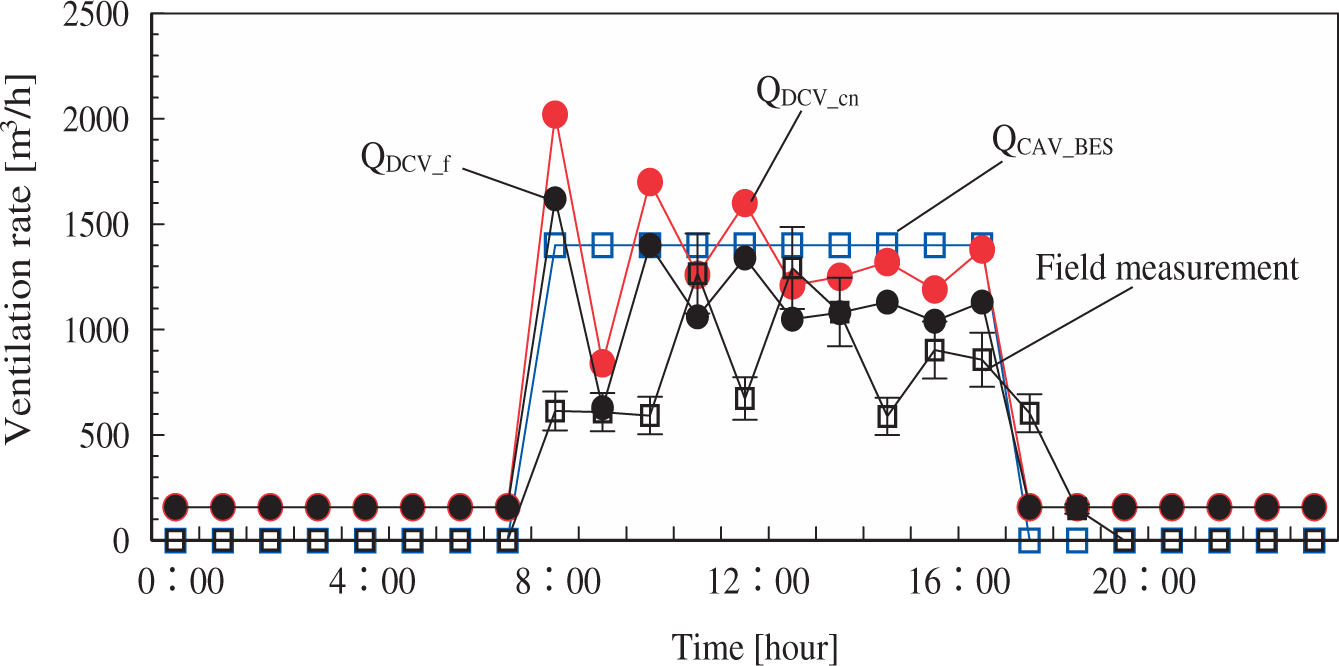
Comparison between field measurement and numerical prediction

Ventilation rate prediction

Figure 14 shows a comparison between the time series of ventilation rates of CO₂ DCV integrated simulation (Case 2) and field measurements. To validate the analytical models, possible similar boundary conditions, including the operating schedules of the ERV, PAC, and electrical devices, and variations in the occupant density, diffuser positions, and outdoor climate were implemented in both the simulation and field measurements. Three assumptions were applied that led to the difference between the simulation prediction results and the field measurement results. (1) 0.018 m³/h/person as a constant CO₂ generation rate was assumed in simulation. (2) A minimum ventilation of 3.6 m³/h/m² was implemented to maintain the indoor environment during the non-work period. (3) A net ventilation rate of 350 m³/h for each ERV was used in the numerical simulation, in accordance with the manufacturer’s specifications, a value that was inconsistent with the actual ventilation rate of the ERVs, owing to the pressure loss through the duct system.

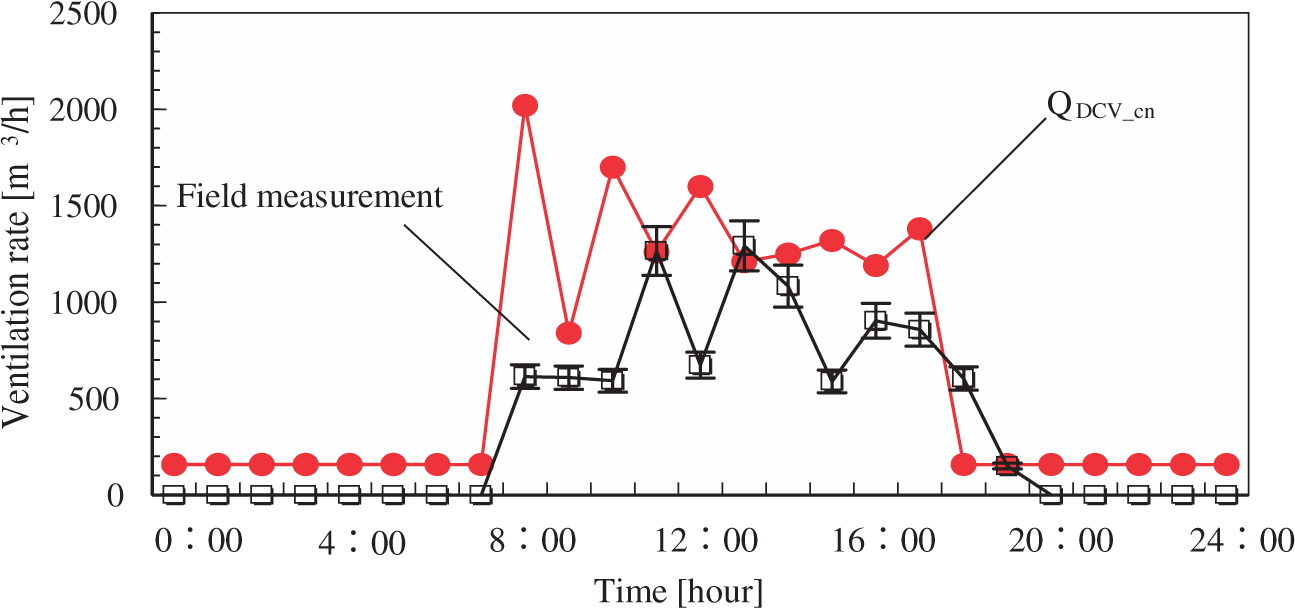
Despite these differences, the trend of the time series of the varying ventilation rate in the BES-CFD integrated simulation was in agreement with the field measurement data relatively, as shown in Figure 14. The difference was caused by inconsistent boundary conditions and the CO₂ control approach or process between simulation and testing. Relatively large fluctuations of the CO₂ concentration in the occupied zone were confirmed from 8:00 AM (the start of the workday) to 12:00 (noon), owing to the rapid increase in CO₂ generation at 8:00 AM and undesirable 1-h time-step, which was caused by default 1-h interval weather data of meteonorm in the TRNSYS, the time schedule of the occupants and a one-time-step (1 h) delay of ventilation efficiency E to optimize the ventilation rate accordingly. Thus, this overestimated concentration raises the ventilation rate to form the first and highest peak at 8:00 AM. After 3–4 mutual adjustments between BES and CFD to offset the uncertainty in each other, the prediction results for the ventilation rate became constant and displayed a trend similar to that in the results of the field measurements.

We identify this delay as being a problem with the relatively longer time intervals applied in the BES-CFD integrated simulation. In other words, this oscillation could be shortened to achieve a steady equilibrium by reducing the BES time intervals.

Carbon dioxide concentration

Figure 15 shows a time series of the CO₂ concentration of the occupied zone that was estimated by the integrated BES-CFD and CO₂ DCV simulation in accordance with the occupants pattern (see Figure 3) and testing result from the sensor which was positioned at a height of 1.5 m in the centre of the office space. The prediction results obtained from the integrated BES-CFD and CO₂ DCV simulation are approximately consistent with those of the field measurements. The occupant densities were produced from the investigation by counting the number of persons inside the field site and producing hourly average data for the input boundary condition of the numerical simulation. To clarify an appropriate representative position, the occupied zone’s average concentration that was selected for the analytical model approximately corresponds to the values of the testing sensor positioned at the centre of the office space. In addition, the return air is considered to be mixing perfectly with the room’s CO₂ level, and to also be sufficiently representative of the comprehensive effect of the indoor environment. Consequently, the difference between both the average occupied zone concentration and the average return air concentration versus the measurement results is shown in Figure 15.

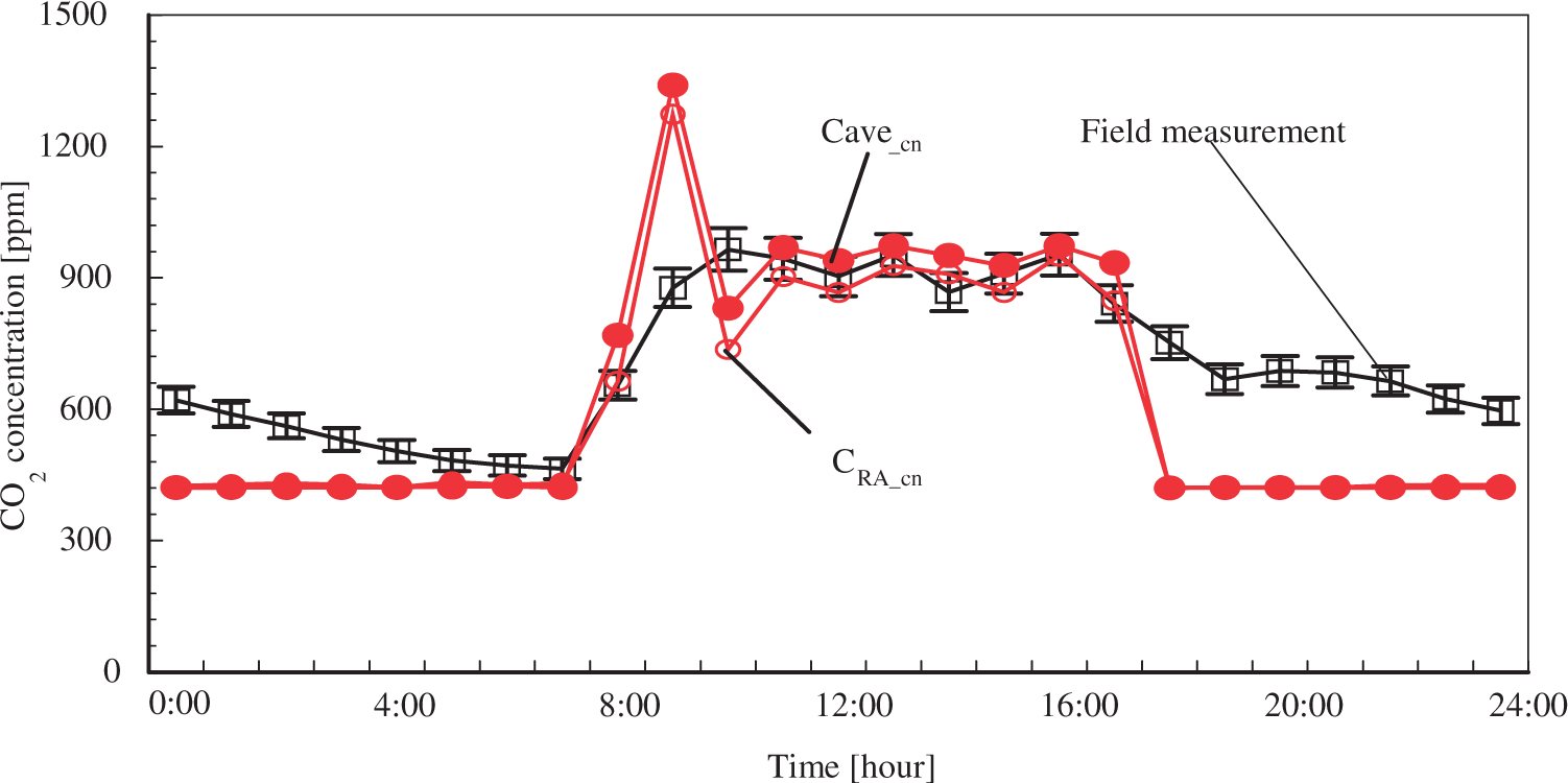
The difference between the CO₂ concentration of the average return air concentration and the average occupied zone concentration indicate that non-uniform and imperfect mixing conditions of the airflow and contaminant diffusion were created in the office space. Subsequently, the reproducibility of this non-uniform distribution in the office space by means of CFD is valid for estimating the local airflow property information. Apart from human breathing and body movement and the infiltration through building enclosure constructions, the airflow presents a proportional relationship between the occupied zone and the entire space, which is dominated by vertical thermal convection and high level of radiation between the wall surfaces with heat sources, that is, sensitive heat from human beings and electrical devices on desks, and the heat flux from lighting devices on the ceiling. In this simulation, the CO₂ level remained constant as the outdoor concentration (420 ppm_v) during night owing to the operation of the minimum ventilation rate. Because of a quasi-static boundary condition, the exchanging, lingering, and tailing dynamics of the CO₂ concentration level were not taken into account as the time-delay in the change of CO₂ concentration in the next BES time interval. However, owing to the air-tight enclosure construction without ventilation operation in the actual test site during the night, the sensor’s CO₂ concentration gradually decreased with a time-delay proportional to the order of the nominal time constant, as shown in Figure 15.

Conclusion

BES-CFD integrated simulations were able to provide detailed and informative prediction results for the heat and mass transfer in an indoor environment, and energy consumption. The prediction results with respect to energy cost saving, as well as the local airflow patterns and non-uniform distribution of CO₂ concentration, were reasonably sufficient to represent an increase in accuracy obtained by integrating the BES and CFD simulations. With the DCV module, and using the CO₂ concentration as the contamination indicator indoors, the ventilation rate could be adjusted according to the average contaminant concentration in a local target zone. Adjustment of the outdoor intake ventilation rate is considered to reduce the energy consumption while maintaining an acceptable indoor air quality through an optimized ventilation system. In this study, to control and optimize the CO₂ concentration level in the occupied zone around workers by delivering fresh supply air from the floor level, the simulation results showed a significant energy saving effect (a reduction in the outdoor air load in summer condition) for under-floor ventilation, as compared with the traditional mixing type of ventilation system with ceiling supply openings. However, owing to the limitation with 1-h time-step, which was caused by default 1-h interval weather data of meteonorm in the TRNSYS, unrealistic fluctuation existed in the first 2–3 h of the integrated simulation. More precisely, Japanese weather expansion data might be applied to the simulation in future work.

In our future study, adaptive thermal comfort theory with DCV system might be demonstrated into this integration simulation, thereby, occupied zone environment can be humanized and controlled in terms of temperature, velocity, and contaminant concentration without sacrificing more energy consumption.

Footnotes

Acknowledgement

This research was partly supported by a Grant-in-Aid for Scientific Research (JSPS KAKENHI for Young Scientists (S), 21676005). The authors would like to express special thanks to this funding source.

Appendix 1

References

Fisk

Black

Brunner

. Changing ventilation rates in U.S. offices: Implications for health, work performance, energy, and associated economics. Building Environ 2012; 47: 368–372.

Seppänen

Fisk

Mendell

. Association of ventilation rates and CO₂ concentrations with health and other responses in commercial and institutional buildings. Indoor Air 1999; 9: 226–252.

Seppänen

Fisk

Lei

. Ventilation and performance in office work. Indoor Air 2006; 16: 28–36.

Fisk

Mirer

Mendell

. Quantitative relationship of sick building syndrome symptoms with ventilation rates. Indoor Air 2009; 19: 159–165.

Lim

Schaefer

Kim

. Energy benefit of the underfloor air distribution system for reducing air-conditioning and heating loads in buildings. Indoor Built Environ 2012; 21(1): 62–70.

Zhou

Kim

. Numerical Investigation of Indoor CO₂ Concentration Distribution in an Apartment. Indoor Built Environ 2011; 20(1): 91–100.

Persily

. Evaluating building IAQ and ventilation with indoor carbon dioxide. ASHRAE Trans 1997; 103: 4072–4084.

Schell

Turner

Shim

. Application of CO₂-based demand-controlled ventilation using ASHRAE Standard 62: optimizing energy use and ventilation. ASHRAE Trans 1998; 104: 1213–1225.

ASHRAE. Standard 62.1-2007. Ventilation for acceptable indoor air quality – user's manual, Atlanta, GA: American Society of Heating, Refrigerating and Air-Conditioning Engineers (ASHRAE), 2007.

10.

O’Neill

Crawford

. Identification of flow and volume parameters in multi-zone systems using a single-gas tracer technique. ASHRAE Trans 1991; 97(1): 49–54.

11.

Ogasawara

Taniguchi

Sukehira

. Effect of energy conservation by controlled ventilation: case study in a department store. Energy Building 1979; 2: 3–8.

12.

Emmerich

Persily

. Literature review on CO₂ based demand controlled ventilation. ASHRAE Trans 1997; 103(2): 229–243.

13.

Emmerich SJ and Persily AK. State-of-the-art review of CO₂ demand-controlled ventilation technology and application. National Institute of Standards Technical Report NISTIR 6729. Department of Commerce, Gaithersburg, MD, USA, July 2001.

14.

Gan

Awbi

. Numerical simulation of the indoor environment. Building Environ 1994; 29: 449–459.

15.

Nielsen

. Velocity distribution in a room ventilated by displacement ventilation and wall-mounted air terminal devices. Energy Building 2000; 31: 179–187.

16.

Negro

COR

. Integration of computational fluid dynamic with building thermal and mess flow simulation. Building Environ 1998; 27: 155–165.

17.

Clarke

Cockroft

Conner

Hand

Kelly

Moore

O’Brien

Strachan

. Simulation-assisted control in building energy management systems. Energy Building 2002; 34(9): 933–940.

18.

Clarke

Conner

Fujii

Geros

Johannesson

Johnstone

Karatasou

Kim

Santamouris

Strachan

. The role of simulation in support of Internet-based energy services. Energy Building 2004; 36(8): 837–846.

19.

Zhai

Matzger

. Taguchi-method-based CFD study and optimisation of personalised ventilation systems. Indoor Built Environ 2012; 21(5): 690–702.

20.

Zhai

. Application of computational fluid dynamics in building design: aspects and trends. Indoor Built Environ 2006; 15(4): 305–313.

21.

Kobayashi

Chen

. Floor-supply displacement ventilation in a small office. Indoor Built Environ 2003; 12(4): 281–291.

22.

Chow

Wong

. Equations for a ventilation design derived from computational fluid dynamics. Indoor Built Environ 1998; 7: 276–288.

23.

Zhai

Chen

Haves

Klems

. On approaches to couple energy simulation and computational fluid dynamic programs. Building Environ 2002; 37: 857–864.

24.

Zhai

Chen

. Sensitivity analysis and application guides for integrated building energy and CFD simulation. Energy Building 2006; 38: 1060–1068.

25.

Djunaedy

Hensen

JLM

Loomans

MGLC

. External coupling between CFD and energy simulation: implementation and validation. ASHRAE Trans 2005; 111(1): 612–624.

26.

Fan

Ito

. Energy consumption analysis intended for real office space with energy recovery ventilator by integrating BES and CFD approaches. Building Environ 2012; 52: 57–67.

27.

Gist of the Kyoto Protocol Target Achievement Plan. Japanese environmental policy. Ministry of the Environment of Japan, http://www.env.go.jp/en/(2005, accessed 20 May 2013) http://www.env.go.jp/en/press/2005/0427b-01.pdf (accessed 20 May 2013).

28.

Takao S and Masaki T. Trends in the Japanese building ventilation market and drivers for change. Ventilation information. AIVC conference proceeding. Kyoto, Japan. 2008; 5: 25. http://www.aivc.org/medias/pdf/Free_VIPs/VIP25_Japan.pdf (accessed 20 May 2013).

29.

Bas E. Indoor air quality: guide for facility managers. USEPA, Washington D.C.: Fairmont Press, 2004, USA.

30.

Lawrence

Braun

. Evaluation of simplifies models for predicting CO₂ concentrations in small commercial buildings. Building Environ 2006; 41: 189–194.

31.

Lawrence

Braun

. A methodology for estimating occupant CO₂ source generation rates from measurements in small commercial buildings. Building Environ 2007; 42: 623–639.

32.

Sandberg

. Ventilation efficiency as a guide to design. ASHRAE Trans 1983; 89(2): 455–479.

33.

ASHRAE. Standard 129-1997 (RA2002): measuring air change effectiveness, Atlanta, GA: American Society of Heating, Refrigeration, Air-conditioning Engineers (ASHRAE), 2002.

34.

Kato

Murakami

. New ventilation efficiency scales based on spatial distribution of contaminant concentration aided by numerical simulation. ASHRAE Trans 1988; 94(2): 309–330.

35.

Mysen

Berntsen

Nafstad

Schild

. Occupancy density and benefits of demand-controlled ventilation in Norwegian primary schools. Energy Building 2005; 37: 1234–1240.

36.

Bakó-Biró

Kochhar

Clements-Croome

Awbi

Williams

. Ventilation rates in schools and pupils' performance using computerized assessment tests. Building Environ 2008; 43(4): 362–367.

37.

Nielsen

Allard

Awbi

Davidson

Schälin

. Computational fluid dynamics in ventilation design. REHVA Guidebook, Federation of European Heating and Air-conditioning Association (REHVA) Brussels, Belgium, 2007.

38.

Zhai

Zhao

Zhang

Chen

. Evaluation of various turbulence models in predicting airflow and turbulence in enclosed environment by CFD: Part-1: summary of prevalent turbulence models. HVAC&R Res 2007; 13(6): 853–870.

39.

Zhao

Zhang

Zhai

Chen

. Evaluation of various turbulence models in predicting airflow and turbulence in enclosed environments by CFD: Part-2: comparison with experimental data from literature. HVAC&R Res 2007; 13(6): 871–886.

40.

Pavlovas

. Demand controlled ventilation a case study for existing Swedish multifamily building. Energy Building 2004; 36: 1029–1034.

41.

Alalawi

Krarti

. Experimental evaluation of CO₂-based demand controlled ventilation strategies. ASHRAE Trans 2002; 108: 307–317.

Integrated building energy computational fluid dynamics simulation for estimating the energy-saving effect of energy recovery ventilator with CO 2 demand-controlled ventilation system in office space

Abstract

Keywords

Introduction

Methodology

Application to simulation

CFD model

BES model

Cases analysed

Field measurement

Results and discussion

Flow, temperature, and CO2 concentration distributions

Comparison with traditional fixed ventilation and optimized DCV

Removal efficiency of CO2 generated indoors

Time series of indoor distributions of airflow parameters

Estimation of ventilation rate and energy cost saving

Comparison between field measurement and numerical prediction

Ventilation rate prediction

Carbon dioxide concentration

Conclusion

Footnotes

Acknowledgement

Appendix 1

References

Flow, temperature, and CO₂ concentration distributions

Removal efficiency of CO₂ generated indoors