Parametric regression model for lighting calibration

Abstract

This article aims to assess some of the main lighting software programs currently available for architecture. It compares the daylight simulation results from programs, Flamingo nXt rendering, DIVA and Lightscape with the physical measurements carried out on a flat plate surface and in a model box. Identical parameters of geometry and lighting conditions were set. Two strategies were used to investigate the difference and correlation between the measurements and simulations. One test simulated several angles which were identical to the real-time sun position during daytime by rotating the box for both the simulation and field test, and the other test conducted every hour during daytime simulated three typical days (spring equinox, summer solstice and winter solstice). The output from simulation programs was conducted on a set grid of identical surface locations. The simulation programs and physical measurements were used to generate a parametric model. The results suggested that the accuracy of all these inspected simulation programs was acceptable for design exploration and that the parametric model could be used to calibrate the programs to give more accurate, real-time illuminance and luminance.

Keywords

Daylight simulation Calibration DIVA Lightscape Flamingo nXt rendering

Introduction

Appropriate architectural design, which can create delicate and ingenious daylight plays a key role in creating a comfortable visual environment while, at the same time, decreasing the energy consumption. Determination of daylight illuminance in an interior space is a key stage in daylighting studies. Simulation is an easy and flexible way for design purposes. The drive towards high lighting performance in buildings demands for more accurate and convenient operation methods to determine whether a building which relies on natural light meets the minimum standards for human visual comfort.

Recently, computer-based simulation has become increasingly important for prediction of energy and environmental performance of buildings.¹ The use of software tools for simulating lighting conditions in buildings and exterior spaces is nowadays widespread.² These building performance software give architects and engineers more confidence in building design. Studies have shown good agreements between the measured and predicted results.^3,4 Other studies found that computational lighting simulations can predict indoor illuminance more accurately than the manual methods even though the former methods have rarely been validated for real buildings with real occupancy.^5,6

In terms of daylight simulation, the sky dome is a significant determinant as the input factor. However, there is one notable shortcoming associated with many of the currently available basic lighting simulation tools: they tend to oversimplify the daylight calculations by taking only a very limited number of sky types into account.⁷ The entire set of sky types in the CIE/ISO standards is necessary in the process of daylight simulations, as oversimplification at this point of the simulation could yield significant bias.⁸ As for the lighting simulation software, architects tend to concentrate on the rendering tools.

The algorithms for producing the lighting distribution can be divided into four categories: radiosity, ray tracing, path tracing and a hybrid of these. With the advanced methods, the illuminance, glare and solar heat gain data with a focus on time variations can be clearly illustrated. Graphic outputs are created using the temporal map format to improve understanding of daylight performance as it varies by season and would enable comparisons between spatial and non-spatial quantities.⁹ In order to use the calculation technology instead of inconvenience measurement, the validation of different programs becomes a paramount task. The measurements comprise a set of ‘daylighting test cases’ that were recently developed to evaluate the simulation capabilities and limitations of different daylight simulation programs.¹ The purpose of this paper was to investigate the relationship of illuminance between lighting analysis programs and physical tests. A mathematic calibration model was established to illustrate the relationship between the predicted and measured illuminance and to provide a guideline for using simulation programs to analyse the performance of window systems. Furthermore, the accuracy of the daylight calculation was evaluated for each program.

Methodology

Sky model

The Virtual Sky Dome (VSD) approach, which divides a hemisphere into 145 patches, is one way to overcome the shortcomings of oversimplification and it has proven to be applicable to simulations with different software tools.¹⁰ The spatial luminance distribution of the sky dome is imitated by 145 distinct light sources. The distribution of the lighting sources over the hemisphere follows the conventions of sky patch luminance measurements. In particular, in 2006 it was proven that the VSD method could yield results similar to the software tools Lightscape, Radiance and that these simulations are in good accordance with measured data.¹¹

Test devices

The plate surface

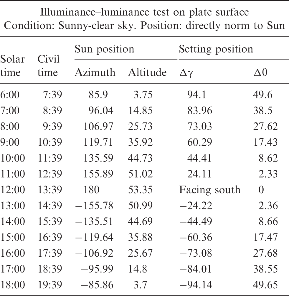
A piece of painted white wooden plate of 0.6 m × 0.4 m with a high reflectance surface was utilized to preliminarily calibrate different programs. For calibration purposes, the relationship between the illuminance and luminance for certain point on this surface was obtained. In order to obtain the highest irradiation from the sun, the tests were conducted at the solar noon. The surface could attain the largest incidence angle of solar radiation at noon time and when the plate was kept horizontal. The plate was rotated in three directions to simulate the varying sun position throughout the daytime, as shown in Figure 1. The difference of the solar angle between the solar noon and any other time on the same day was calculated and taken as the rotation increment. Taking April 4 for example, Table 1 shows the accurate angles for rotation, where the Δγ and Δθ are the rotation angles corresponding to the solar azimuth and altitude, respectively. The positive value represents the direction of upwards and clockwise, while the negative value downwards and anticlockwise. The absolute values of rotation angles were symmetrical with solar noon, 12:00. Furthermore, the CIE overcast and clear sky model was used to predict the illuminance and luminance on this surface.

Figure 1.

Tests on plate surface. (a) The plate test with tripod, (b) lighting meter, (c) angle locator.

Table 1.

The rotation angles for different time on April 4 (42°18′N, 83°42′W).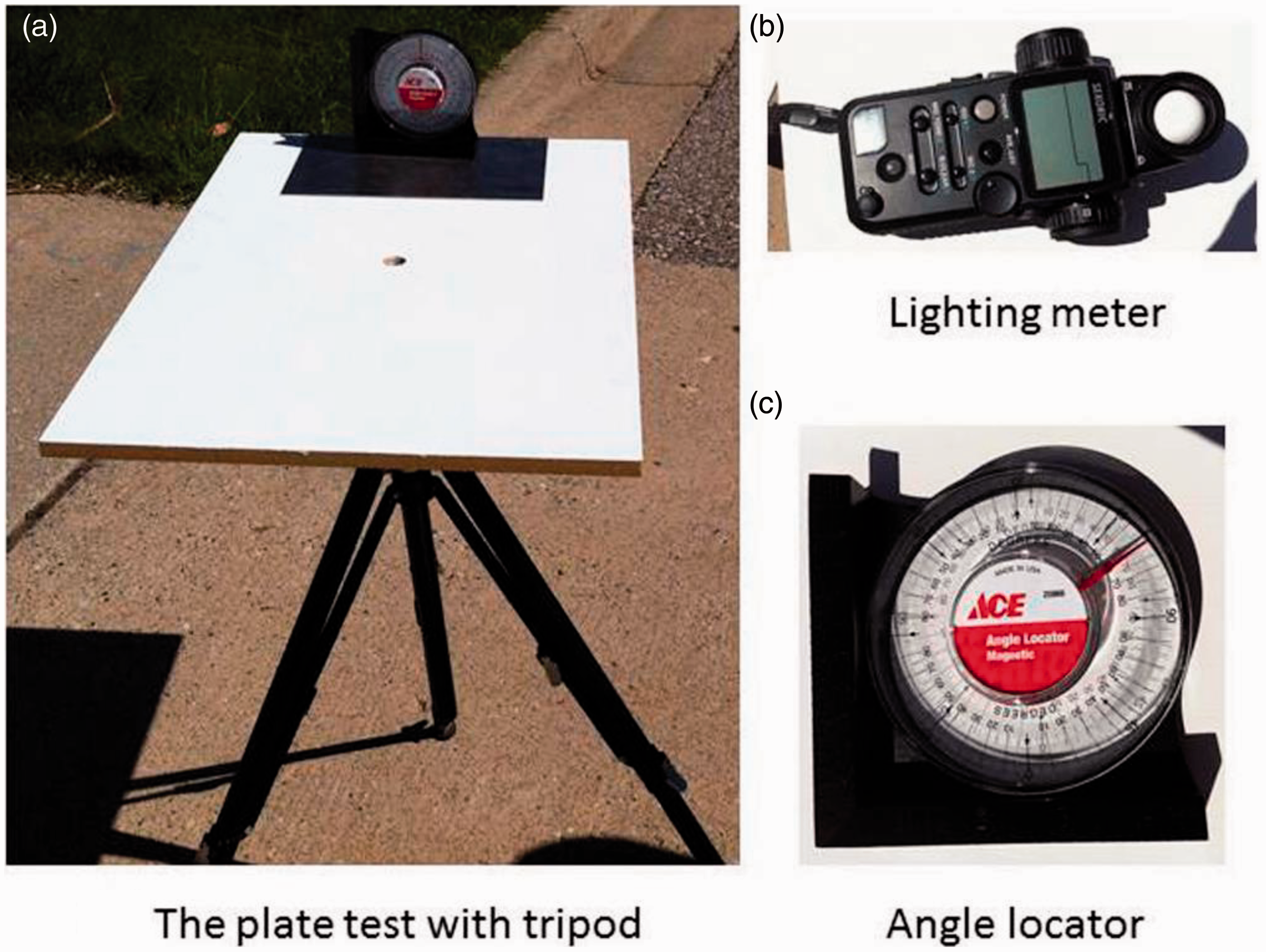

Illuminance–luminance test on plate surface Condition: Sunny-clear sky. Position: directly norm to Sun
Solar time	Civil time	Sun position		Setting position
Solar time	Civil time	Azimuth	Altitude	Δγ	Δθ
6:00	7:39	85.9	3.75	94.1	49.6
7:00	8:39	96.04	14.85	83.96	38.5
8:00	9:39	106.97	25.73	73.03	27.62
9:00	10:39	119.71	35.92	60.29	17.43
10:00	11:39	135.59	44.73	44.41	8.62
11:00	12:39	155.89	51.02	24.11	2.33
12:00	13:39	180	53.35	Facing south	0
13:00	14:39	−155.78	50.99	−24.22	2.36
14:00	15:39	−135.51	44.69	−44.49	8.66
15:00	16:39	−119.64	35.88	−60.36	17.47
16:00	17:39	−106.92	25.67	−73.08	27.68
17:00	18:39	−95.99	14.8	−84.01	38.55
18:00	19:39	−85.86	3.7	−94.14	49.65

Calibration for lighting conditions within a box

To simulate a room with natural lighting, a wooden box with the dimensions of 0.635 m ×0.381 m × 0.254 m was constructed. The box had a south-facing opening of 0.15 m × 0.15 m. The exterior surfaces were painted black to minimize the reflectance of sunlight, while five of the interior surfaces were painted white to achieve the utmost reflectiveness of sunlight inside the box. The cube can be separated into two parts, as shown in Figure 2. In the simulation programs, the black surrounding was simplified to be a black surface which was theoretically taken as a black space. The opening was at the centre of one side. In this research, there was no shading configuration installed above the opening.

Figure 2.

Schematic diagram of the box model.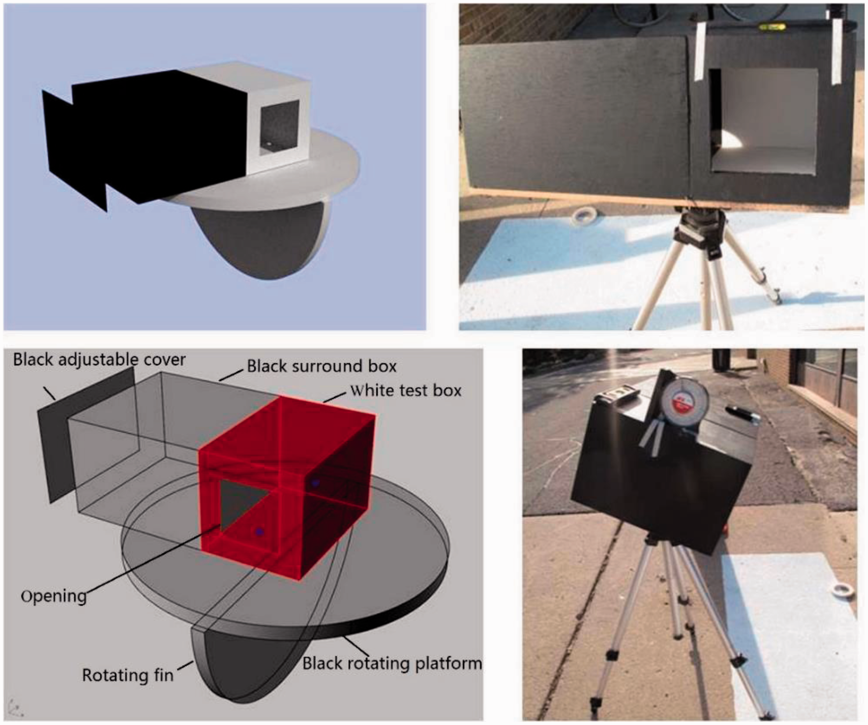

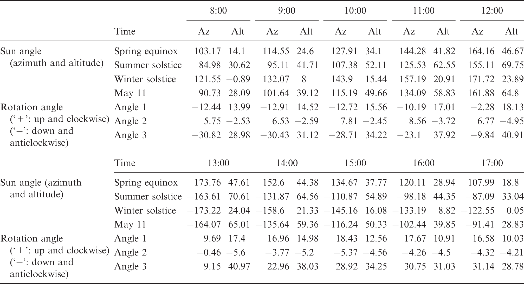
The purpose of the tests within this box was to inspect the light transmission inside the cuboid space and discover the difference between simulation and measurements that could provide further data to calibrate these programs. The solar position for three typical days (spring equinox, summer solstice and winter solstice) in a year was simulated on the test days. The daylight saving time was used and the readings were conducted hourly from 9:00 to 17:00. The difference on the solar azimuth and altitude between the simulated days and test day was taken as the rotation angles. The aim was not trying to simulate the real situation on these three days but to discover the veracity of the program predictions for different angles. Table 2 lists the solar angles for the three typical days and the rotation angles when the tests were conducted on May 11.

Table 2.

The relevant sun angle and rotation angles for three typical simulation and the test day (42°18′N, 83°42′W).

		8:00		9:00		10:00		11:00		12:00
	Time	Az	Alt	Az	Alt	Az	Alt	Az	Alt	Az	Alt
Sun angle (azimuth and altitude)	Spring equinox	103.17	14.1	114.55	24.6	127.91	34.1	144.28	41.82	164.16	46.67
	Summer solstice	84.98	30.62	95.11	41.71	107.38	52.11	125.53	62.55	155.11	69.75
	Winter solstice	121.55	−0.89	132.07	8	143.9	15.44	157.19	20.91	171.72	23.89
	May 11	90.73	28.09	101.64	39.12	115.19	49.66	134.09	58.83	161.88	64.8
Rotation angle (‘+’: up and clockwise) (‘−’: down and anticlockwise)	Angle 1	−12.44	13.99	−12.91	14.52	−12.72	15.56	−10.19	17.01	−2.28	18.13
	Angle 2	5.75	−2.53	6.53	−2.59	7.81	−2.45	8.56	−3.72	6.77	−4.95
	Angle 3	−30.82	28.98	−30.43	31.12	−28.71	34.22	−23.1	37.92	−9.84	40.91
	Time	13:00		14:00		15:00		16:00		17:00
Sun angle (azimuth and altitude)	Spring equinox	−173.76	47.61	−152.6	44.38	−134.67	37.77	−120.11	28.94	−107.99	18.8
	Summer solstice	−163.61	70.61	−131.87	64.56	−110.87	54.89	−98.18	44.35	−87.09	33.04
	Winter solstice	−173.22	24.04	−158.6	21.33	−145.16	16.08	−133.19	8.82	−122.55	0.05
	May 11	−164.07	65.01	−135.64	59.36	−116.24	50.33	−102.44	39.85	−91.41	28.83
Rotation angle (‘+’: up and clockwise) (‘−’: down and anticlockwise)	Angle 1	9.69	17.4	16.96	14.98	18.43	12.56	17.67	10.91	16.58	10.03
	Angle 2	−0.46	−5.6	−3.77	−5.2	−5.37	−4.56	−4.26	−4.5	−4.32	−4.21
	Angle 3	9.15	40.97	22.96	38.03	28.92	34.25	30.75	31.03	31.14	28.78

Simulation programs

The three programs discussed below are common in the field of building design and they use different algorithms to realize the simulation. They were selected because of their representativeness. Each of them has advantages and limitations. Therefore, none of them is 100% accurate and that is why this study attempts to find a ‘calibration factor’ which can convert the calculation results into information more useful for design purposes. The strength and weakness of these algorithms could be revealed through the analyses. When the field measurement becomes overly complicated and difficult to conduct, this factor could be used to obtain close-to-realistic lighting distribution inside the building based on values given by simulation programs. Such factor may also help to shed light on how to improve the current algorithms.

DIVA

DIVA, which stands for Design Iterate Validate Adapt, is an environmental analysis plug-in for the Rhinoceros 3D Nurbs modelling program.^12,13 The integration of iterative method was used for light transmission inside the building model. DIVA performs a daylight analysis on an existing architectural model via integration with Radiance and DAYSIM.¹⁴ The lighting simulation itself uses the ray tracing techniques,¹⁵ which are typically arranged to form a photographic quality image, to compute radiance values (i.e. the quantity of light passing through a specific point in a specific direction). The Radiance strictly works in the backward direction. The primary advantage of Radiance is that there are no limitation on the geometry or the material that might be simulated. However, computing light from some systems, such as curved specular surfaces, would require a ray tracing method that follows light in the forward direction, starting at the emitters and working outward. A separate preprocess would be necessary to compute the output distributions.

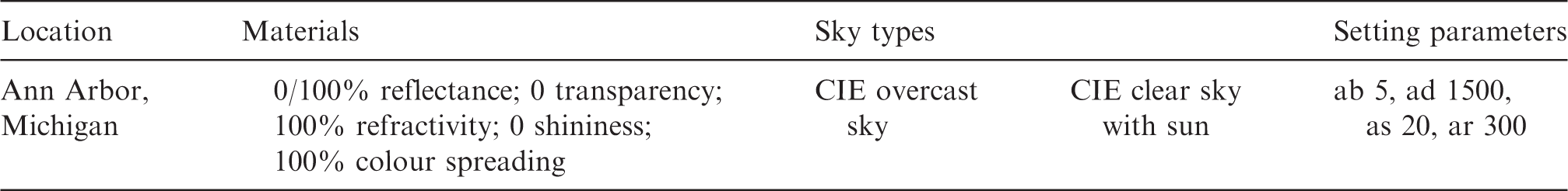
The typical meteorological year climate which utilizes one of CIE four possible sky distributions has been input for lighting calculation while defining the geographic project location. Based on the previous sky algorithm research, the CIE standard model covers the entire occurrence spectrum which comprises direct sunlight and different types of diffuse scattering by the atmosphere. By applying additional parameterization, illuminance and luminance levels can be calculated not only in relative physical units but also in absolute ones.¹⁶

The illuminance on the observed surface under certain weather condition can be predicted by mesh nodes. The user can either select the default values for different materials from the built-in library or enter new values. Furthermore, the luminance at different points can be obtained through the visualization rendering. This climate-based DAYSIM program can provide the illuminance and luminance values of the points when the editable materials from Radiance library were utilized. The simulation parameters and materials are listed in Table 3.

Table 3.

The parameters and materials of DIVA simulation.

Location	Materials	Sky types		Setting parameters
Ann Arbor, Michigan	0/100% reflectance; 0 transparency; 100% refractivity; 0 shininess; 100% colour spreading	CIE overcast sky	CIE clear sky with sun	ab 5, ad 1500, as 20, ar 300

Lightscape

As mentioned earlier, the VSD method for the sky model was used in program Lightscape to provide three-dimensional model simulations under the real-world conditions. The CIE sky model was also used in this program and sky conditions in Lightscape would be defined by the proportion of the sky covered by the clouds.

LIGHTSCAPE uses the progressive refinement Radiosity algorithm and a post-processing Ray tracing as the calculation method. Ray tracing follows all rays from the eye of the viewer back to the light sources. Radiosity simulates the diffuse propagation of light starting at the light sources. Radiosity simulates diffuse light transport in terms of visibility between surfaces, rather than taking paths from light sources to surfaces. The advantage of the ray-tracing procedure is that it works at pixel resolution and that the variance is still acceptable for the first- or second-order inter-reflections. On the other hand, the radiosity method offers a total solution, and the higher order reflection effects are obtained at a bearable cost, albeit biased by degeneration.¹⁷ Calculating the overall light propagation within a scene for global illumination is a very difficult problem. With a standard ray tracing algorithm, this is a very time-consuming task, since a huge number of rays have to be shot. For this reason, the radiosity method was invented. The main idea of the method is to store illumination values on the surfaces of the objects, as the light is propagated starting at the light sources. It only works with Lambertian surfaces, since the only thing that affects the transmission intensity is simplified to be the cosines of the angles between the light transport direction and the surface normal. The principle was the same as the Lambert's law. This hybrid approach cannot be considered an advanced method, because there is no indication that Ray Tracing participates in the calculation of the light transferred to surfaces. The numerical and tonality analyses are generated independently of the post-processing Ray Tracing. One of its main impediments concerns with the fact that the correction of programming problems will not happen due to its discontinuity. Therefore, the evolution of its algorithm is compromised beyond the problems of support to the user.¹⁸ Lightscape uses two approaches to deal with the interior and exterior daylights. When the interior daylight algorithm is used, the daylight and sunlight can be calculated only for surfaces specified as windows or openings. The lighting detail should be provided to get enough elements on the surface, for the number of mesh element required to capture the illumination of a surface depends on the complexity of the illumination on that surface.

The weighted approximate factors were adopted in this program by this study to predict the absolute values of illuminance and luminance on the surface. The virtual model, including the sky model, the location, the time and the reflectiveness of the surfaces, was identical to the model in the field test.

Flamingo nXt

This program uses the path tracing technology to produce the images of realistic results. Different from the form factor computation method used in the Lightscape which forces all surfaces to be Lambertian or ‘perfectly diffuse’. It does not exist in the real world, and the path tracing is a much more accurate method since it always includes the entire model (Global Illumination).^15,19 Instead of obtaining the light from lighting sources, this algorithm would integrate all the illuminance arriving to a single point on the surface of an object.²⁰ This illuminance is then reduced by a surface reflectance function to determine how much of it will go towards the viewpoint camera. This integration procedure is repeated for every pixel in the output image.²¹ The indirect lighting as well as complex reflection and refraction can be incorporated into the simulation. In other words, three principles should be followed:

For a given indoor scene, every object in the room must contribute illumination to every other object.

There is no distinction between illumination emitted from a light source and that reflected from a surface.

The illumination coming from surfaces must scatter in a particular direction that is some function of the incoming direction of the arriving illumination and the outgoing direction being sampled.

Unlike the radiosity, this program does not require the perfectly diffuse surfaces.¹⁹ Based on the interior and exterior daylight simulations, high dynamic rendering image-based lighting and many other techniques, the luminance of each pixel is the output from the nXt rendering. The paths could be modified easily and quickly. The main factor that makes modifications so fast is that, when the user goes through path tracing steps, the path integral of each point is known. At any given point as the user starts unrolling the recursion down a sample path, the path integral would be computed up to that point, so a variation in the path such as adding or removing or replacing a vertex would add an extra term and/or remove an existing one up to that point in the path. Furthermore, the amount and direction of light can be captured in a scene. This program was taken as the plug-in within the Rhinoceros 3D modelling software. All the input parameters of the program were consistent with the conditions of the field tests.

The surface of models built in simulation programs was assumed to be perfectly diffuse, which differed from the real physical models. This might cause some discrepancy between these two methods.

Field measurements

All of these tests were conducted at the School of Art and Architecture in University of Michigan, Ann Arbor, Michigan, USA (42°18′N, 83°42′W). The first field test was carried out with a painted white plate surface described before under the overcast and clear sky conditions to investigate the relationship between illuminance and luminance of the surface and the initial conversion of lighting results from simulation results to test readings. The second field test analysed the same relationship within the scaled physical model (the box) under the clear sky condition. In this field test, three conversion rotation angles corresponding to three typical days were simulated, respectively, spring solstice (case 1), summer equinox (case 2) and winter equinox (case 3). The adjustments of the box position were achieved by regulating the rotation angles of the tripod. The third field obtained the photo exposure values (EVs) inside the box to compare with the test values. The shading materials were introduced in this test to determine the difference and the relationship between test readings and conversion values from camera. The shading materials were set on the opening of the box and these consisted of plastic plates with different light transmittance, the aerogel plate and paper plates with different aperture. The information of even plastic plates were listed in Table 4.

Table 4.

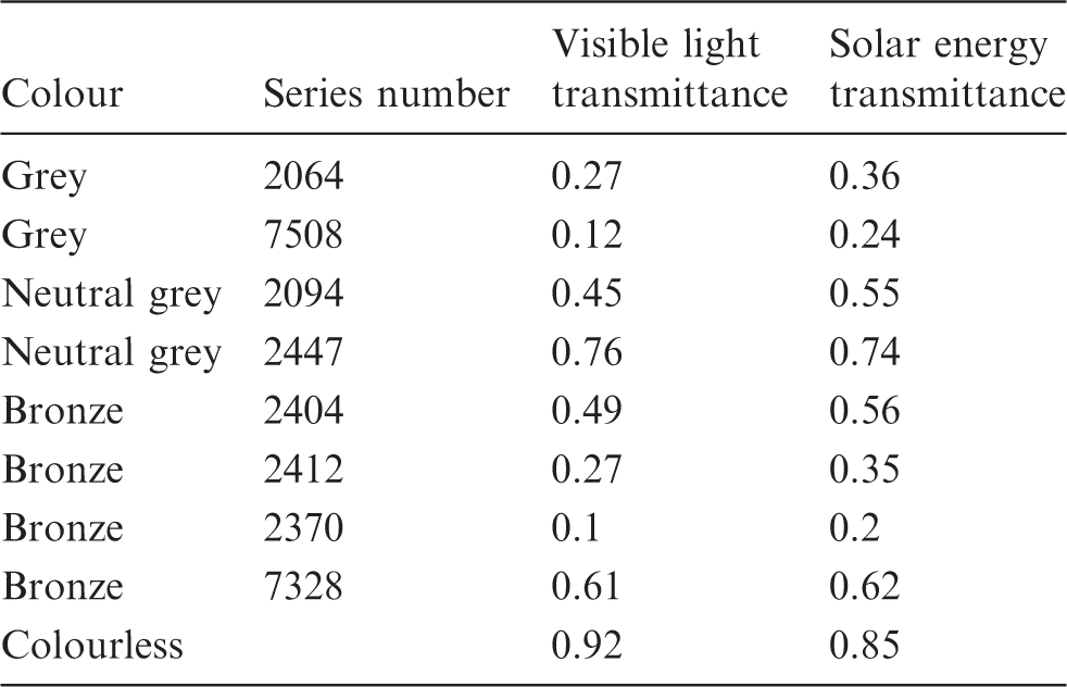
Parameters of different shading materials.

Colour	Series number	Visible light transmittance	Solar energy transmittance
Grey	2064	0.27	0.36
Grey	7508	0.12	0.24
Neutral grey	2094	0.45	0.55
Neutral grey	2447	0.76	0.74
Bronze	2404	0.49	0.56
Bronze	2412	0.27	0.35
Bronze	2370	0.1	0.2
Bronze	7328	0.61	0.62
Colourless		0.92	0.85

The lighting meter, Sekonic L-758C, with the accuracy of ±1 lux, ±1 cd/m², shown in Figure 1, was used to record the illuminance and luminance at the point on the surface as well as inside the box. This light meter was recalibrated by an illuminometer which recorded the illuminance of one certain point besides the office building for 24 h. The precision was 0.5 lux and 0.5 cd/m². The photos were taken by a camera using the settings with ‘Aperture’ equal to f/4 and ‘Time of Exposure’ equal to 1/250 s. The test point inside the box is shown in Figure 3. The luminance of tested point was read directly by setting lighting meters on a certain point, but the illuminance was obtained by shooting on this certain point from a distance of 60 cm. For the plate surface test, the lighting meter and the angle locator were fixed on the surface by hand. For the tests within the box, both the lighting meter and camera were located in the middle of the surface which was on the opposite side of the test surface. There was a hole with a diameter of 3 cm, at which, the sensor of lighting meter and the camera lens could be inserted. The angle locator was set on the top surface of the box.

Figure 3.

Diagram of the model and test point.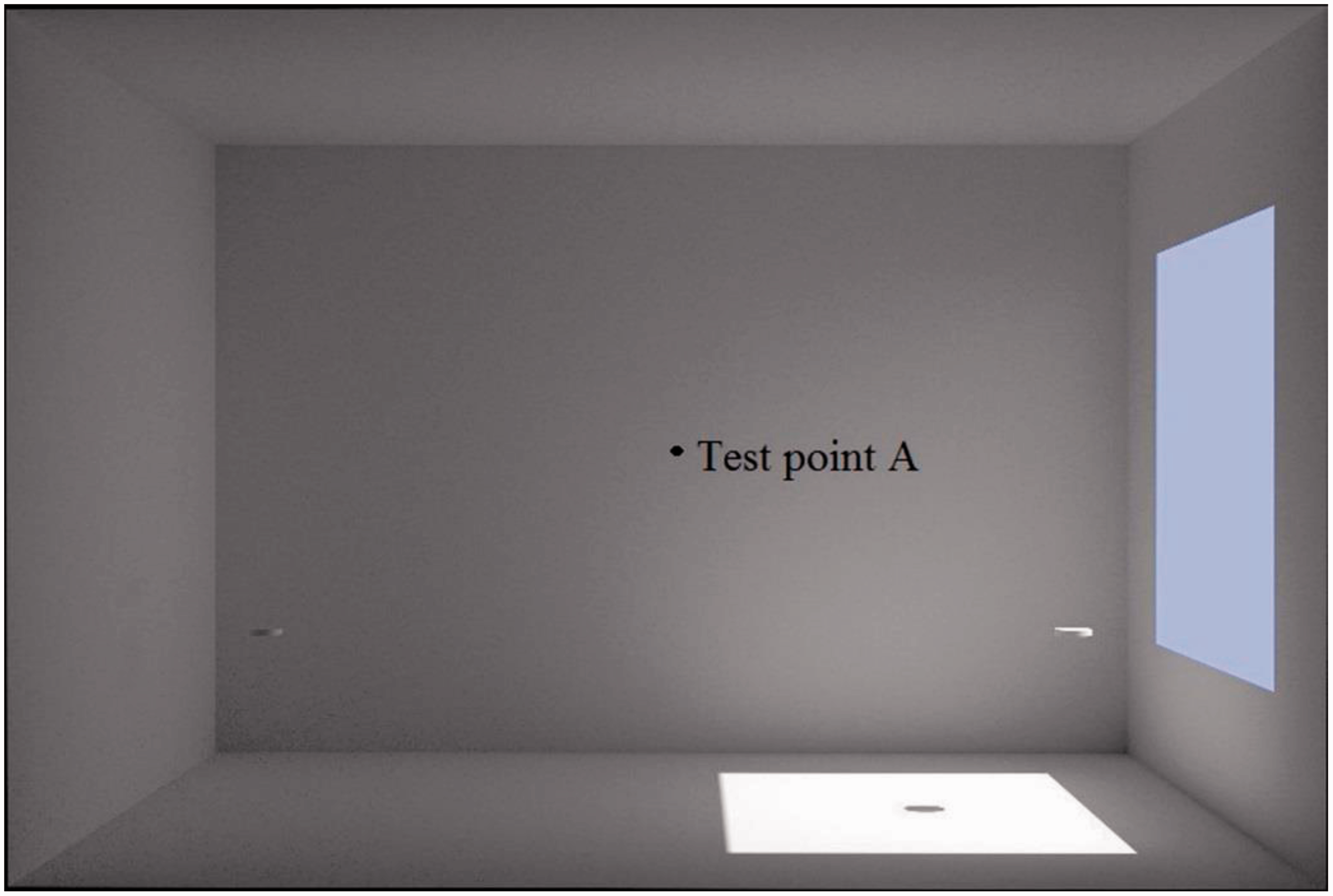

The dial gauge for azimuth and tilt angles of the tripod was the guide to adjust the position of the model. The accuracy of the reading was 0.1°. The crabstick with a length of 0.1 m was placed perpendicular onto the material surface to check the position of the model. The shadow of this crabstick was the criteria used to adjust the model. In advance, the projection lines starting from the same point with length and direction calculated according to different sun position were marked on a blank paper. At the same time the orientation was also confirmed on this paper. The crabstick and this paper were both stuck on the horizontal surface of the models. When the shadow of this crabstick was coincided with the corresponding line on the paper, this would therefore represent the model being at the right position.

Data analysis method

Readings were repeated three times in every test and the mean value of them was obtained and taken as the final results. Outlier analysis was made firstly to remove exceptional values from the obtained results. A range between 25th–1.5IQR and 75th+1.5IQR (inter quartile range (IQR)) was used as the non-outlier range.²² Data collected in the tables (with removed outliers) were then summarized with descriptive statistics. A confidence level of 95% represents statistically significant coefficients. The coefficient of determination (R²) shows the accuracy of the regression model.

Results

All the results from simulation programs and tests were obtained under clear and overcast sky. Simulation packages DIVA and Lightscape allow the user to enter two sky conditions: clear and overcast sky. In simulation package Flamingo nXt, however the user sets the sky condition by adjusting the sun and sky button between 0% and 100%. The reflectivity and refractivity of all the materials were 1.0 in all simulations. The location for daylight analysis was set to 42°N, 83°W.

Light availability on the plate surface

Clear sky

Tests under the clear sky condition were conducted on sunny days. The illuminance and luminance of the surface were recorded. Take the case on April 6 for example, seen from Figure 4, the luminance values from three programs (Flamingo rendering, Lightscape and DIVA) and test readings were displayed, but the illuminance values were from Lightscape, DIVA and test readings, because the Flamingo nXt rendering could only provide the luminance values. The illuminance values at noon time output from Lightscape and test was setup to 90,000lux or more when the plate was kept at the original place. The difference was less than 5%. However, with increased rotation angles, the difference became significant, up to 74%. Results from DIVA were shown to deviate from the test readings with the small rotation angles in comparison to the bigger ones. The largest difference between the measured and simulated illuminances was 30%; about 20,000 lux as the difference between the results of DIVA and Lightscape. The tendency of luminance distribution on the surface is similar to that of the illuminance for these simulation and test.

Figure 4.

Lighting availability on the plate surface.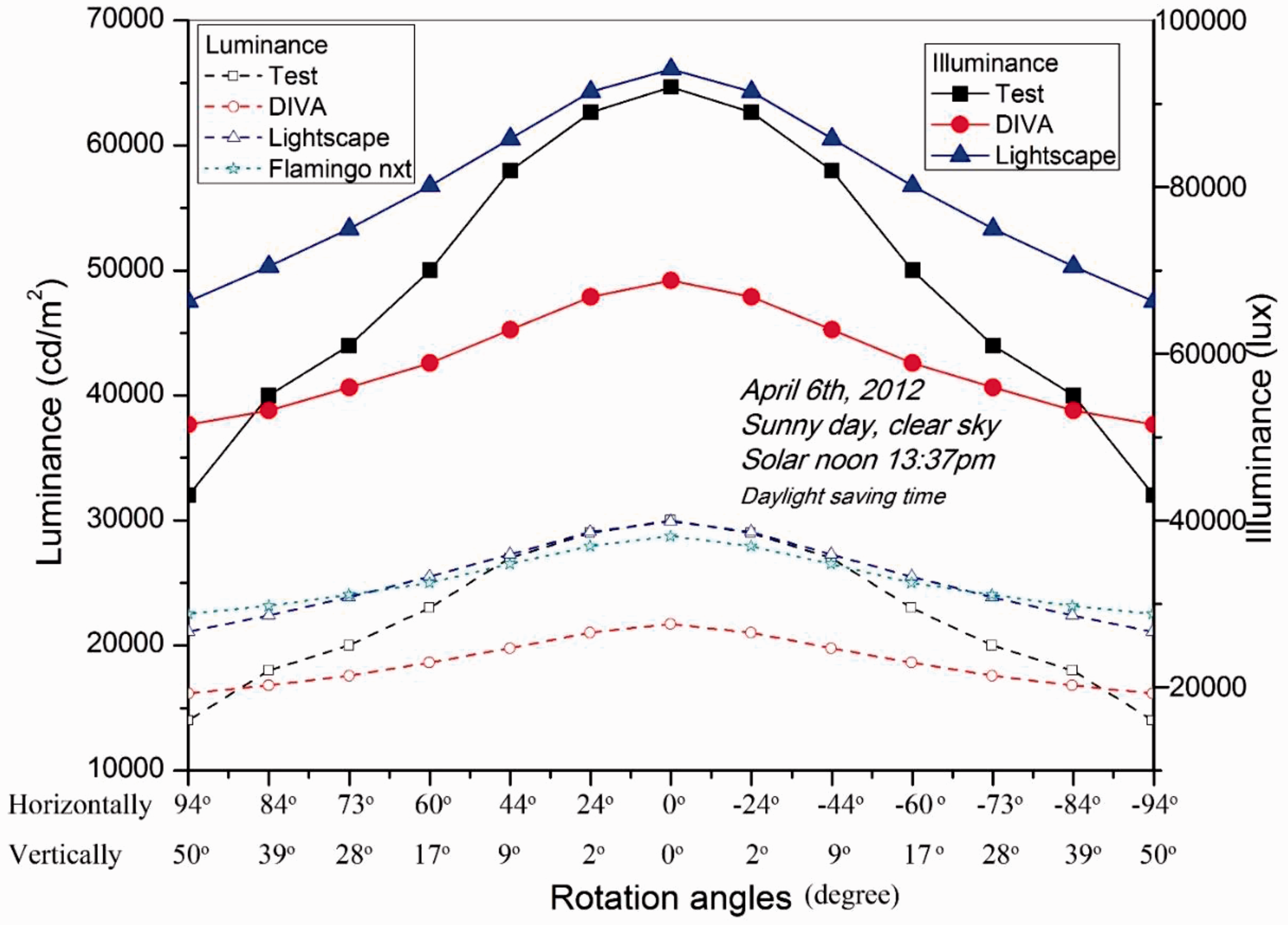

We found that programs nXt and Lightscape gave similar results. For all these simulations except the DIVA, less accurate luminance values at higher rotation angles than that on the origin point where the rotation angles were 0 were predicted. When the solar angle deviated more from the North–South axis, the measured luminance was lower than that given by the calculation. It is obvious that the simulations had overestimated the luminance and illuminance values at higher rotation angles.

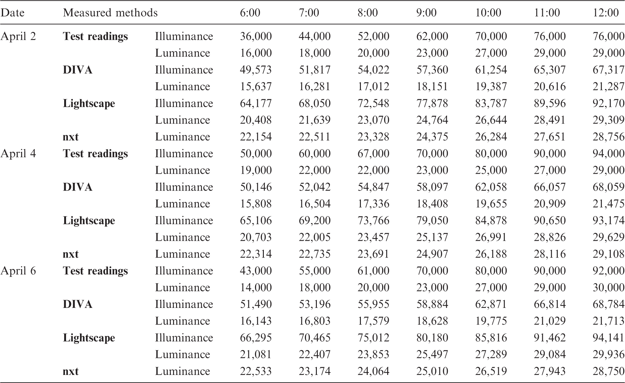
In order to investigate the relationship between illuminance and luminance for a given surface, it is necessary to establish correlations between the two variables. The measured data for the 2 April, 4 April and 6 April 2012 were presented in Table 5. Figure 5 represents the mathematical parametric model for programs showing the π linear function as the relationship between illuminance and luminance, providing the fitting curve for DIVA and Lightscape.²³ The difference between them was that this conversion factor was taken as the input parameter and can be considered as the weighted approximates of the Lightscape. By this way, the illuminance values were determined as soon as the luminance output. However, the luminance values were recorded from DIVA rendering based on the ray tracing algorithm, meanwhile the illuminance values and lighting distribution were printed on the nodes. From test readings, the conversion factor between illuminance and luminance was 3.1, which was a little lower than the simulations, with the R² equal to 0.95, giving the linear fit with the intercept being zero.

Figure 5.

Relationship between illuminance and luminance from tests and simulations.

Table 5.

The results from simulation programs and tests on 2 April, 4 April and 6 April 2012.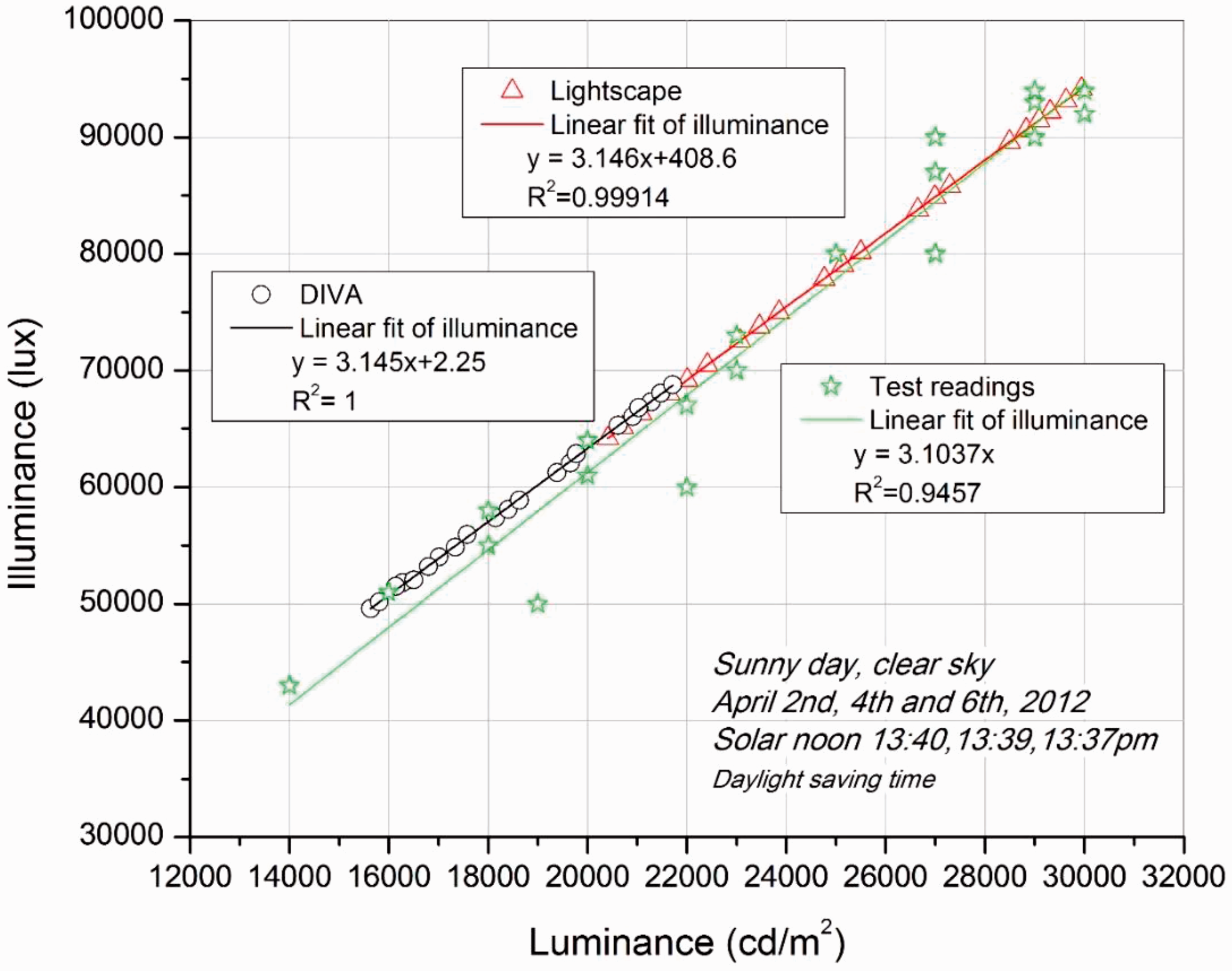

Date	Measured methods		6:00	7:00	8:00	9:00	10:00	11:00	12:00
April 2	Test readings	Illuminance	36,000	44,000	52,000	62,000	70,000	76,000	76,000
	Test readings	Luminance	16,000	18,000	20,000	23,000	27,000	29,000	29,000
	DIVA	Illuminance	49,573	51,817	54,022	57,360	61,254	65,307	67,317
	DIVA	Luminance	15,637	16,281	17,012	18,151	19,387	20,616	21,287
	Lightscape	Illuminance	64,177	68,050	72,548	77,878	83,787	89,596	92,170
	Lightscape	Luminance	20,408	21,639	23,070	24,764	26,644	28,491	29,309
	nxt	Luminance	22,154	22,511	23,328	24,375	26,284	27,651	28,756
April 4	Test readings	Illuminance	50,000	60,000	67,000	70,000	80,000	90,000	94,000
	Test readings	Luminance	19,000	22,000	22,000	23,000	25,000	27,000	29,000
	DIVA	Illuminance	50,146	52,042	54,847	58,097	62,058	66,057	68,059
	DIVA	Luminance	15,808	16,504	17,336	18,408	19,655	20,909	21,475
	Lightscape	Illuminance	65,106	69,200	73,766	79,050	84,878	90,650	93,174
	Lightscape	Luminance	20,703	22,005	23,457	25,137	26,991	28,826	29,629
	nxt	Luminance	22,314	22,735	23,691	24,907	26,188	28,116	29,108
April 6	Test readings	Illuminance	43,000	55,000	61,000	70,000	80,000	90,000	92,000
	Test readings	Luminance	14,000	18,000	20,000	23,000	27,000	29,000	30,000
	DIVA	Illuminance	51,490	53,196	55,955	58,884	62,871	66,814	68,784
	DIVA	Luminance	16,143	16,803	17,579	18,628	19,775	21,029	21,713
	Lightscape	Illuminance	66,295	70,465	75,012	80,180	85,816	91,462	94,141
	Lightscape	Luminance	21,081	22,407	23,853	25,497	27,289	29,084	29,936
	nxt	Luminance	22,533	23,174	24,064	25,010	26,519	27,943	28,750

The luminance values were taken as the primary data to investigate the relationship between the simulation programs and the field measurements, on the basis of the parametric model. The polynomial fit clearly manifests the optimal conversion relationship with the R² value up to 0.92, as shown in Figure 6. These examples suggest that the designers should take caution when selecting appropriate simulation programs.

Figure 6.

Correction factor with test readings for different programs.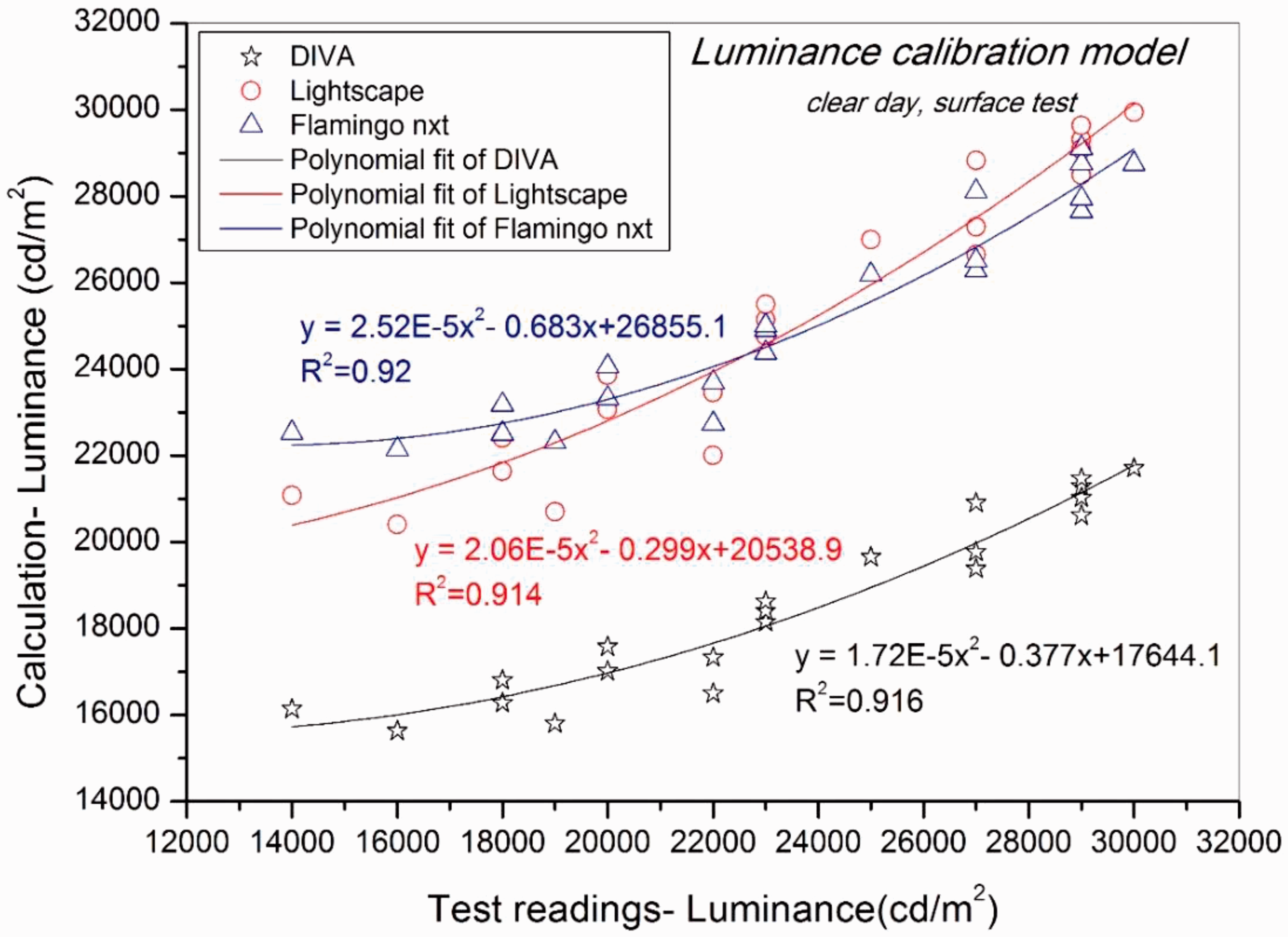

Overcast sky

The illuminance and luminance of the surface under cloudy sky condition were illustrated in Figure 7. A few notes need to be stated about these tests. On the test day, March 29, data were recorded from several cloudy days because the sky condition was most close to overcast sky. The thickness of the clouds could not be measured, so we choose the test day when the sky was covered with the most uniform, thick clouds. Furthermore, the property of the sky for simulation was according to CIE overcast sky.²⁴ For the rendering in Flamingo nXt, the luminance of the surface under the overcast sky condition was obtained by turning off the channel of sunlight and leaving the daylight channel on.

Figure 7.

Measured and simulated illuminance and luminance under overcast condition.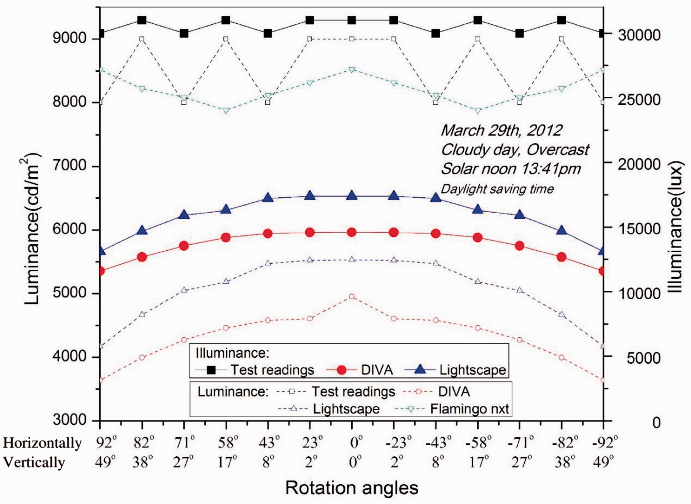

The measured illuminance was up to 30,000 lux, which was almost twice as much as the results from DIVA and Lightscape simulations. Due to the same settings used in these two programs, similar results on the magnitude as well as the tendency were obtained, though the Lightscape gave higher values. The luminance of the surface predicted by the Flamingo nXt rendering were the closest to the tests with a variation from 8000 to 9000 cd/m², while the results from the other two simulation results varied between 3500 and 5500 cd/m². The difference of illuminance and luminance could be recognized more easily under the overcast condition than under the clear sky condition.

Lighting distribution inside the box

The calibration models obtained from the surface tests were applied to box tests to measure the illuminance in the box because of the confined interior space and the need to obtain the illuminance readings manually. The results from the Flamingo nXt rendering utilized the same method to calculate the illuminance values based on the luminance readings obtained by the manual test. These shortcomings disappeared for simulation in DIVA and Lightscape, with which the illuminance and luminance could be obtained at the same time.

The output screens of the three programs are shown in Figure 8. All the programs display the readings by clicking the relevant point. Obviously the Flamingo nXt rendering would give the clearest image which reflects the most realistic condition.

Figure 8.

Output interface from different programs. (a) The calculated luminance from Lightscape, (b) the rendering graphic from Flamingo nXt, (c) the calculated illuminance from DIVA.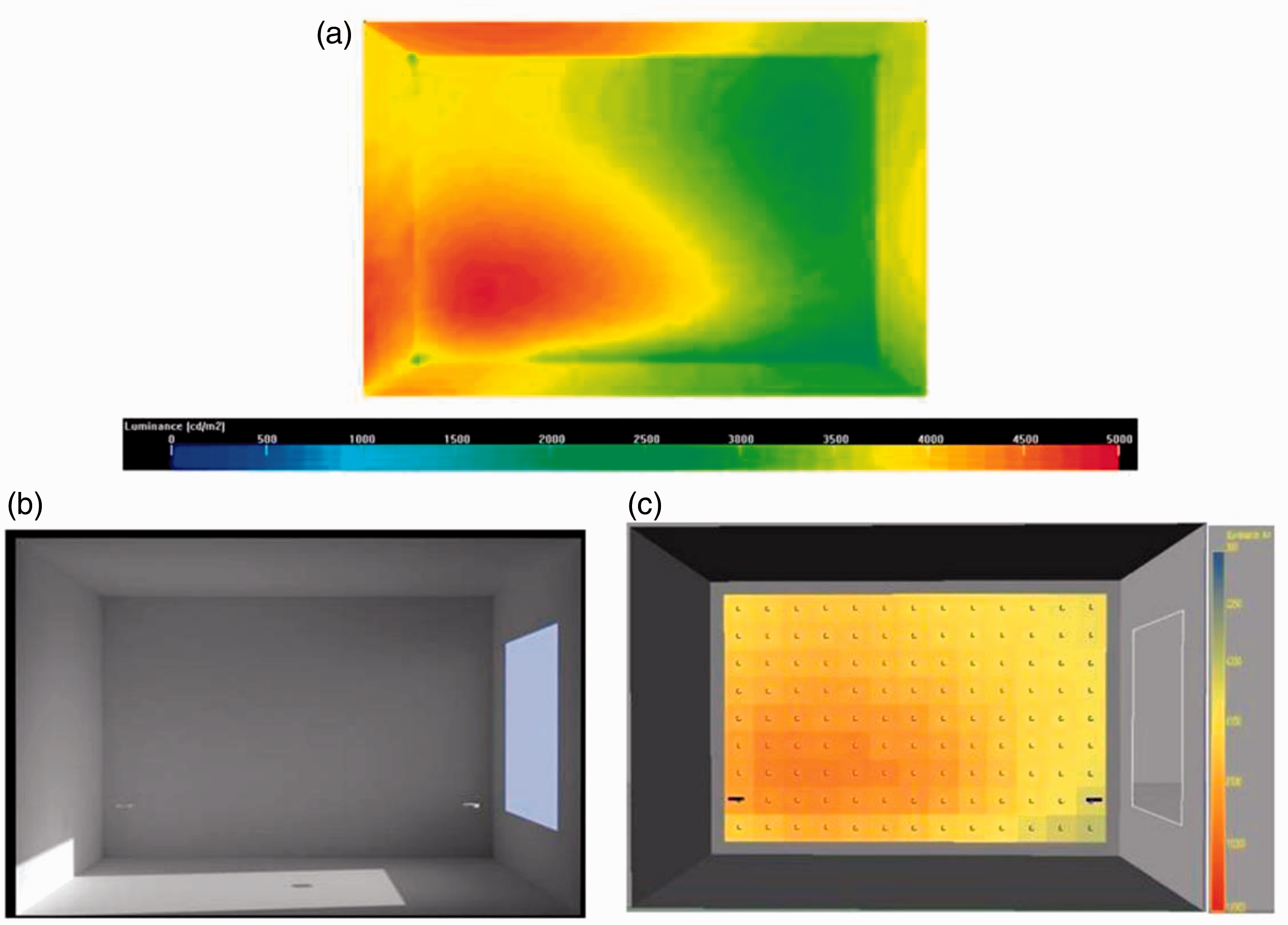

The illuminance and luminance distribution in the box

Figure 9 depicts the measured and simulated illuminance and luminance for three sets of rotation angles. It can be seen that the illuminations (illuminance and luminance) inside the box differed substantially for the three sets of angles. Angle setting 3, which is the biggest rotation angle, resulted in the highest light transmission. The illuminance and luminance recorded for angle setting 2 with the highest relative altitude angle of the sun were below, respectively, 5000 lux and 2000 cd/m², which were more significant than the other two cases. The largest difference was 68.2%. This would make sense because the tests were carried out in May, so the smallest rotation angle would represent the situation in summer when the solar angle was high and the light transmission to the box was less than that in winter.

Figure 9.

Lighting performance on test point for different angles.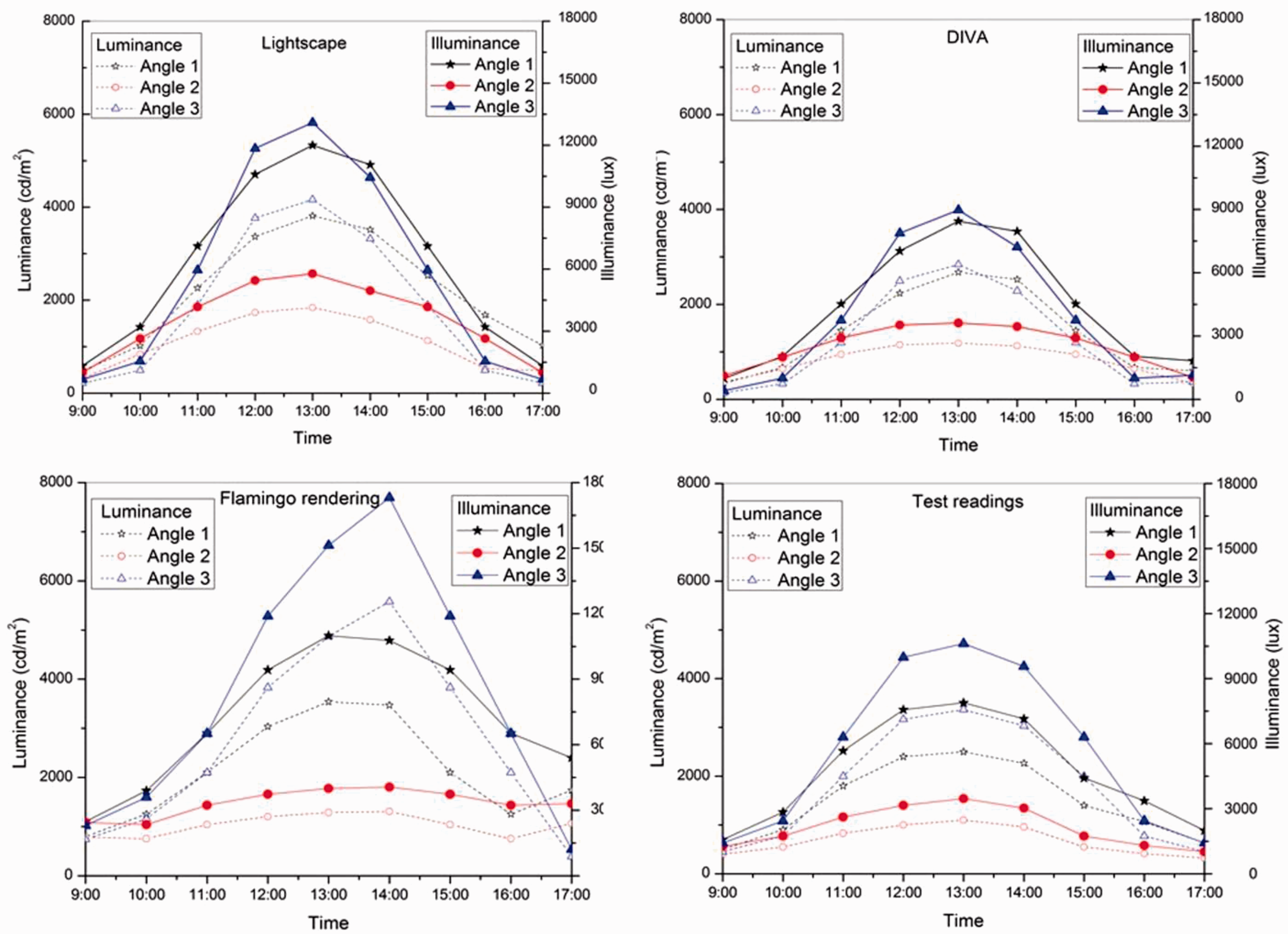

The values obtained from this field test were lower than the ones given by any simulation program, especially the Flamingo nXt rendering and Lightscape. The difference of 40% and 61.7% in illuminance values from Lightscape and tests was, respectively, found for case 2 and case 3. This was different from the results of surface tests, due to the different settings of physical texture, which could cause some variances on the lighting transmission. Therefore, the choice of physical model used in the simulation program should be considered carefully.

Compare readings from photo exposure and tests

The view inside the test box was recorded by the camera, as seen in Figure 10. These photos were taken at 15:00 on June 27. The shading panels were changed one by one as fast as possible. The ISO setting of the camera was 100. The luminance values would be obtained from light level chart by searching for the exposure times (s), f-number and the EVs. For example, the f-number of 4 and the exposure time of 1/160 s were selected when inspecting the shading material of the grid. The EV would be determined to be 12.5 by these two parameters. The luminance under the condition of ISO 100, K = 12.5 would be 400 cd/m². All the other luminance values would be estimated this way. These values were the average readings for a whole surface, so big difference would be obtained when compared with the test readings.

Figure 10.

View inside the box with different shading configurations. ‘M’ stands for the material covering the opening. ‘LV’ stands for the luminance value inside the box. The outside horizontal illuminance value was 80,000 lux.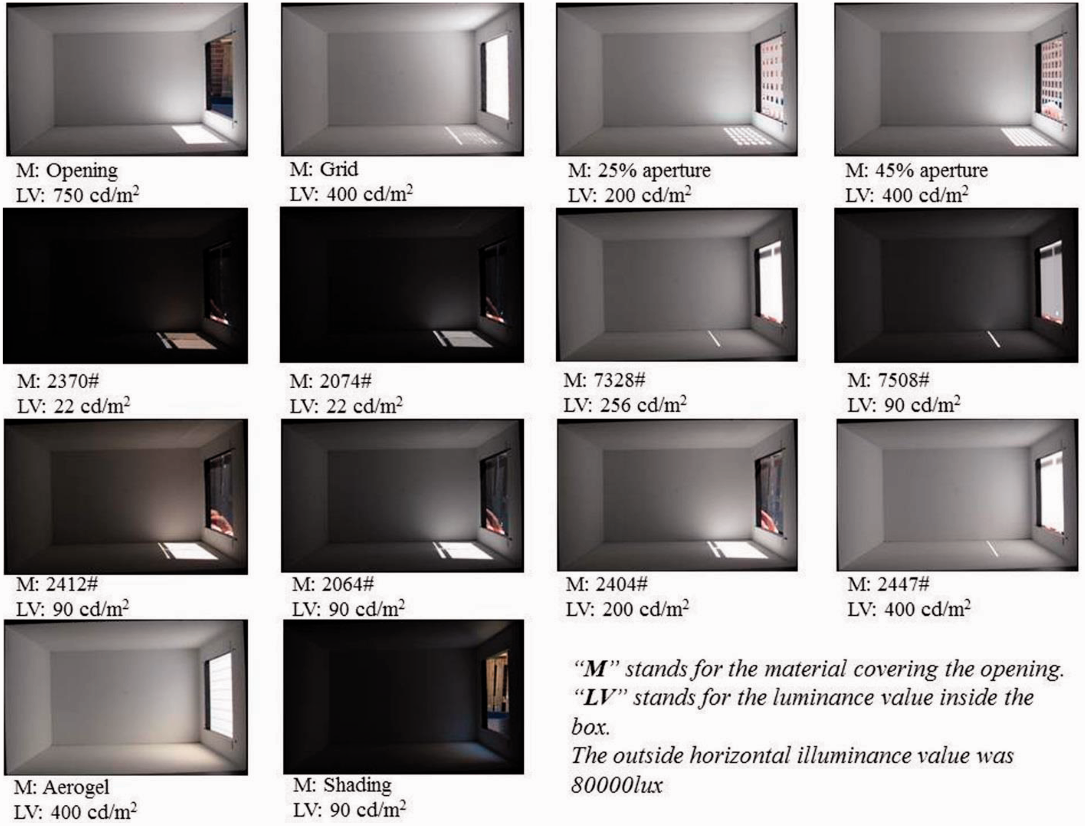

Figure 11 illustrates the relationship between these two kinds of results. The values obtained from the photo exposure were much lower than those from measurements. The latter ones were almost 1.65 times more than the former ones. On the other hand, the results also illustrate the need of a correct factor between the photo exposure and the tests.

Figure 11.

Luminance values obtained by photo exposure and measurement.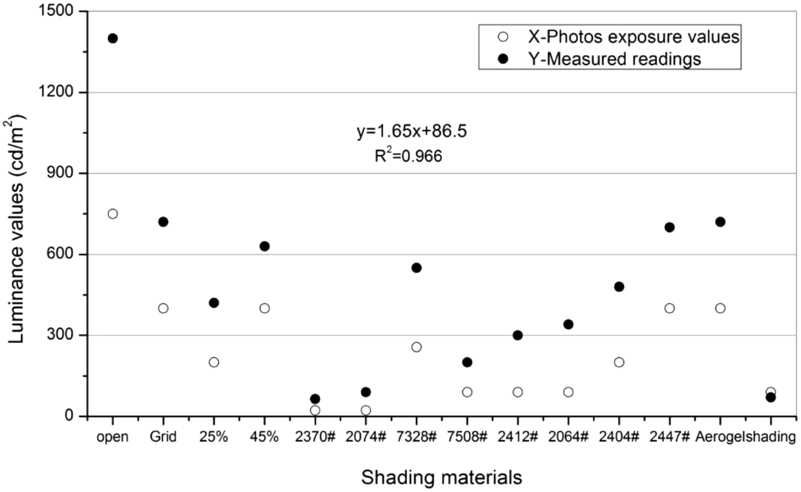

The parametric calibration model

The calibration models for luminance predicted by programs Flamingo rendering, DIVA and Lightscape were obtained by linear regression using the data from the box tests. The results are displayed in Figure 12 and represented by equations (1) to (3).

Figure 12.

Calibration model of different programs for box tests.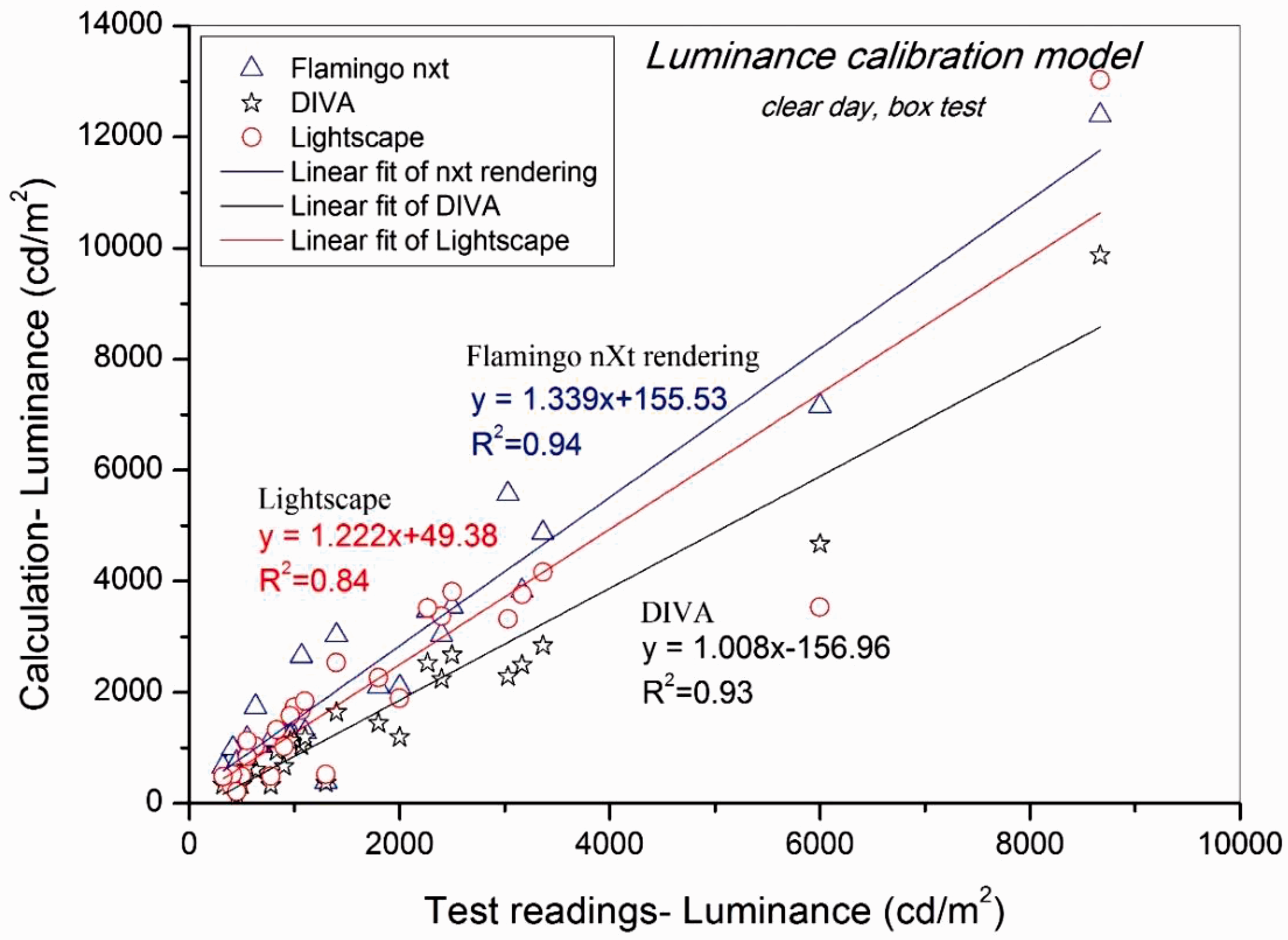

For Flamingo nXt rendering

y = 1.339 x + 155.53 R^{2} = 0.94

(1)

For Lightscape

y = 1.222 x + 49.38 R^{2} = 0.84

(2)

For DIVA

y = 1.008 x - 156.96 R^{2} = 0.93

(3)

where y is the corrected luminance in (cd/m²) and x is the calculated luminance from the software (cd/m²).

Figure 12 shows clearly that the results predicted by DIVA were the closest to the measured data with the slope of 1.008. The parametric models derived based on the box tests can be evaluated by the three programs.

The prediction error for each program

In order to provide a more holistic analysis of the differences between the simulation programs with the measurements, the mean and standard deviation of the calculation errors for each program were calculated. The measured luminance values were taken as the reference, as shown in Figure 13. For Flamingo nXt rendering, DIVA and Lightscape, mean±standard deviation were 763.0 ± 171.4, 143.4 ± 94.8 and 446.7 ± 206.7, respectively. In this paper, the luminance values for rendering pixels were shown to have the relatively higher error due to overestimation of the daylight penetrating through into the box. DIVA produced the lowest error (the error of luminance Δ_luminance = 143.4 cd/m²) for predicting the light distribution.

Figure 13.

Mean and standard deviation values of calculation error of different programs.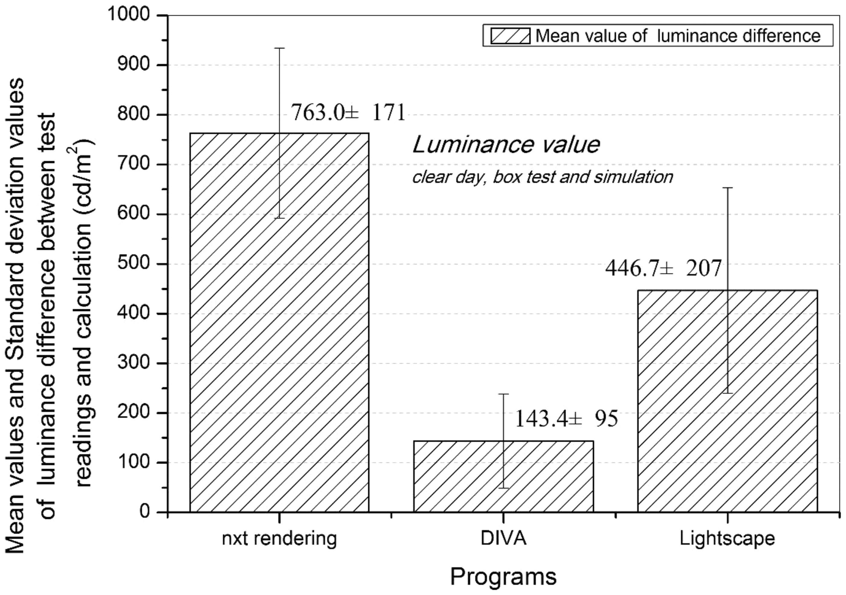

Discussion

There are numerous methods which could be used to define the sky conditions. Researchers have proposed many methods to predict sky luminance distribution. Due to the high costs of installation and maintenance, only a few ground stations have been set up worldwide to scan the sky and record the lighting distribution inside the surface and box.²⁵ During the field tests, the sky condition changes by hour and season. Although three sky conditions based on the CIE standard can be classified by the cloud index: n > 0.38, 0.13 ≤ n ≤ 0.38 and n < 0.13, respectively, corresponding to overcast, partly cloudy and clear sky condition, the sky condition during the tests could not be exactly represented in the simulation programs.

The field study under cloudy days was largely affected by the cloud index. If the indoor light environment is observed, the appropriate way is to consider the worst case where the overcast is selected as the ideal cloudy condition. However, this condition could not be designed and achieved during field measurements. The computer simulation method shows its particular advantage. Based on the previous research, this condition was utilized for lighting analysis.^5,23 This work using this method was to explore the accuracy of the programs and to obtain the appropriate parametric model to calibrate the results on the basis of validation process. This work was demonstrated by the previous research to be effective and necessary.²⁶ By analysing the algorithms used in the listed programs, the path tracing would provide more accurate results compared with others, because it includes the entire model (Global Illumination). However, the validation method used in this study may overestimate the illuminance. The best way to get the difference is to simulate a shadow cast on the surface being measured and compare the results with a physical model that also has a shadow on it. The shadow condition could be compared to the measured sky with clouds, and the relationship between illuminance values under cloud cover and then simulation values would be obtained. Based on this, in Flamingo the sky component (with no sun) is regulated infinitely from 0% to 100%, so it could be reduced to simulate more realistic conditions.

According to these experiments, the higher accuracy calibration models could be built up. Compared with the inconvenience and non-realistic tests in real buildings, these parametric models would provide an effective way to predict the lighting performance inside the buildings by using the simulation programs. On the one hand, this method could demonstrate the details of the useful lighting distribution for design; on the other hand, it would significantly reduce the test time and efficiently avoid the troubles caused by real time and real place measurement. However, there are still some limitations in this study. The field measurements, which simulated the situation on several angles in a whole year by rotating the model in the real test day, could just only provide the physical simulation results. The conclusion has been stated that there are many large differences between the real sky conditions for scale model measurements and the CIE sky conditions for computer simulations.²⁷ As a bridge, the correct factor between actual measurement and physical simulation is necessary to be investigated. The values obtained by regression were taken as the adjustment factor in the test condition. The actual tests are necessary to correct this factor for different sky component and actual ground reflection. Furthermore based on the computer technologies, the correct factors could be obtained for design purpose.

There are also other issues that need further investigation to improve the accuracy of the models. Seen from the calibration models obtained from surface test and box test, the significant parametric difference can be found from the formulas. Theoretically, there should be no difference between these two models, because for the test conditions, the methodology and simulated conditions in the selected programs were maintained identically. The best way to explain this huge difference should be by physical models. The light properties, such as reflection and refraction, could vary depending on the surface or the surrounding and even the configurations. Any variation in these elements would accompany by a change in the light transmission. The particular building configurations could affect the regression of parametric model for simulation programs calibration, as well as the adjustment factors for actual physical tests. This experience has provided the firm evidence to build the scaled physical model which is necessary to provide guidance for the designers and engineers to accurately understand the lighting behaviour for model simulations.⁵

Conclusion

Based on the field measurements and simulation performed within different lighting analysis programs, following conclusions can be drawn.

The difference on parametric model between plate test and box test suggested that the scaled physical model was necessary for exploring the actual lighting performance of window configuration.

For clear sky condition, the parametric model could be deduced with high accuracy which supports the daylight design decision for building forms of various complexity by simulation.

Due to the cloud ratio of the overcast, the mathematic model should be adjusted to reach the high consistency between field tests and computer simulations.

Lighting simulation programs, such as Lightscape and climate-based DIVA, as well as rendering software Flamingo nXt could be suitable for lighting prediction. Among these programs, the DIVA program provides the lowest errors compared with the measured data for the physical model. The Flamingo nXt would give higher accuracy prediction for the plate tests.

Footnotes

Authors' contribution

All authors contributed equally in the preparation of this manuscript.

Acknowledgement

Also authors would like to thank Assoc. Prof. Mojtaba Navvab (The University of Michigan) and Kun Lai (Shanghai Jiao Tong University) for their support by providing the facilities for measurements and suggestions on the manuscript.

Declaration of conflicting interests

The authors declared no potential conflicts of interest with respect to the research, authorship, and/or publication of this article.

Funding

This work was financially supported by the (Key project of National Natural Science Foundation of China) under Grant (Number 51238005); and (the University of Michigan – Shanghai Jiao Tong University collaboration research fund) under Grant (Number U029504).

References

Mantzouratos

Gardiklis

Dedoussis

Kerhoulas

. Concise exterior lighting simulation methodology. Build Res Inform 2004; 32: 42–47.

Reinhart

Fitz

. Findings from a survey on the current use of daylight simulations in building design. Energy Build 2006; 38: 824–835.

DHW

Tsang

EKW

. An analysis of measured and simulated daylight illuminance and lighting savings in a daylit corridor. Build Environ 2005; 40: 973–982.

Bellia

Cesarano

Minichiello

Sibilio

. De-Light: A software tool for the evaluation of direct daylighting illuminances both indoors and outdoors – comparison with Superlite 2.0 and Lumen Micro 7.1. Build Environ 2000; 35: 281–295.

Galasiu

Atif

. Applicability of daylighting computer modeling in real case studies: Comparison between measured and simulated daylight availability and lighting consumption. Build Environ 2002; 37: 363–377.

Wong

Istiadji

. Effect of external shading devices on daylighting penetration in residential buildings. Light Res Technol 2004; 36: 317–333.

Linhart

Wittkopf

Scartezzini

J-L

. Performance of anidolic daylighting systems in tropical climates – parametric studies for identification of main influencing factors. Solar Energy 2010; 84: 1085–1094.

Wittkopf

Soon

EYY

. Analysing sky luminance scans and predicting frequent sky patterns in Singapore. Light Res Technol 2007; 39: 31–51.

Kleindienst

Andersen

. Comprehensive annual daylight design through a goal-based approach. Build Res Inform 2012; 40: 154–173.

10.

Darula

Kittler

Wittkopf

. Outdoor illuminance levels in the tropics and their representation in virtual sky domes. Arch Sci Rev 2006; 49: 301–313.

11.

Wittkopf

Yuniarti

Soon

. Prediction of energy savings with anidolic integrated ceiling across different daylight climates. Energy Build 2006; 38: 1120–1129.

12.

Rhinoceros Version 4.0, Service Release 8. 2010. Robert McNeel & Associates, New York, USA.

13.

Hinkel

. DIVA: an iterative method for building modular integrated models. Adv Geosci 2005; 4: 45–50.

14.

DIVA for Rhino Version 2.0. http://www.diva-for-rhino.com/, 2012–2015 Solemma, LLC.

15.

Purcell

Buck

Mark

Hanrahan

. Ray tracing on programmable graphics hardware. ACM Trans Graph 2002; 21: 703–712.

16.

Darula S and Kittler R. CIE general sky standard defining luminance distributions. In: Proc eSim. Montreal, Canada, 11–13 September 2002, pp.1–8.

17.

Neumann

. Radiosity and hybrid methods. ACM Trans Graph 1995; 14: 233–265.

18.

Christakou DE and Amorim CND. Daylighting simulation: Comparison of softwares for architect's utilization. In: Ninth international IBPSA conference, Montréal, Canada, 15–18 August 2005, pp.183–190.

19.

Lafortune E. Mathematical models and Monte Carlo algorithms for physically based rendering. Citeseer; 1996.

20.

Robison A and Shirley P. Image space gathering. In: Proceedings of the conference on high performance graphics, 7–9 August 2009. New Orleans, LA: ACM, 2009, pp.91–98.

21.

Volevich

Myszkowski

Khodulev

Kopylov

. Using the visual differences predictor to improve performance of progressive global illumination computation. ACM Trans Graph 2000; 19: 122–161.

22.

Baldasano

. Preliminary analysis of air quality data from large cities. Air Pollut IX 2001; 47: 173–182.

23.

Acosta

Navarro

Sendra

. Towards an analysis of daylighting simulation software. Energies 2011; 4: 1010–1024.

24.

Wittkopf

. Evaluation of virtual sky domes for the prediction of daylight performance with radiosity-based light simulation software. Arch Sci Rev 2005; 48: 173–177.

25.

. Predicting sky types and zenith luminance from the cloud index derived from geostationary satellite data. Light Res Technol 2012; 44: 139–148.

26.

Andersen

Kleindienst

Lee

Bodart

Cutler

. An intuitive daylighting performance analysis and optimization approach. Build Res Inform 2008; 36: 593–607.

27.

Kim

C-S

Chung

S-J

. Daylighting simulation as an architectural design process in museums installed with toplights. Build Environ 2011; 46: 210–222.