
Abstract
This study has two aims to investigate the energy demand response (DR) actions on thermal comfort and energy cost in detached residential houses (1960, 2010 and passive) in a cold climate. The first one is to find out the acceptable range of indoor air and operative temperatures complying with the recommended thermal comfort categories in accordance with the EN 15251 standard. The second one is to minimize the energy cost of electric heating system by means of the DR control strategy, without sacrificing thermal comfort of the occupants. This research was carried out with the validated dynamic building simulation tool IDA Indoor Climate and Energy. Three different control strategies were studied: A) a strategy based on real-time hourly electricity price, B) new DR control strategy based on previous hourly electricity prices and C) new predictive DR control strategy based on future hourly electricity prices. The results show that the lowest acceptable indoor air and operative temperatures can be reduced to 19.4℃ and 19.6℃, respectively. The maximum annual saving in total energy cost is about 10% by using the control algorithm C.
Keywords
Introduction
The building sector contributes up to 30% of global annual greenhouse gas emissions, primarily through the use of fossil fuels during their operational phase, and consumes up to 40% of all energy used. 1 The level of greenhouse gas emissions from buildings is correlated with the level of demand, supply and source of energy. Hence, due to scarcity of natural resources and continuous increment in the electricity consumption worldwide, it is very important as well as demanding to develop energy-saving strategies. The buildings in the European Union (EU) account for 40% of the total energy consumption, mainly in space heating and hot water. 2 Overall, residential and tertiary sectors in the EU account for 50% of the electricity consumption 2 : 22% of that consumption is for electric heating, 9% for hot water heating and 1% for air conditioning. 3 In Finland, due to its cold climate, the heating in residential buildings accounts for 22% of the total primary energy consumption. 4 In 2012, detached houses comprised 89% of the Finnish residential buildings 5 and 31% of their heating energy is obtained from electricity. 4
Better demand side management (DSM) and optimal control of heating, ventilation and air conditioning (HVAC) systems can reduce electricity demand and shift peak loads during shortage times. International Energy Agency (IEA) 6 states that control strategies such as pricing regulation, technical standards of demand response (DR) and environmental impacts by retailers or consumers form the main approach to relieve the global energy crisis. Callaway and Hiskens 7 showed that smart grid investments can demonstrate the potential for buildings to become grid-interactive resources while being just as controllable as or even more controllable than electricity generators. The smart grid concept proposes an electricity network that integrates generation and consumption with real-time two-way communications. 8 The US Federal Energy Regulation Communication (FERC) formulated the basic definition of DR. DR changes the electricity consumption patterns of end consumers to reduce instantaneous demand in times of high electricity prices. 9 DR relates to any programme which communicates with the end-customer about price changes in the market and their own energy use and encourages them to reduce or shift their energy consumption demand. DR actions also include load shifting and dynamic pricing control.10,11
Annala et al. 12 reviewed previous studies about acceptability of different kinds of DR for Finnish residential buildings and assessed the consumer’s awareness of the principle and benefits of DR programmes by two separate questionnaire studies. They suggested that price and security of supply are major motives to change consumption behaviour than environmental issues and that the savings expected to trigger any action may be relatively high. Surles and Henze 13 focused on utilizing a control analytic tool for evaluating the effectiveness of different DR actions to shift and reduce energy consumption during peak pricing periods and lower the total energy cost for residential homes and utilities. Residential DR is used and developed, in interesting ways, to improve systems' energy efficiency.14,15 Also, the same authors present a scheme for optimal performance of major household loads under smart grid context to get the benefits of the availability of variable tariffs and renewables. Ali et al. 16 optimized the DR control of partial storage electric space heating by using a linear programming approach to minimize the total energy cost of consumers. Thermal comfort was also taken into account by using assumed variation band of indoor temperature (±2.0℃). They concluded that combining the heat storage tank and thermal inertia of the house is able to offer much flexibility in DR control. Ali et al. 17 developed the research to find out the effect of storage tank’s degree on the flexibility of electric storage space heating load control and to analyze the impact of storage tank losses and demand uncertainty on the DR control optimality. In Álvarez-Bel and Escrivá-Escrivá, 18 there is a description of micro-grid management where the electricity supplied from the grid is integrated with the use of own renewable generation, more efficient resources, and demand resources connected to the micro-grid by means of an energy management and control system. Reductions of CO2 emission have been assessed for periods when renewable generation resources and demand management are cheaper than the electricity provided by the grid. Avci et al. 19 proposed a practical cost- and energy-efficient model for a predictive HVAC load control strategy for buildings with dynamic real-time electricity pricing. The temperature range of thermal comfort is determined by the user to keep the thermal comfort level at a reasonable range. They found significant reductions in total delivered energy and cost saving. Klein et al. 20 presented and implemented a multi-agent comfort and energy system to model alternative management for three different controller strategies and occupants. They model their case test by considering actual thermal zones, temperatures, occupant preferences and occupant schedules. They found differences between their model and the traditional predicted mean vote (PMV) thermal comfort evaluation for indoor comfort conditions and energy consumption which need more robust comfort standard. They finally achieved a 12% reduction in energy consumption and 5% improvement in occupant comfort in comparison with the baseline control strategy. Liu et al. 21 developed the multi-objective generic algorithm for model predictive control (MPC) to determine the optimal set point of heating and ventilation control system while improving indoor air quality. They found that the performance of the MPC controller with the optimized set points is able to reduce energy consumption by 5.2% in comparison to proportional-integral (PI) controller. Previous research has concentrated on residential DRs to address their actions in the residential sector while preserving indoor thermal comfort by means of temperature.22,23 Molderink et al. 23 presented a three-step control methodology on domestic energy streams by reshaping house energy profiles. They stated that objective like peak saving can be achieved without harming the comfort of residents since the indoor temperature deviation from indoor temperature set point is ±0.5℃.
Yoon et al. 24 proposed a controller strategy to save total delivered energy and cost while maintaining reasonable thermal comfort for two house models in Austin, TX, USA. The control strategy changes indoor temperature set point since the retail price is higher than the preset price of the customers; also, they used the range of indoor air temperature (22.0–25.0℃) for thermal comfort based on ASHRAE standard 55. 25 They stated that energy cost can be saved up to 10.8% by using this control strategy. Arteconi et al. 26 analyzed the influence of DSM control strategies on the performance of thermally activated building systems (TABS) for a commercial building. They analyzed three different DSM mechanisms to estimate its potential for load shifting requested by the electricity grid while maintaining thermal comfort by assuming specific indoor temperature range (19.0–26.0℃). They concluded high potential of TABS within the DSM framework.
According to the literature review, the indoor air temperature has been used until now as the main indicator for thermal comfort in DR studies. However, thermal comfort includes several other aspects like activity, clothing, humidity, air speed, surface temperatures and temperature drift. In this study, all these factors are accounted for, which is one of the novel features of this study. Further, two new control algorithms are used in the implementation of DR.
The lower and higher limits of PMV values are used to determine the acceptable minimum and maximum indoor air and operative temperatures. These temperatures are then determined, in accordance with the EN 15251 standard, 27 for the electric radiator heating system (ERHS) and electric floor heating system (EFHS) by on–off and P-controller types. Then, changing set point temperatures (air and operative temperatures) will be assessed by three different control strategies: A) a strategy based on real-time hourly electricity price (HEP), B) a strategy based on previous HEP and C) a strategy based on future HEP. The control strategies monitor and control space heating and reduce the peak load while maintaining thermal comfort of the occupants at acceptable levels.
Building description
The studied building type is a Finnish two-storey detached house (see Figure 1) simulated with three different levels of thermal insulation and thermal mass.
Two-storey building (180 m2) with area of each zone and window.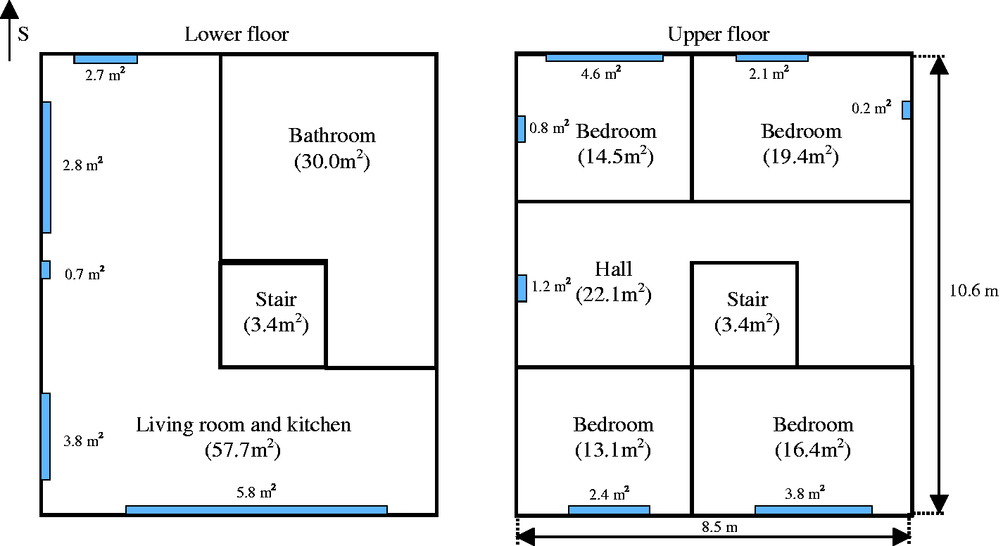
The floor area of the building is 180 m2, and it has six rooms and kitchen with the room height of 2.6 m. Nine different versions of the detached house were simulated, the versions being determined on the basis of differences in construction practice and building regulations during different decades.
Building types and properties
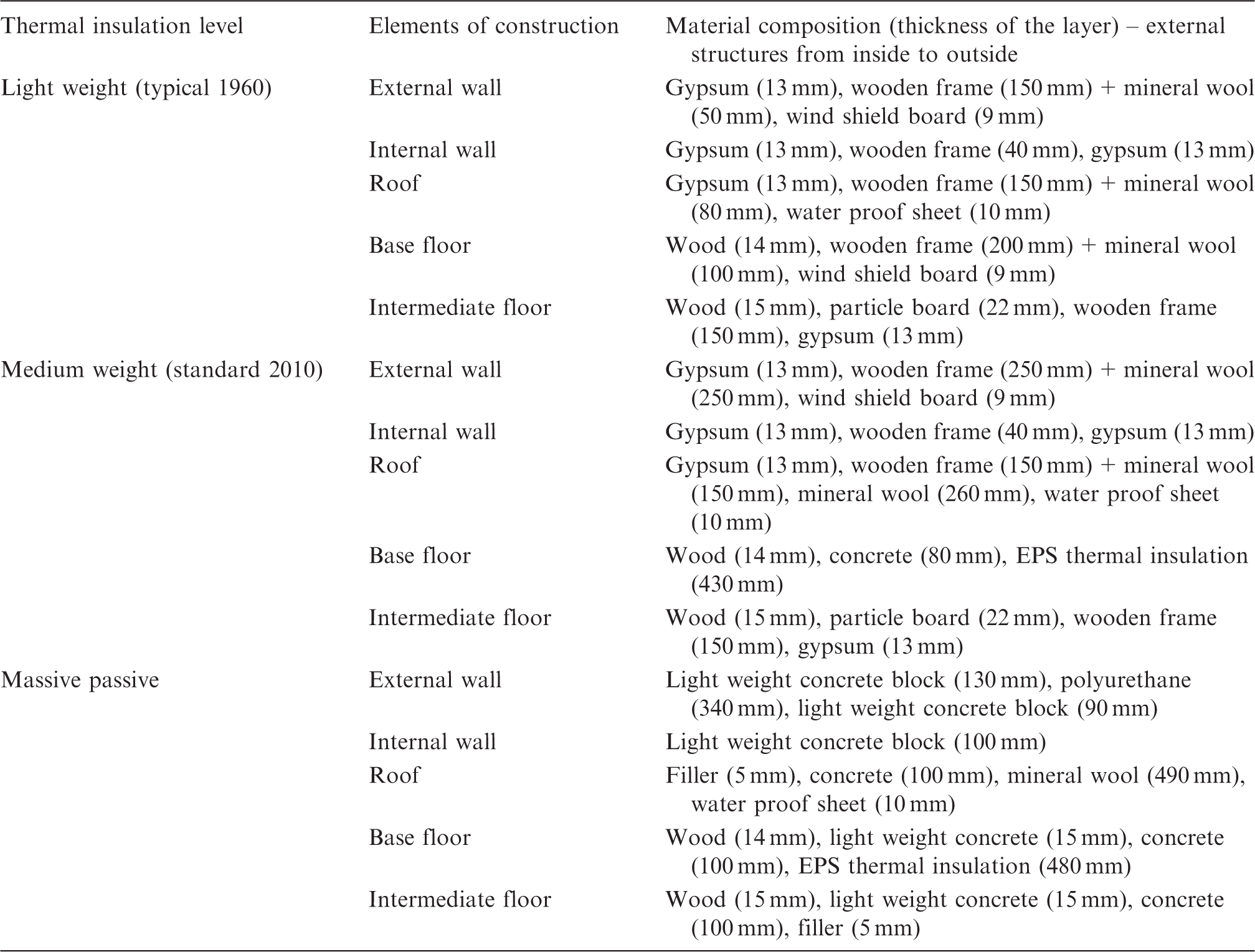
Building envelope specifications.
Properties of different structures: thermal insulation, U-values, window properties and air tightness.
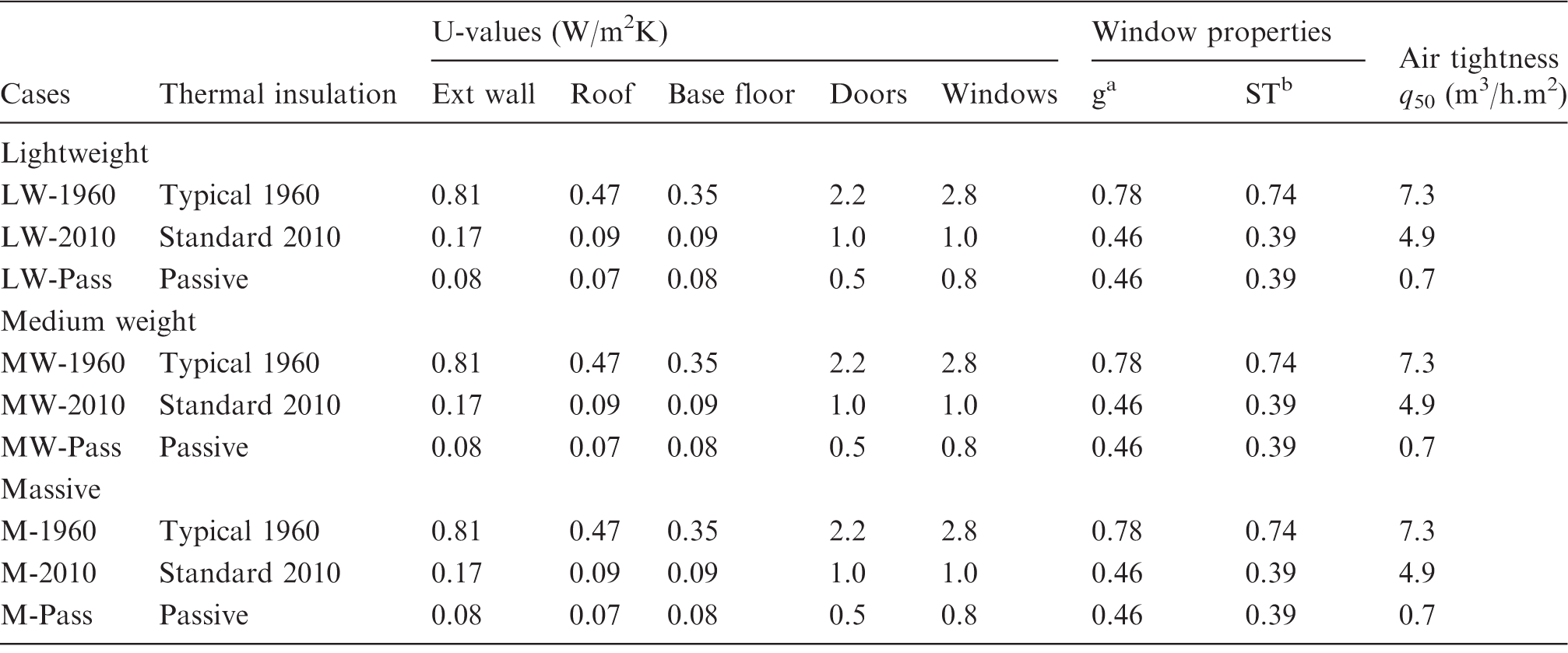
Total solar heat transmittance (g).
Direct solar transmittance (ST).
Heating and ventilation system
This research deals with the ERHS and EFHS, focusing on these two heat distribution systems and two typical controllers for electric heating systems (on–off controller 31 and P-controller 32 ) as the alternative systems and controller types for buildings. The value of the on–off controller type dead band is assumed to be 1.0℃ and the proportional band of the P-controller type is also assumed to be 1.0℃.
In addition, the ventilation system of different building types is studied. The 1960 building type has a mechanical exhaust ventilation system. The ventilation rate of this building type is based on the average ventilation rate of 55 Finnish houses with mechanical exhaust ventilation. 33 For the 1960s cases, the ventilation rate considered is 0.36 air change per hour (ACH). The 2010 and Passive building types have a mechanical supply and exhaust ventilation system with heat recovery. The system of mechanical supply and exhaust ventilation with heat recovery is the most common ventilation system in new Finnish detached houses. Heat recovery with the efficiency of 60% and 80% for 2010 and Passive cases, respectively, has been employed. In the 2010 and Passive building types, ACH is 0.5, in accordance with the guideline of the Finnish building code D2 (2012). 34
Behaviour of the occupants
Activities and clothing have an effect on thermal comfort.35,36 Thus, the activity levels of 1.0 met (seated and relaxed) and 1.2met (standing and relaxed) are used in the simulation and clothing insulation levels of 0.96 clo (trousers, long-sleeved shirts plus suit jackets) and 1.14 clo (trousers, long-sleeved shirts plus suit jackets plus vest and T-shirt) are studied. 37
Because the relative humidity of indoor air also affects thermal comfort,38,36 indoor air moisture is considered in the simulation. Thus, typical Finnish level of moisture production was used as initial data for the simulation. This study used the daily moisture production of 2.7 kg/24 h per occupant, in accordance with the study by Vinha et al. 39 ; therefore, the total moisture production from persons and equipment is 10.8 kg/24 h and 5.4148 kg/24 h (0.00006267 kg/s), respectively.
Internal heat gains are considered as an important component in heating load production in buildings. They consist of sensible and latent heat gains from occupants, sensible heat gains from lighting, and sensible and latent heat gains from equipment. The heat gains from occupants were considered when studying different activity levels, but the value of internal heat gains from lighting and equipment still needs further study. To implement these values, typical consumption profiles of appliances and lighting of Finnish detached houses are used in this study.
This study utilizes consumption profiles defined by means of the conditional demand analysis (CDA) technique
40
and applied to 1630 Finnish households. The analysis was carried out by using statistical information gathered through questionnaires and by examining one-year hourly measured electricity consumption of the households. The analysis resulted in different consumption profiles for weekdays and holidays of the four seasons of the year. The hourly consumption profiles for the equipment and lighting used in the simulation are presented in Figure 2 for winter weekdays.
Hourly electric power for lighting and equipment in a typical Finnish household during weekdays of the winter period.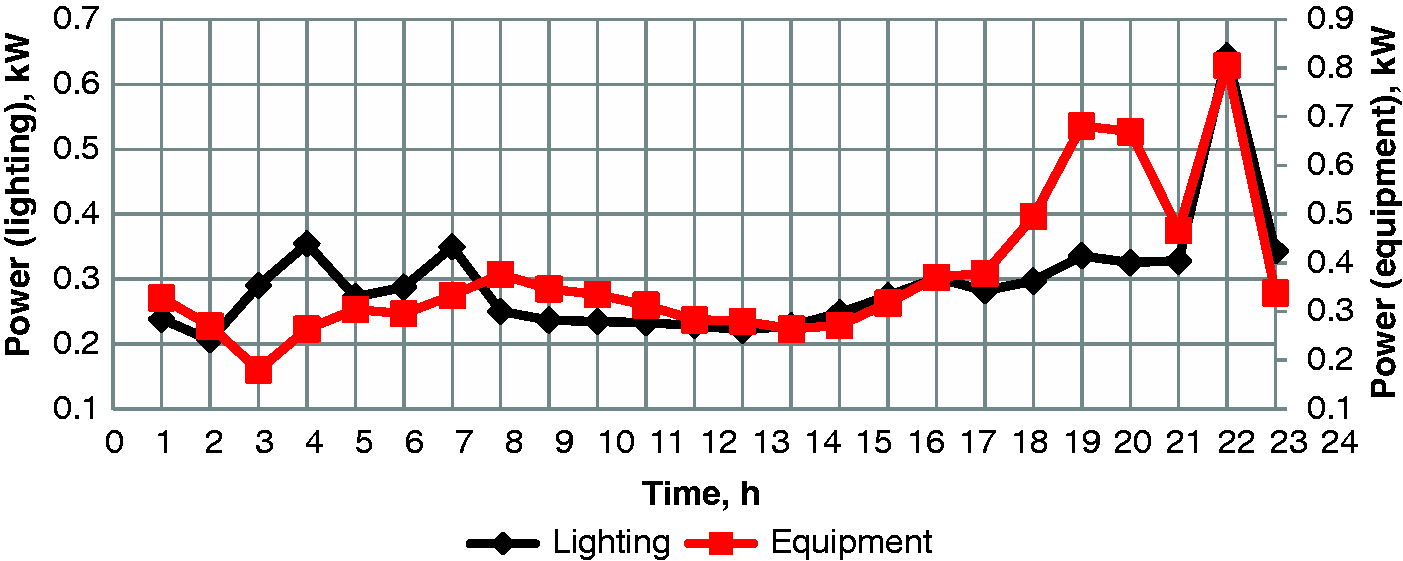
This research assumed that all the electric energy used for inside lighting and part of the electric energy used for equipment end up as an internal heat gain of the building.41,42 In accordance with a guideline of the Finnish building code, 43 a half of the electricity consumption of the equipment that heat water (e.g. dishwasher or washing machine) can be assumed to end up as internal heat gain of the building. Because of this, 86% of the total electricity consumption of the equipment was assumed to end up as an internal heat gain of the studied houses. According to hourly consumption profiles for lighting and equipment, these values for the studied buildings are 8.5 and 22.2 KWh/(m2.a.).
Methodology development
The study structure
Figure 3 shows the study structure consisting of two main parts, including control algorithm and the IDA ICE building simulation software (see “The IDA ICE simulation tool” section). The control algorithm part receives three different inputs from acceptable indoor temperature set points (see “Defining minimum and maximum of indoor temperature set points” section), weather file (see “Weather data” section) and HEP. The IDA ICE receives two different inputs from control algorithm and input data. Input data part comprises information about building geometry, envelope, glazing, HVAC systems, lighting, equipment, heating system, etc. Finally, the IDA ICE produces output data (e.g. total delivered energy and cost) by using control algorithm data and input data simultaneously.
The flow chart of the study.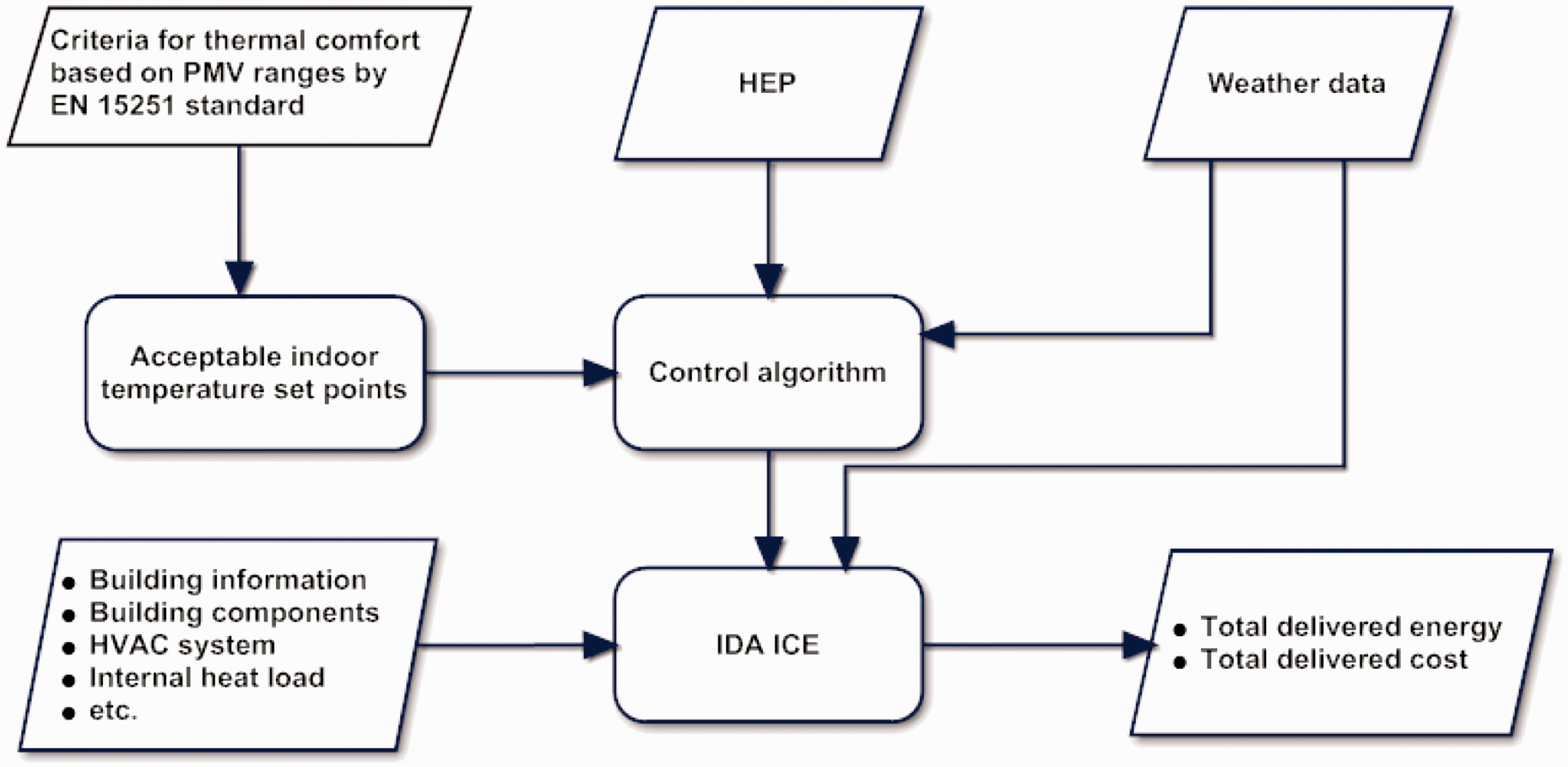
Indoor thermal comfort according to related standard
Thermal comfort describes a person’s psychological state of mind which expresses satisfaction with the thermal environment and is assessed by subjective evaluation. 44 Thermal comfort has great influence on the productivity and satisfaction of occupants in buildings. 45 This study uses the Fanger approach to predict the thermal comfort of occupants in buildings. 44
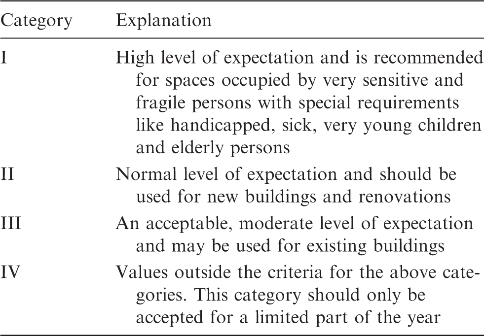
To conduct this research, two reference standards including the EN 15251 27 and ASHRAE standard 55 2 5 were considered. EN 15251, the European standard, specifies the indoor environmental parameters which have an impact on energy performance of the buildings. Through energy simulation, a study and analysis have been carried out to satisfy the thermal conditions for different categories defined in that standard. 27
Description of the applicability of thermal comfort categories of the EN 15251. 27
Thermal comfort categories for design of mechanically heated and cooled buildings. 27
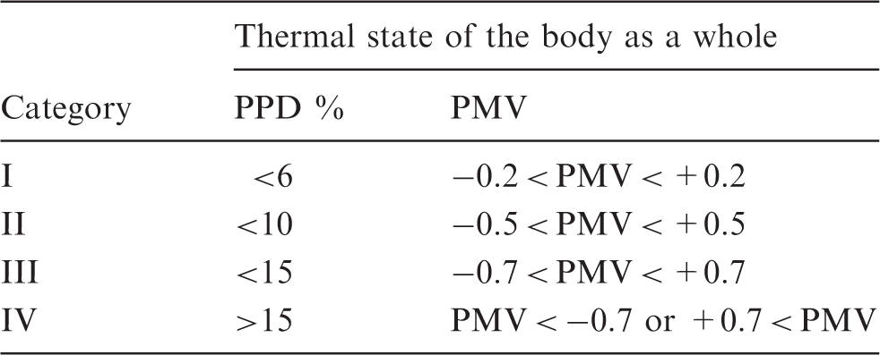
Moreover, the categories in Table 3 and Table 4 are defined by means of PPD and PMV values, and the lower limits of PMV values were used to determine the minimum acceptable indoor air and operative temperatures during the heating season. The maximum PMV values were used to define the maximum acceptable indoor air and operative temperature during the heating season, even though the maximum PMV values have originally been defined for the cooling season.
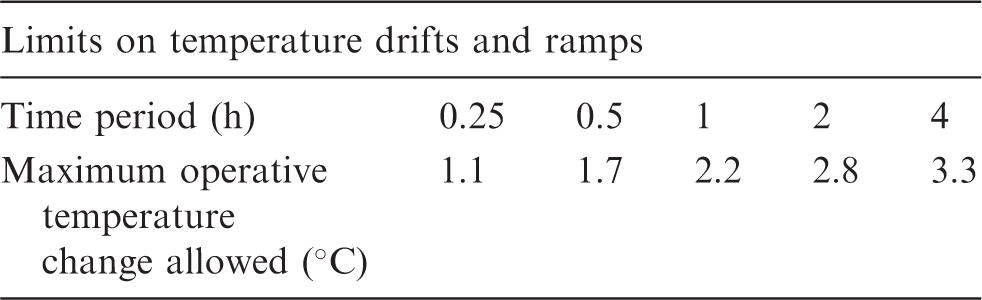
Maximum allowed variation in operative temperature. 25
Defining minimum and maximum of indoor temperature set points
In order to determine the acceptable range of indoor air and operative temperatures, the correlation between PMV values and indoor temperatures was studied. The coldest period (8 January–4 March) was simulated to determine the critical values of PMVs (minimum and maximum) and indoor temperatures. PMVs and indoor temperature obtained were drawn to find the linear trendline of PMV as a function of indoor temperature. The defined linear trendlines were used to determine the acceptable range of indoor temperatures by inserting the minimum and maximum PMV values of the thermal comfort categories into the equation of linear trendlines. This strategy was simulated to find out the acceptable range of indoor temperatures for different building types with different heat distribution systems and different activity levels, clothing levels and air velocities. Figure 4 shows an example of minimum and maximum lines of indoor air temperatures (Tair) for the LW-1960 building type with ERHS and P-controller type.
Defining minimum and maximum linear lines of indoor temperature set point in different categories.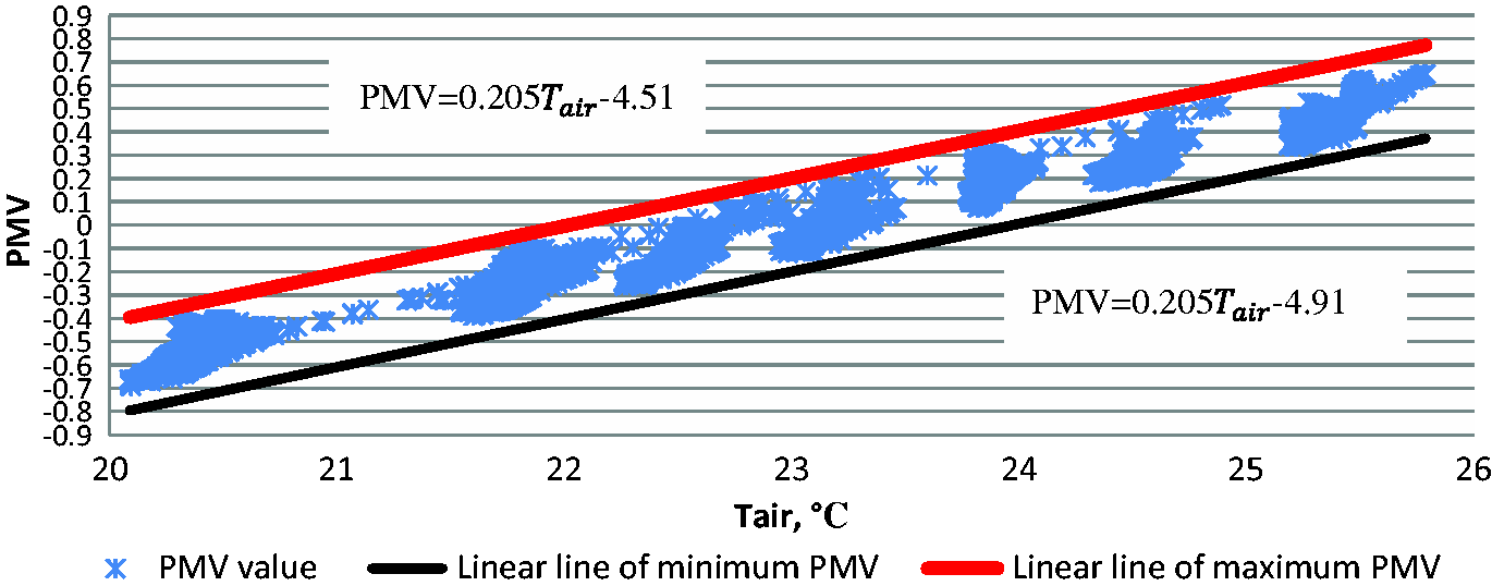
The IDA ICE simulation tool
The simulation part of this research was implemented by IDA Indoor Climate and Energy (IDA ICE). 46 The IDA ICE 4.5 building simulation software is a detailed and dynamic multi-zone simulation application with variable time step for the study of ICE. The IDA ICE was validated against the EN 15265-2007 standard 47 and the maximum inaccuracy levels for heating and cooling demand were 8% and 11%. The IDA ICE has been validated in several studies48–51 which show good justification to use the IDA ICE in this study. For example, Travesi et al. 52 conducted an empirical validation study of models of the IDA ICE relating to thermal behaviour of buildings and HVAC equipment. They found that agreement between simulated and measured data was good and disagreements were similar to the measurement uncertainty.
The IDA ICE is a befitting tool for simulation of energy consumption, indoor air quality and thermal comfort in buildings. It can be used for a variety of applications, such as integrated airflow network and thermal models, CO2 and moisture calculation and vertical temperature gradients.
Weather data
This research used the Finnish test reference year (TRY2012) as a weather data for dynamic simulations. The data consists of detailed hourly data of temperature, relative humidity, wind velocity, and solar direction and radiation describing the current climatic conditions of Southern Finland. The data on weather conditions were accumulated and computed by recording a 30-year period (1980–2009) in Helsinki region. 53 Finnish climate is highly influenced by the country's geographical position between the 60th and 70th northern parallels in the Eurasian continent's coastal zone, which shows characteristics of both a maritime and a continental climate, depending on the direction of weather front. The annual average temperature for Helsinki-Vantaa region is +5.4℃, bringing the region under climatic zone 1. 54 The average number of degree days at indoor temperature of 17.0℃ is 3952 Kd.
Simulated DR control strategies
In the DR mechanism studied, the customers are motivated to respond to the HEP 55 by changing the indoor temperature set point of space heating to decrease the total energy cost while maintaining the thermal comfort of occupants at the acceptable level. The DR control algorithm for controlling the electric space heating has different levels of complexity and requisites. Using electricity price as an incentive, the three proposed control algorithms unleash the flexibility of DR. These control algorithms are the extension of the conventional on–off control which use the real time HEP, the previous HEPs or the future HEPs. To investigate the effect of each control algorithm on total delivered energy and energy cost of studied detached houses, these control algorithms are applied with IDA ICE 4.5.
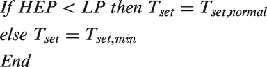
Control algorithm A
This is the simplest algorithm which controls indoor temperature set point (Tset) according to HEP. To change the set point, if the HEP is less than limiting price (LP), the normal indoor temperature set point is used; otherwise, it will be the minimum set point in the acceptable temperature range. The pseudo code (1) for the control mechanism is as given in equation (1):
Control algorithm B
The main idea of this new control algorithm is to manage the indoor temperature set point according to previous HEPs. This is done by comparing the median of previous hourly electricity prices (MHEP) and current HEP. The number of previous hours can be selected, and the optimal number of previous hours is analyzed in this study. At every hour when the new price of the Nord Pool
56
trading system is announced, the DR control modifies the indoor temperature set point according to HEP, which can be either increased, kept constant or decreased. The control algorithm has two parts: the first part compares MHEP and HEP, and the second part concentrates on the indoor temperature and outdoor temperature trend. The pseudo code (2) for the control mechanism is as given in equation (2):
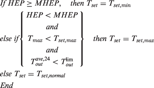
In this control algorithm, if HEP is higher than or equal to MHEP, the indoor temperature set point is decreased, otherwise the indoor temperature set point is either increased or the normal one is used, depending on the indoor temperature and outdoor temperature trend. The indoor temperature is compared with constant parameter Tset,max to avoid overheating. Then, to find out whether the outdoor temperature is getting colder or warmer, the average outdoor temperature of the previous 24 h is compared by the limiting outdoor temperature. If the maximum indoor temperature of the building is less than the maximum indoor temperature set points, acceptable or lower one (see “Acceptable indoor temperature set points” section), and the outdoor temperature is lower than the limiting outdoor temperature, the indoor temperature can be increased. Otherwise, the normal indoor temperature set point is used.
In order to improve the performance of the algorithm, the optimal number of previous hours was examined. These numbers of previous hours, ranging from 2 to 24 h, were then used by the algorithm to simulate the annual energy cost of space heating (ECSH) of the building. Figure 5 shows the effect of previous hours on the ECSH for massive passive (M-Pass) building type simulated with HEP of three years (2010–2013). Because the HEP of 2011 is quite similar to the HEP of 2012, it was not studied; and the HEP of 2010 and 2012 or 2013 are quite different. Figure 5 shows results in two price scales. For minimizing the ECSH for the studied building types, the optimum number of previous hours among the studied time periods is 14. Moreover, it was found that the level of thermal insulation and thermal mass of the building does not affect the resultant optimum number of hours. Also, the optimum number of previous hours is independent of the studied time period and building types. Furthermore, the optimal number of previous hours does not depend on the heat distribution systems and temperature controller types studied.
Total energy cost of space heating in M-Pass building (see Table 2) with different number of previous hours, which have been used in the algorithm B.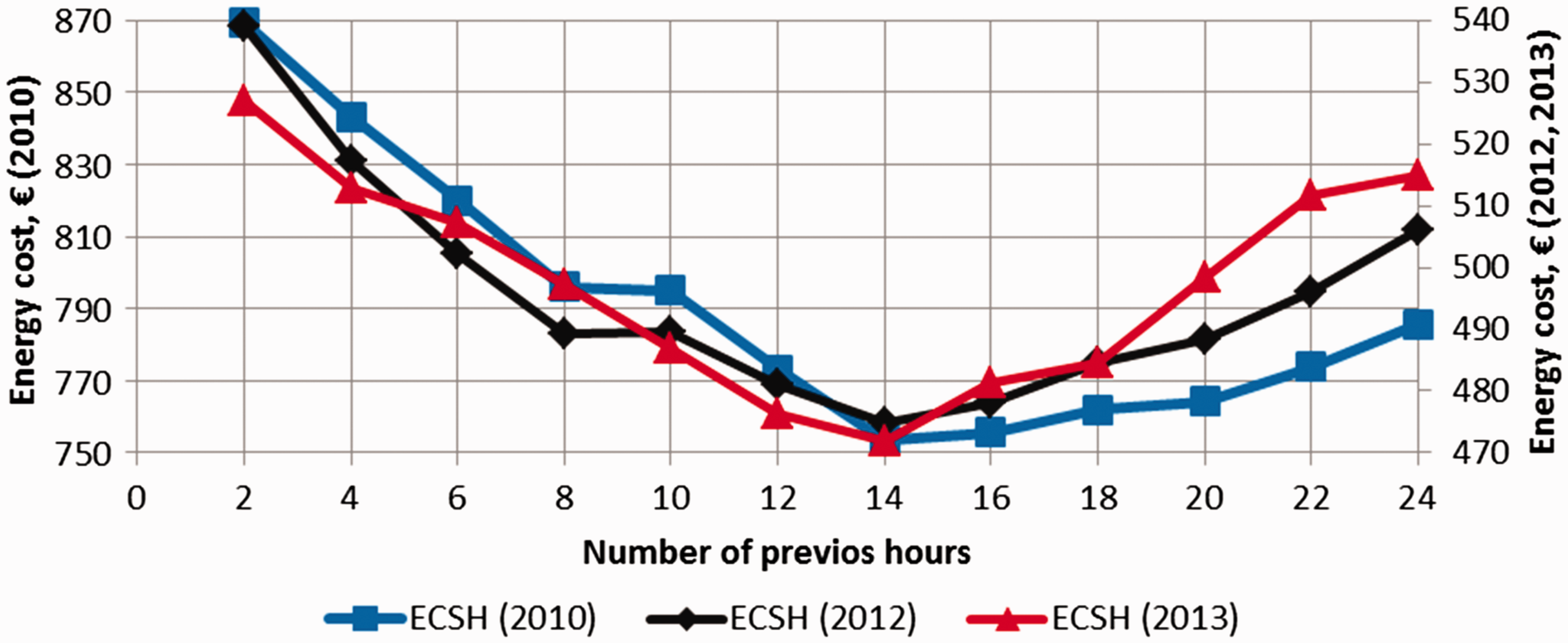
These results were simulated for LW-1960 and M-Pass building types with ERHS and P-controller type. The normal indoor temperature set point was 21.0℃,49,52 the limiting outdoor temperature (
Control algorithm C
The principle of this new predictive control algorithm is to control the indoor temperature set point by adjusting it in accordance with future hourly prices. This algorithm generates a control signal (CS) by utilizing maximum subarray problem. The maximum subarray problem calculates a contiguous subarray which has the largest sum within a one-dimensional array of numbers, containing at least one positive number. 57 By means of this concept, the HEPs can be accordingly sorted to realize their rising or falling trend; hence, corresponding CSs can be assigned to the limited future prices.
This control algorithm has two parts: first, the control algorithm calculates the CS; second, the indoor temperature set point of building is controlled according to the CS, the indoor temperature and outdoor temperature trend (the indoor temperature and outdoor temperature trend rules are similar to the rules used with control algorithm B).
The principle of such control algorithm is: the algorithm generates CS = +1 to increase the indoor air temperature set point to the maximum one before the HEP increases. As soon as the HEP starts to increase, the algorithm generates CS = −1 to decrease the indoor air temperature set point to the minimum one. In other conditions, the algorithm generates CS = 0 and the indoor air temperature set point is the normal set point temperature. The pseudo code (3) of the control mechanism is as given in equation (3):
Total energy cost of space heating in M-Pass building (see Table 2) with different number of future hours which have been used in the algorithm C.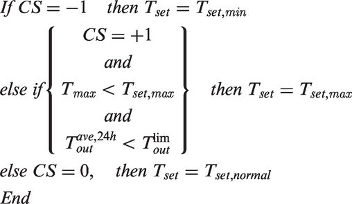

Results and discussion
The results present an assessment of the indoor operative temperature changes to find out the level of fulfilment of the ASHRAE standard 55. 25 Then, the acceptable indoor air and operative temperatures are presented in accordance with the EN 15251 standard 27 for the LW-1960 and M-Pass building types as the extreme ones. Finally, the control algorithms are applied in the on–off and P-controller types for ERHS and EFHS.
Fulfilment of the ASHRAE standard 55
To assess the speed of the indoor operative temperature drift in the nine studied buildings, Figure 7 shows the indoor operative temperature during 4 h of January (as typical winter temperatures in Finland) since the heating system is switched off. It shows that LW-1960 and MW-1960 buildings do not fulfil the ASHRAE standard 55,
25
the variation of the indoor operative temperature exceeding the allowed variation. The ASHRAE standard 55
2
5
states that higher variations may be acceptable because the studied temperature variations are created by the control system. The LW-1960 building was selected for the energy and cost simulations because it represents the extreme building type due to the very low thermal mass and poor level of thermal insulation.
Fulfilment of ASHRAE standard 55 rule for operative temperature change for the nine studied buildings.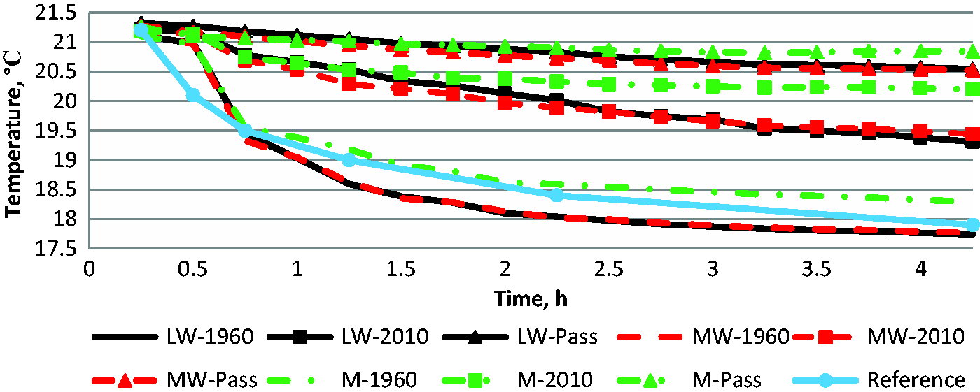
Acceptable indoor temperature set points
The acceptable indoor temperature set point depends on various conditions such as different occupants’ behaviour (e.g. different met levels and different clothing levels), heat distribution systems and the controller types installed in different buildings. To find out the influence of these conditions on acceptable indoor temperatures, this research studied different activity levels, clothing levels and air velocities.
Minimum and maximum of air and operative temperatures in ERHS and EFHS with on–off controller and P-controller types for LW-1960 and M-Pass building types (the activity and clothing levels are 1.2 met and 0.96 clo, and air velocity is 0.1 m/s).
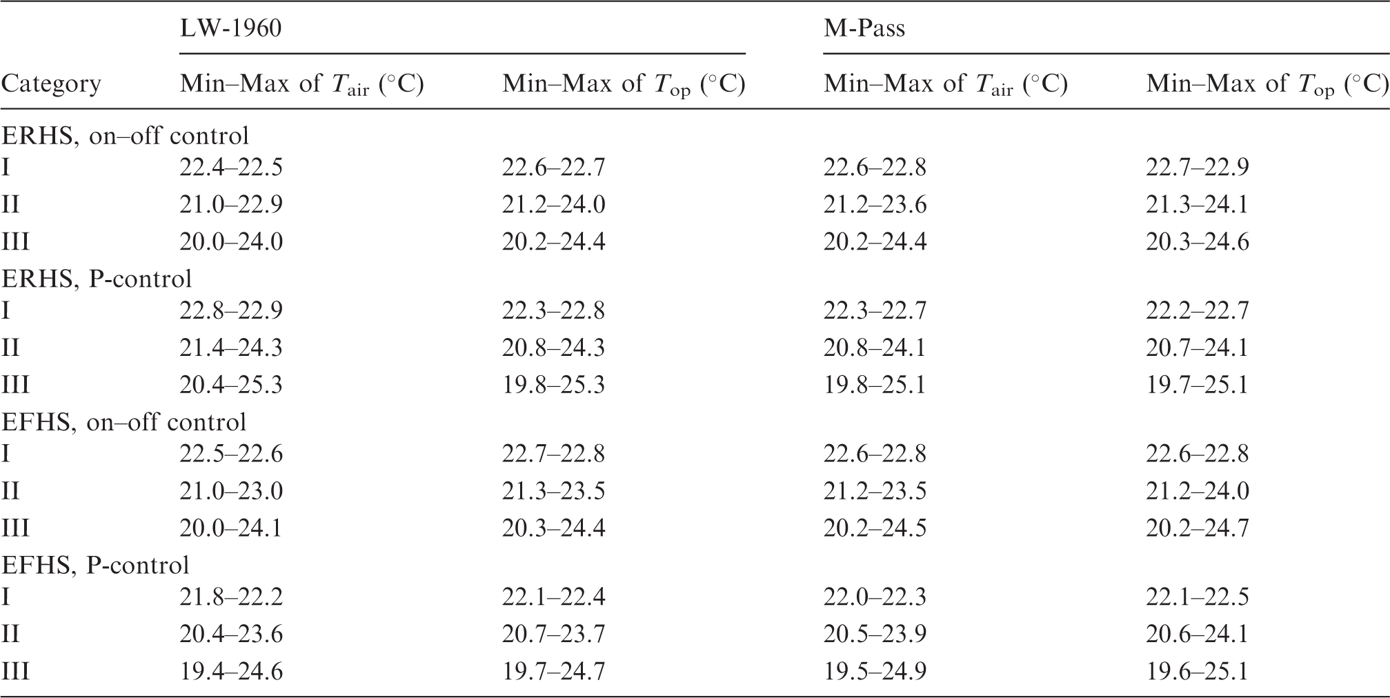
The lowest minimum indoor air temperature set points for category I, II and III are 21.8℃, 20.4℃ and 19.4℃, respectively, and the minimums of indoor operative temperature set points for categories I, II and III are 22.1℃, 20.6℃ and 19.6℃, respectively. In all the studied cases in category III, the minimum indoor air and operative temperature set points are lower than the normal set point temperature used in detached houses in accordance with the Finnish building code (21.0℃), but in some of the studied cases from category II are lower than the normal set point temperature. Thus, the results indicate that the thermal comfort category III of the EN 15251 standard 27 can be used for control algorithms. The decrease in the range of indoor temperature set points of thermal comfort from category III to category I indicates smaller fluctuation from indoor temperature set points. The decreasing fluctuation of indoor temperature set point verifies the increasing expectation levels of occupants.
The calculated minimum operative temperature set points imply that these values are higher than the recommended one by the EN 15251 standard 27 (18.0℃) for living spaces of residential buildings in category III. Also, the maximum operative temperatures are either lower or higher than the recommended maximum indoor temperature set point defined by the EN 15251 standard 27 (25.0℃). Therefore, the recommended minimum operative temperature set point of the EN 15251 standard cannot be used for such acceptable minimum temperature set points in the studied cases.
The maximum and minimum temperature decreases from the normal set point are 1.6℃ and 0.6℃ calculated for the LW-1960 building type by using EFHS and ERHS with the P-controller type. Such decreases prove the potential of changing indoor temperature set point to achieve lower total delivered energy and energy cost in comparison with using a normal set point temperature for the whole year. Also, the highest temperature increase, 4.3℃, from the normal set point occurred in the LW-1960 building type using ERHS with the P-controller type; however, the lowest one is 3.0℃ and calculated in LW-1960 where both ERHS and EFHS with the on–off controller type were used. The difference of the minimum indoor air temperatures between LW-1960 and M-Pass building types is insignificant. But, in most of the studied cases, the maximum indoor air temperature for M-Pass building is a bit (0.1–0.7℃) higher than the LW-1960 building types. Thus, the range of acceptable indoor air temperatures for the M-Pass is wider than LW-1960 building type, which means thermal mass and insulation are slightly effective on this range. The results of most of the studied cases show that increasing thermal insulation slightly increases the acceptable indoor temperature ranges. Also, in the same controller system, the different heat distributions are insignificant in the acceptable indoor temperature ranges; however, the range of acceptable indoor temperature set points of the P-controller type is wider than that of the on–off controller type.
In the on–off controller type cases, the differences between indoor air and operative temperatures are insignificant. But, smaller fluctuation of the indoor temperature in P-controller type cases causes more differences between indoor air and operative temperatures.
The results show that the minimum indoor temperature set points in ERHS with the P-controller type are higher than with the on–off controller type, which can be the reason for the fluctuations in the indoor temperature with the on–off controller type. But, the minimum indoor temperature set point in EFHS with the P-controller type is lower than with the on–off controller type.
This research assessed influence of acceptable indoor temperature on different activity levels, clothing levels and air velocities, including the velocities of 0.1 m/s and 0.2 m/s, because they are typical air velocities in detached houses.58,59 The effect of air velocity depends on the thermal comfort category; it means that by changing the air velocity from 0.1 m/s to 0.2 m/s, the minimum indoor air and operative temperature set point for categories I, II and III, shown in Table 6, increase from 0.6℃ to 1.0℃ depending on cases. The effect of activity level also depends on the thermal comfort category: the minimum indoor temperature set point can be increased up to 2.0℃ for categories I and up to 2.5℃ for category II or III by changing the activity level from 1.2 to 1. Moreover, the effect of a change in clothing level from 1.14 clo (shown in Table 6) to 0.96 clo is to increase the minimum indoor air and operative temperatures between 0.9℃ and 1.3℃.
Performance of control algorithms
The control algorithms were implemented in the IDA ICE. The pseudo code for each control algorithm was defined by the logic applications of IDA ICE, then the weather data and HEPs are called as the input values. In order to examine different control algorithms to find out total delivered energy and cost, the performance of each control algorithm is analysed. Figure 8 shows the operation of control algorithm A during the weekdays of the first week of February 2012 (see “Weather data” section). It shows the adjustment of Tset according to HEP; if the HEP is less than 50€/MWh, the normal indoor temperature set point is used; otherwise, the minimum indoor temperature set point will be used.
Operation’s results of control algorithm A for M-Pass building type.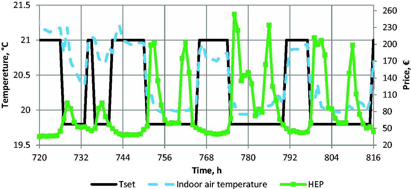
Figure 9(a) shows the operation of control algorithm B. It displays the adjustment of Tset according to other parameters. It displays the dynamic behaviour of changing indoor air temperature according to Tset (acceptable indoor temperature set points are presented in “Defining minimum and maximum of indoor temperature set points” section). Figure 9(b) illustrates that the comparison of indoor air temperatures for LW-1960 and M-Pass building types with indoor air temperature set point. It shows the dynamic behaviour of the LW-1960 building derived by changing indoor air temperature is faster than that of the M-Pass building. Because of the higher thermal mass and insulation, the changing indoor air temperature of M-Pass building type is so restricted.
Operation’s results of control algorithm B in different variables for M-Pass building type (a) and comparing indoor air temperatures for different building types with indoor air temperature set point (b).
Figure 10(a) shows the output signal of control algorithm C in accordance with the HEP. The control algorithm controls the set point of space heating by responding to the volatility of future prices. The prices are updated after certain hours. The operation of control algorithm C is shown in Figure 10(b). Also, the comparison between Figure 10(b) and Figure 9(a) shows that Tset (acceptable indoor temperature set points) is controlled quite differently and increased much less by control algorithm C. These results were simulated for an EFHS with P-controller type and the thermal comfort category III.
Output signal of control algorithm C with the HEP (a), and operation’s results of control algorithm C in different variables for M-Pass building type (b).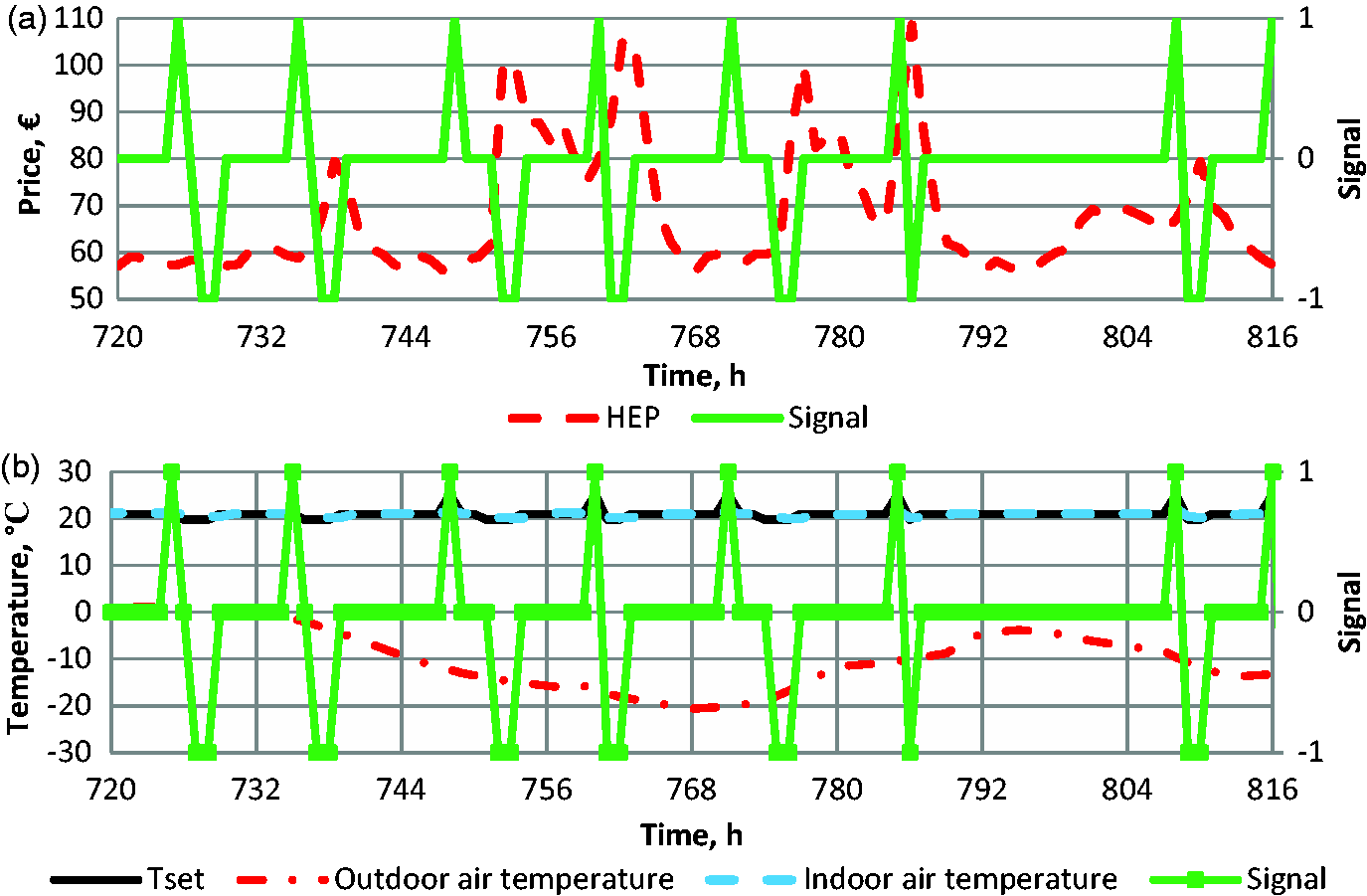
Breakdown of delivered energy consumption
Breakdown of delivered energy consumption of the LW-1960 and M-Pass building types.
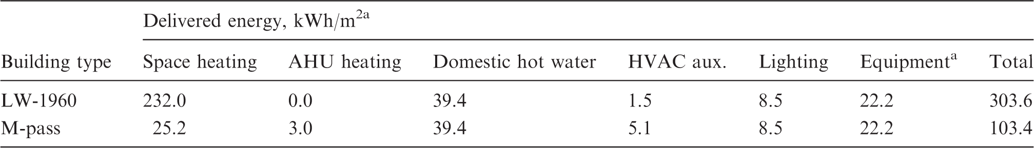
It is assumed 86% of the electricity consumption of equipment ends up as internal heat gain. 43
Total delivered energy and cost
Description of the simulation study
Results for the total delivered energies and energy costs of different set points and control algorithms for ERHS and EFHS with P-controller (P-C) and on–off controller (O-C) types with normal indoor temperature set point (21.0℃).

Reference cases with the normal indoor temperature set point
The results of the reference cases shown in Table 8 (without using the control algorithms) show that the total delivered energy and the energy cost of the LW-1960 building type are 3.0 and 3.3 times more than those of the M-Pass building types, respectively. Also, the results illustrate that the total delivered energy of the LW-1960 building type in EFHS is up to 7.4% higher than that of ERHS for both the on–off and P-controller types; the total energy cost of EFHS being 7.2% and 6.5% higher for the on–off and P-controller types, respectively. Also, the comparison results for the M-Pass building type reveal that the difference of the total delivered energy between ERHS and EFHS is small for on–off and P-controller types; but, the total energy cost of EFHS is 4.5% and 1.3% higher than ERHS for the on–off and P-controller types, respectively. In most of the studied cases, the total energy cost in M-Pass building type with the on–off controller type and in LW-1960 building type with the P-controller type are lower.
The minimum indoor temperature set point
In most of the studied cases, the total delivered energy and cost with minimum indoor temperature set point are the lowest ones without the use of control algorithms, but, in few cases (the M-Pass building type with EFHS used the control algorithm B and C in options of
The variable indoor temperature set point controlled by the algorithms
In most of the studied cases, the total delivered energy and cost are decreased for control algorithm B and C by two alternatives; the first one is to change the maximum indoor air temperature set point to a lower one (22.0℃) and the second one is to decrease the limiting outdoor temperature to the lowest one (−21.0℃). In most of the studied cases, the control algorithm B is more effective with different heat distribution systems, controller types and options of Tset,min and
The control algorithm B and C are able to save the total delivered energy and cost in most of the studied cases. But, depending on the values of the parameters and the controller type used with the control algorithms, the control algorithm B increases total delivered energy and cost by 5.4% and 26.1%, respectively; and the control algorithm C increases them by 3.6% and 20.7%, respectively in M-Pass building type with EFHS. This indicates that a performance of the control algorithms B and C is sensitive to the values of the parameters and the controller types.
When compared with the reference case, the maximum energy and cost saved by the use of control algorithm A are 0.8% and 2.1%, respectively. The control algorithm B can save total delivered energy and cost up to 3.1% and 7.7%, respectively. The maximum total delivered energy and cost saved by the use of control algorithms C are 1.3% and 9.6%, respectively.
Conclusions
This study investigated the acceptable range of indoor air and operative temperatures, complying with the thermal comfort categories recommended by the EN 15251 standard, for a detached house. Nine different houses, including three different insulation levels and three different thermal mass levels were simulated in the cold climate of Finland. The goal was to minimize the total delivered energy and cost of electrically heated detached houses by means of three different DR control algorithms, without sacrificing the occupants' thermal comfort.
According to this study the lowest and highest indoor operative temperature set points are 19.6℃ and 25.1℃, respectively. As the thermal comfort-based set point for the lower limit of the operative temperature (19.6℃) is higher than the recommended minimum operative temperature by EN 15251 standard (18.0℃), this study suggests different ranges of temperatures than mentioned by EN 15251 standard for the studied detached houses in the Finnish climate. The studied LW and MW houses with the lowest level of thermal insulation do not strictly fulfil the rule of the ASHRAE standard 55 for the maximum allowed operative temperature change.
All three used control algorithms were able to reduce the energy demand and cost of electricity. However, the control algorithm based on the previous HEPs is the most effective algorithm in most of the studied cases. When compared with the reference case (the indoor temperature set point of heating is a constant 21.0℃), the maximum total delivered energy and cost saved by the use of control algorithms are 3.1% and 9.6%, respectively. The performance of the control algorithms depends on house type, heat distribution system, controller type and the parameters of the control algorithm. In some of the studied cases, the control algorithms decrease the total delivered energy and cost even more than using the constant minimum indoor temperature set point for whole heating season. The approach of this study can be applied to places which have cold climates and where dynamic HEPs are available. The results depend on weather conditions, HEP, building construction, thermal mass and insulation of building and type of building.
Footnotes
Authors’ contribution
BA carried out literature review, model development, assessment of thermal comfort, development of the control algorithms, computer simulations, analyses and conclusions of the study, responding to comments of the editors and reviewers. SA contributed literature review, modelling of the studied houses and examined fulfilment of the ASHRAE standard 55 for the studied houses. MA developed control algorithms. MD analyzed the consumption profiles of the Finnish houses. JJ contributed to the development of the research idea, selection of the research methodology, development of the models and control algorithms, analyses and conclusions of the study. KS contributed to the development of the research idea, selection of the research methodology, analyses and conclusions of the study.
Declaration of conflicting interests
The author(s) declared no potential conflicts of interest with respect to the research, authorship, and publication of this article.
Funding
The author(s) disclosed receipt of the following financial support for the research, authorship, and/or publication of this article: this study is part of the SAGA-project, which forms a part of the Aalto Energy Efficiency Research Programme (AEF) financed by Aalto University.