Neural network–based simulation of microwave and radio–frequency heating in nonlinear electromagnetic media

Abstract

Electromagnetic heating Processes (microwave and radio-frequency (RF) heating) are strongly nonlinear because of temperature-dependent dielectric characteristics and result in very non-uniform temperature distributions. The current literature mostly depends on the formulations of analytical studies or traditional numerical approaches that usually involve simplification of the assumptions or time-stepping schemes to address such nonlinear coupling. In this study, we develop a physics-informed deep learning framework to directly solve the fully coupled nonlinear electromagnetic–thermal system in a three-dimensional domain with temperature-dependent material properties. In contrast to the traditional method, the proposed approach does not require time discretization and offers a mesh-free solution by incorporating both the transient heat equation and the nonlinear electromagnetic power absorption term into the learning process. Three architectures, including standard physics-informed neural networks (PINN), gradient-enhanced PINN (gPINN) and extended PINN (XPINN) are designed and tested in the same physical conditions. The findings indicate that gPINN is more effective in sharpening thermal gradients and local non-uniformities whereas XPINN is more effective in converging and precision in the representation of multi-scale temperature fields. This work emphasizes how highly nonlinear coupled problems can be addressed with advanced physics-informed learning methods and offers a practical set of guidelines to choosing appropriate architectures in electromagnetic bio-thermal contexts.

Keywords

physics-informed neural networks electromagnetic heating microwave and RF heating nonlinear heat transfer

1. Introduction

Electromagnetic heating is now a significant alternative to traditional heating methods in the food processing, materials, biotechnology and micro fabrication industries because of its non-contact mode of operation, high heating rates, and volumetric energy absorption processes.^1,2 As opposed to surface-based heating, in electromagnetic heating the heat is produced inside dielectric materials by interaction of the electromagnetic fields with molecules dipoles. The effectiveness of this process is regulated by the dielectric characteristics of the material, the dielectric constant, which is the measure of the energy storage, and the dielectric loss, which is the measure of the transformation of electromagnetic energy into a thermal one. ³ These properties are hence paramount to effective prediction and control of heating performance which is only possible when they are accurately characterized. ⁴

Depending on the frequency of the electromagnetic field used, electromagnetic heating is usually divided into radio-frequency (RF) heating and microwave heating. ⁵ Microwave heating finds a wide application in both domestic and industrial processes owing to the fact that they raise temperature fast, but this has been proven in many studies to result in non-uniform temperature distribution owing to non-uniform absorption of energy, standing-wave patterns and resonance effects. ⁶ The non-uniformity of temperature during the food processing is a crucial concern because cold spots can allow the survival of microorganisms and lead to loss of food security. ⁷ Conversely, RF heating is generally more penetrating and has smoother temperature distributions especially when dealing with larger or thicker samples; hence, RF heating is very beneficial in heating large scale applications at the industrial level. ⁸ However, RF systems must have an attention to impedance matching and process control to achieve uniform distribution of fields.⁹

The electromagnetic heating process varies in temperature based on a number of interacting factors, such as the material composition, the dielectric properties, the geometry of the sample, the moisture content, and the frequency of the incident wave. ¹⁰ It has been proved through experimental studies that dielectric properties are influenced strongly by temperature and frequency particularly in biological and food materials. ¹¹ Such changes modify depths of electromagnetic penetration and energy loss rates and as a result, transient temperature distributions in the process of heating can change. Mathematical studies have also indicated that the spatial changes in the dielectric properties e.g. those that arise due to thawing or phase change can enhance the non-uniformity of heating and the development of a local hot-spot. ^12,13 The two combined effects underscore the importance of powerful modeling tools that can solve the multi-physics interactions. Despite intensive experimental and numerical studies done on electromagnetic heating, the roles of these processes have not been investigated by analytical and computational modeling because of the strong interaction of the electromagnetic fields and heat transfer. ^14,15 In the initial analytical estimates, simple temperature fields in the presence of electromagnetic heating were obtained based on constant dielectric characteristics and low dimensionality. ^16,17 Although these models can provide useful physical understanding, they fail when there is a temperature dependence of the dielectric properties or when there are complicated geometries. ^18,19 Traditional numerical approaches like finite difference, finite element, and finite volume approaches can use temperature-dependent material model, and complicated boundary conditions, but three-dimensional time-dependent simulations usually need a fine discretization, high memory, and time-consuming computation, especially in parametric investigations and optimization endeavors. ^20,21

During the past years, PINNs have become a different computational scheme in the solution of partial differential equations because they incorporate the physical laws directly in the training of the neural networks. ^22,23 With the application of the governing equations, initial conditions and boundary conditions in the loss function, PINNs require mesh generation, and they automatically deal with nonlinear source terms and coupled multi-physics behavior. ^24,25 PINNs have been effectively applied to the problems of heat transfer, fluid dynamics, solid mechanics, and electromagnetic problems, and have been shown to have promising accuracy and flexibility over traditional numerical solver. ^26,27 Irrespective of these benefits, the conventional PINNs can be characterized by sluggish convergence, rigidity during optimisation as well as the inability to resolve sharp gradients or multi-scales. ²⁸ In order to overcome these drawbacks, gPINNs inject derivative information of the governing equations into the loss function to enhance the convergence stability and accuracy of the solution. ^29,30 XPINNs also provide better scalability by subdividing a computational domain into a series of sub-domains and imposing interface continuity conditions allowing localized features to be learned with global consistency. Such advancements have increased the range of PINN-based approaches to bigger and more complicated systems. ^31,32

Although PINNs and their variants have demonstrated strong potential in solving a wide range of partial differential equations, most existing studies are primarily limited to linear or weakly nonlinear problems and often focus on single-physics systems such as heat conduction or fluid flow. ^33,34 Their implementation to highly coupled multi-physics problems, especially those with nonlinear source terms that depend on the solution itself, is relatively underdeveloped. ³⁵ Analyzing electromagnetic heating, the prior research has focused on analytical models or standard numerical models, having little to do with physics-informed deep learning methods. In addition, current PINN-based literature does not often include temperature-dependent material properties, providing a strong nonlinear feedback mechanism and a substantial impact on the energy absorption and heat transfer behavior. Although gPINN enhances the accuracy of solutions by increasing the gradient and XPINN reduces the scale by domain decomposition, their capabilities to manage the nonlinear electro magnetic thermal coupling and multi-scale temperature variations have not been methodically studied.

Therefore, despite recent advances, there is still a noticeable necessity of a unified framework that will be able to solve strongly nonlinear electromagnetic heating problems with appropriate accuracy and efficiency and also provide a comparative evaluation of the advanced PINN architectures. To address this gap, the current study uses PINN, gPINN and XPINN models to simulate transient electromagnetic heating in a three-dimensional rectangular domain of dielectric constant that depends on temperature. The governing equation of heat is coupled with a nonlinear term of electromagnetic power absorption, which is obtained through the Maxwell equations in the framework of convective boundary conditions. This study has included the electro magnetic thermal interaction as a heat generation term that is temperature-dependent and has included the electromagnetic field under a simplified formulation instead of a fully coupled Maxwell thermal solution. Radio-frequency and microwave heating regimes are both taken into consideration to assess the ability of these models to reproduce multi-scale thermal behavior such as smooth temperature distributions and hot spots of very localized nature. This study aims to evaluate the accuracy, convergence properties, and computational efficiency of various physics-informed neural network models to tackle complex nonlinear electro magnetic thermal problems systematically, and offer practical guidance on how to choose suitable models to be used in multi-physics simulations.

1.1. Contribution

The main contributions of this study are summarized as follows:

1. Nonlinear electromagnetic heating, modeling of temperature-dependent properties: This analysis takes into account a nonlinear heat transfer problem where the volumetric heat generation term is temperature dependent in terms of dielectric properties. This presents a nonlinear factor of interaction in the thermal field, which has a significant influence on the temperature distribution and is not usually considered in current PINN-based research on the electromagnetic heating.

2. Physics-informed formulation of nonlinear source-driven systems: The proposed framework integrates electromagnetic power absorption that is dependent on temperature directly into the governing equation in a PINN formulation, allowing the solution of nonlinear problems in a mesh-free fashion and eliminating the requirement of more traditional discretization schemes.

3. Compare variants of PINN systematically and coherently: In contrast to the majority of the existing works, which concentrate on a single architecture, this work introduces a coherent comparison of PINN, gPINN, and XPINN in the same physical circumstances. This enables a regular analysis of their convergence behavior, accuracy and strength with nonlinear problems.

4. Multi-scale thermal insight in electromagnetic heating: This study shows how various PINN architectures can model smooth distributions of temperature during radio-frequency heating, as well as localized hot spots during microwave heating. This offers a practical understanding of the choice of the right models, in complicated electromagnetic heating.

1.2. Theoretical formulation

Electromagnetic heating is especially useful in dielectric material, in which the creation of heat happens by the dielectric polarization processes. An alternating electric field influences a dielectric medium by causing the opposite charges to move in opposite directions creating electric dipoles. These dipole constantly seek to orient themselves to the vibrating electric field of electromagnetic wave and the related relaxation process generates heat loss as electromagnetic energy. As a result, an adequate explanation of electromagnetic heating involves a study of the distribution of the electromagnetic field in the material and the interaction of the thermal energy balance equation with it.³⁶

1.2.1. Governing equations

The equations of Maxwell define the effect that electromagnetic fields have on a material domain, and they are Maxwell equations, governing the spatial and temporal behavior of electric and magnetic fields³⁷:

\nabla \times E = - \frac{\partial B}{\partial t},

(1)

\nabla \times H = J + \frac{\partial D}{\partial t},

(2)

\nabla \cdot D = ρ_{v},

(3)

\nabla \cdot B = 0,

(4)

where E denotes the electric field, B is the magnetic induction, H the strength of the magnetic field, J the electric current density, D is the field of electric displacement, and ρ_v is the volumetric charge density. The average time sounding of the electromagnetic energy flow of an electromagnetic wave is described by the Poynting vector, which is defined as,

P = \frac{1}{2} Re (E \times H^{*}),

(5)

where H* represents the conjugate of the magnetic field. The resultant volumetric rate of heat absorption as a result of the electromagnetic absorption is derived as the divergence of the Poynting vector as given below:

\dot{Q} = - Re (\nabla \cdot P) .

(6)

The overall energy conservation equation in the form of a transient (time-dependent) temperature distribution in the material during electromagnetic heating is:

ρ c_{p} \frac{\partial T}{\partial t} = \nabla \cdot (k \nabla T) + \dot{Q},

(7)

where ρ is the material density, c_p is the specific heat capacity, k refers to the thermal conductivity, and T is the temperature. The left-hand side of Eq. (7), is the rate of storage of thermal energy with the passage of time and the right-hand side terms explain the heat conduction and heat generation by electromagnetic absorption.

1.3. Analytical formulation

1.3.1. Electromagnetic model

Maxwell equations of electromagnetic heating are equations that are used to describe the evolution of electric and magnetic fields in space and time. Using linear constitutive laws D = ɛE, B = μH, and J = σE, the Maxwell system becomes a one-dimensional wave equation of a standard plane wave of normal incident:

\frac{d^{2} E}{d z^{2}} + v^{2} E = 0 .

(8)

where v = r + ib the complex propagation constant calculated using dielectric properties and frequency of operation. Reflecting in the boundaries of this equation gives the distribution of the electric field of the standing-wave in the slab:

E (z) = T_{01} E_{0} \frac{e^{ivz} + R_{01} e^{i v (L - z)}}{1 + R_{01} R_{10} e^{2ivL}} .

(9)

with T₀₁ and R₀₁ are reflection and transmission coefficients wave impedance dependent.

1.3.2. Volumetric heating model

The divergence of the Poynting vector gets converted to electromagnetic power absorption. One gets the classical expression of dielectric heating:

\dot{Q} (z) = \frac{1}{2} ω ε_{0} ε^{″} | E (z) |^{2} .

(10)

This term of volumetric heating diffuses spatially in terms of wave attenuation as well as an interaction between incident and reflected fields, particularly in two-sided or resonant heating, when the heating is considered.

1.3.3. Heat transfer model

The heat flow within the material is defined as transient heat conduction equation with internal heat generation:

ρ C_{p} \frac{\partial T}{\partial t} = k \nabla^{2} T + \dot{Q} (z) .

(11)

where the model of the heat loss in the boundaries is based on convection:

- k \frac{\partial T}{\partial n} = h (T - T_{\infty}) .

(12)

The mathematical formulation of the formula is simplified to an ordinary differential equation and solved in the transformed space, and then restored to the physical space to get the complete transient temperature field.

2. Description of PINN, gPINN and XPINN

2.1. PINN

To begin with, we will have the non-linear PDE of the general form (Figure 1).

v_{t} + ℵ [v; γ] = 0, x \in Λ, t \in [0, T]

(13)

v(x, t) is the latent, or the unknown solution, and ℵ[•; γ] is a nonlinear operator, which is a function of γ; Λ is a sub-domain of the R^D (D-dimensional real space R). The given model includes numerous issues of mathematical physics in terms of conservation laws, diffusion, advection diffusion reaction systems, and kinetic equations. When 1D burgers equation is ℵ[v; γ] = γ₁vv_x − γ₂v_xx, where γ = (γ₁, γ₂) is a fixed model parameter.

Figure 1.

PINN algorithm.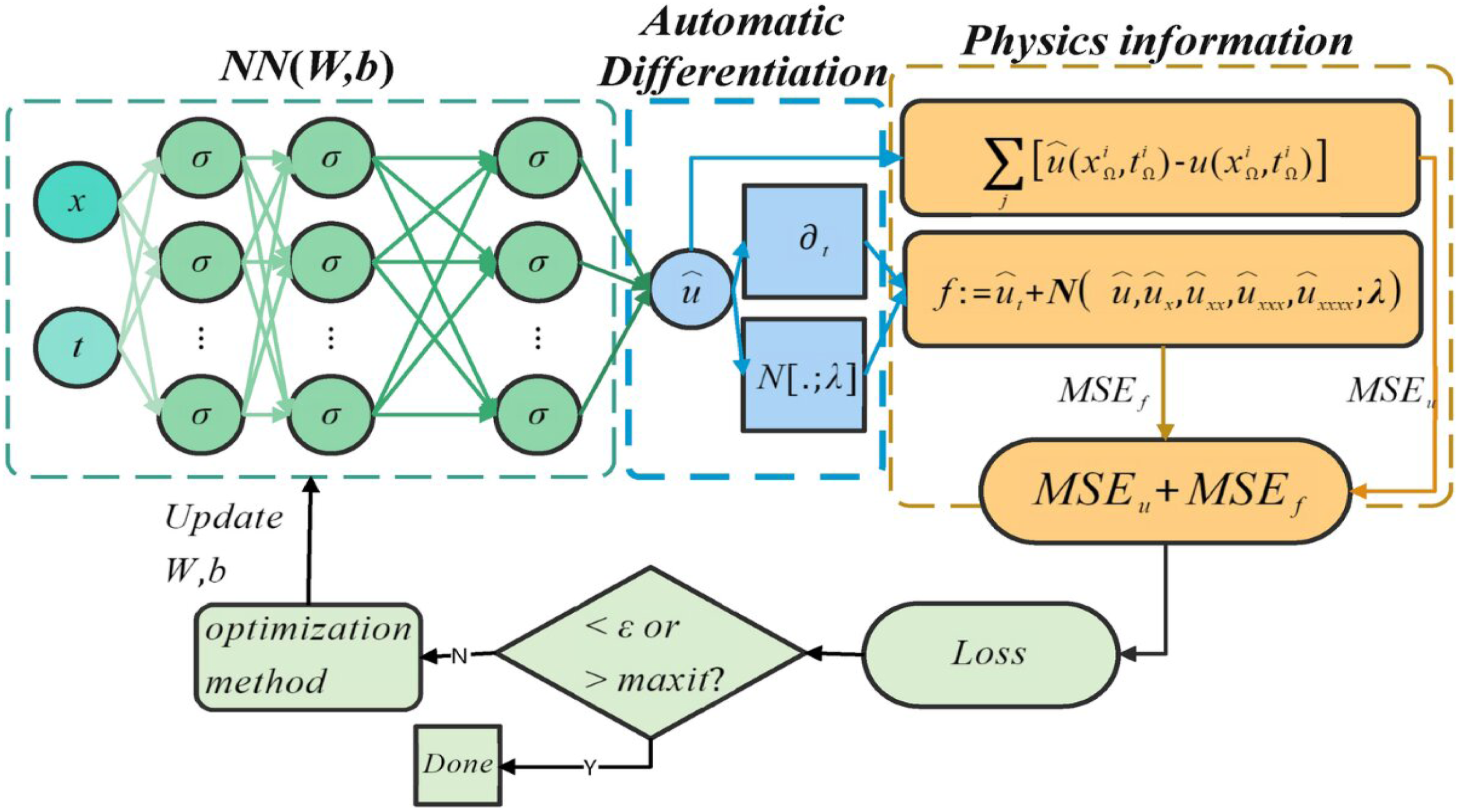

We shall represent g(x, t) as the expression on the left of the equation above.

g ≔ v_{t} + ℵ [v],

(14)

Then latter v(x, t) is estimated with the help of a deep neural network. According to this assumption, and the result of the above equation in the PINN g(x, t).³⁸ It is defined by applying the chain rule of differentiation to the composition of functions through automatic differentiation (is a computational method of computing derivatives or gradients of functions written in the form of code). It is identically structured as the neural network which models v(x, t), but with alternate activation functions due to the effect of the differential operator ℵ on g(x, t). Under the training, the function g(x, t) can be trained with the loss of mean squared error.

M S E = M S E_{v} + M S E_{g},

(15)

where,

M S E_{v} = \frac{1}{N_{v}} Σ_{i = 1}^{N_{v}} | v (t_{v}^{i} - v^{i}) |^{2},

(16)

and

M S E_{g} = \frac{1}{N_{g}} Σ_{i = 1}^{N_{g}} | g (t_{g}^{i}, x_{g}^{i}) |^{2} .

(17)

In this case, ${(t_{v}^{i}, x_{v}^{i}, v^{i})}_{i = 1}^{N_{v}}$ is the initial and boundary condition training data of v(x, t) and ${(t_{g}^{i}, x_{g}^{i})}_{i = 1}^{N_{g}}$ is the points of collocation of g(x, t). The loss MSE_v corresponds to the initial and the boundary data whereas, MSE_g guarantees the structure which may be derived by equation at a finite set of collocation points. Although the ideas of constraining physics laws have been discussed previously in the literature on neural networks, the current study makes use of the modern computational to apply the concepts to more complex dynamic problems which are defined by NLPDE.

2.2. gPINN

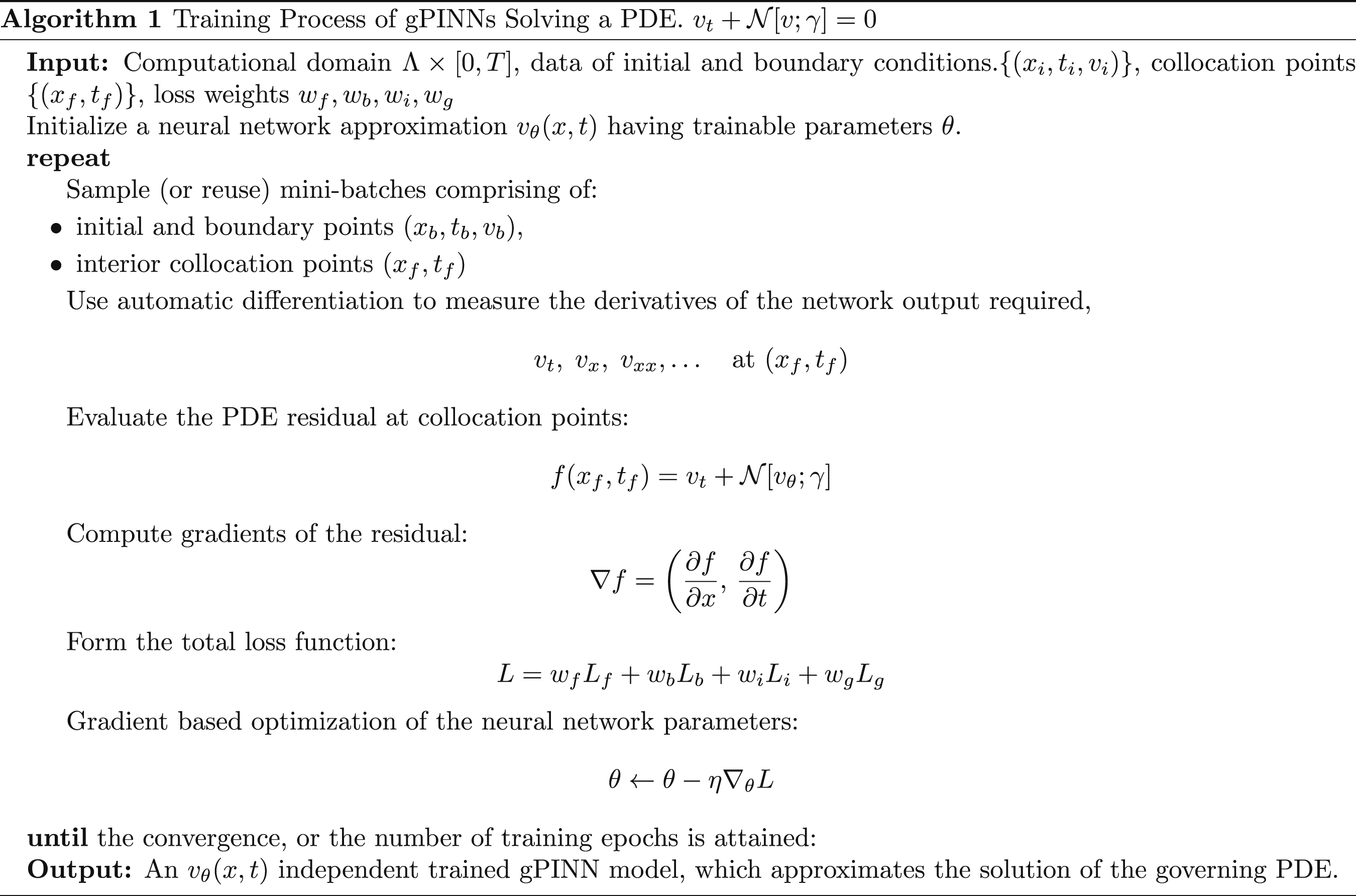
The residual f of PINNs is the only thing we demand, as on the points where f(x) should be zero, the derivative of f(x) should be zero as well. ³⁹ In gPINN we make the assumption that the exact solution of the PDE is smooth enough to permit the existence of the gradient of the PDE residual,∇f(x) (Figure 2). Then, we propose gradient-enhanced PINNs, which is to make sure that the derivatives of the PDE residual are also equal to zero. i. e

\nabla f (x) = (\frac{\partial f}{\partial x_{1}}, \frac{\partial f}{\partial x_{2}}, \frac{\partial f}{\partial x_{3}}, \dots, \frac{\partial f}{\partial x_{n}}) = 0, x \in Λ

(18)

Figure 2.

gPINN algorithm.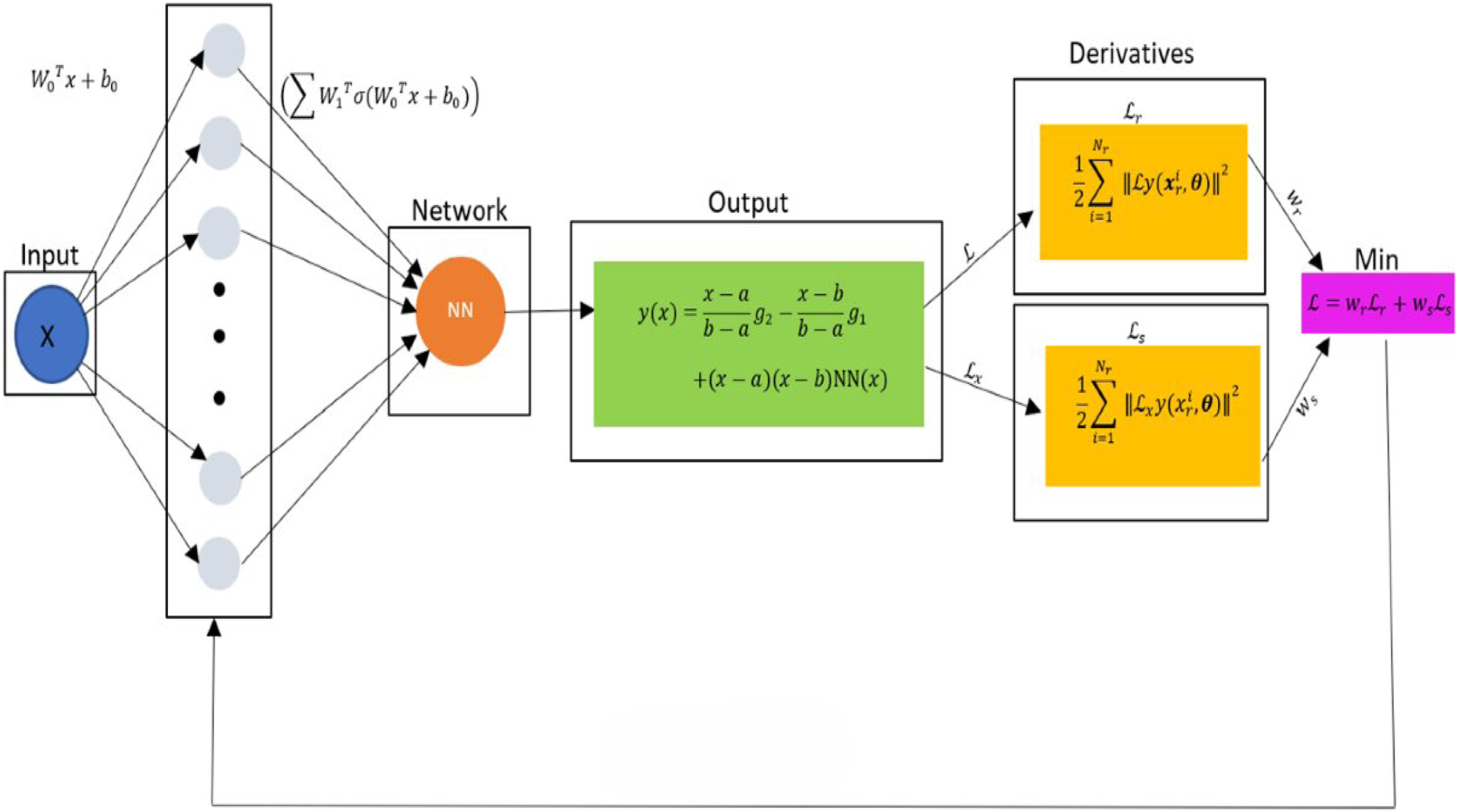

The overall gPINN loss function can be formulated as below:

L_{gPINN} = w_{f} L_{f} + w_{b} L_{b} + w_{i} L_{i} + Σ_{i = 1}^{n} w_{g_{i}} L_{g_{i}} (ψ; T_{g_{i}}),

(19)

where the derivative loss in respect of x_i.

L_{g_{i}} (ψ; T_{g_{i}}) = \frac{1}{| T_{g_{i}} |} Σ_{x \in T_{g_{i}}} | \frac{\partial f}{\partial x_{i}} |^{2},

(20)

The derivative ∂f/∂x_i represents a collection of residual points denoted by $T_{g_{i}}$ . In this study we decide that $T_{g_{i}}$ = T_f and that T_f and $T_{g_{i}} (i = 1, \dots, d)$ may not be equal. The weights that we have chosen in this investigation are $w_{g_{1}} = w_{g_{2}} = \dots = w_{g_{d}}$ . The ideal value of the weight is determined with the use of grid search. The neural network u(x; ψ) that we are trying to approximate the solution u(x) is built with a trainable factor ψ.

2.3. XPINN

In extended physics informed neural networks there is no necessity to determine the normal direction, to implement normal flux continuity condition. This greatly simplifies the algorithm, especially when using large scale problems with the complicated domains, too, and when using moving interface problems.

In this regard, the computational domain is broken to N_sd number of non-overlapping regular/irregular sub-domains. The neural network output of the m^th sub-domain in the XPINN model is represented by⁴⁰ (Figure 3).

v_{g_{m}} (x) = N^{L} (x; g_{m}) \in Φ_{m}, m = 1,2,3, \dots, N_{s d}

(21)

where N^L refers to the neurons of L layers. Φ_m represents a set of weights and biases and slopes. N_sd number of regular/irregular sub-domains that are not overlapping.

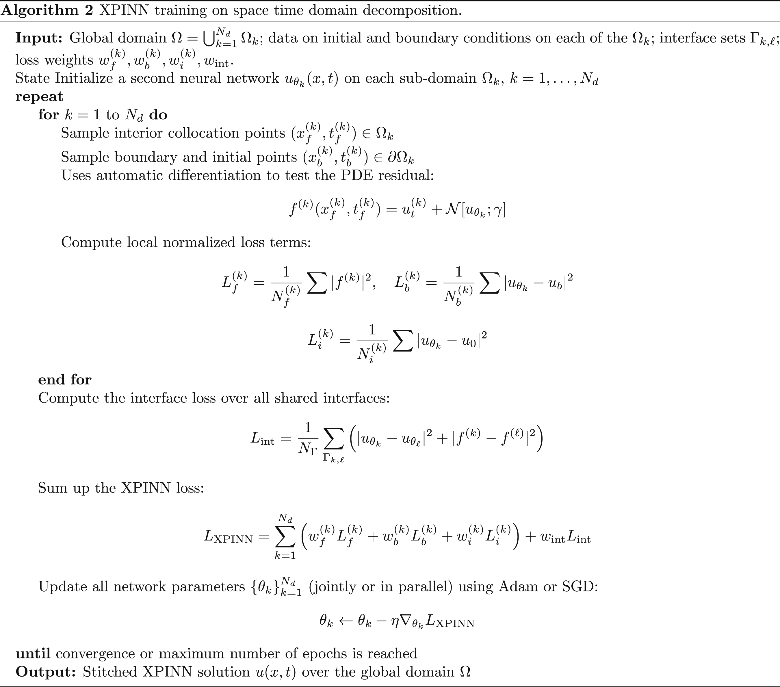
Figure 3.

XPINN algorithm.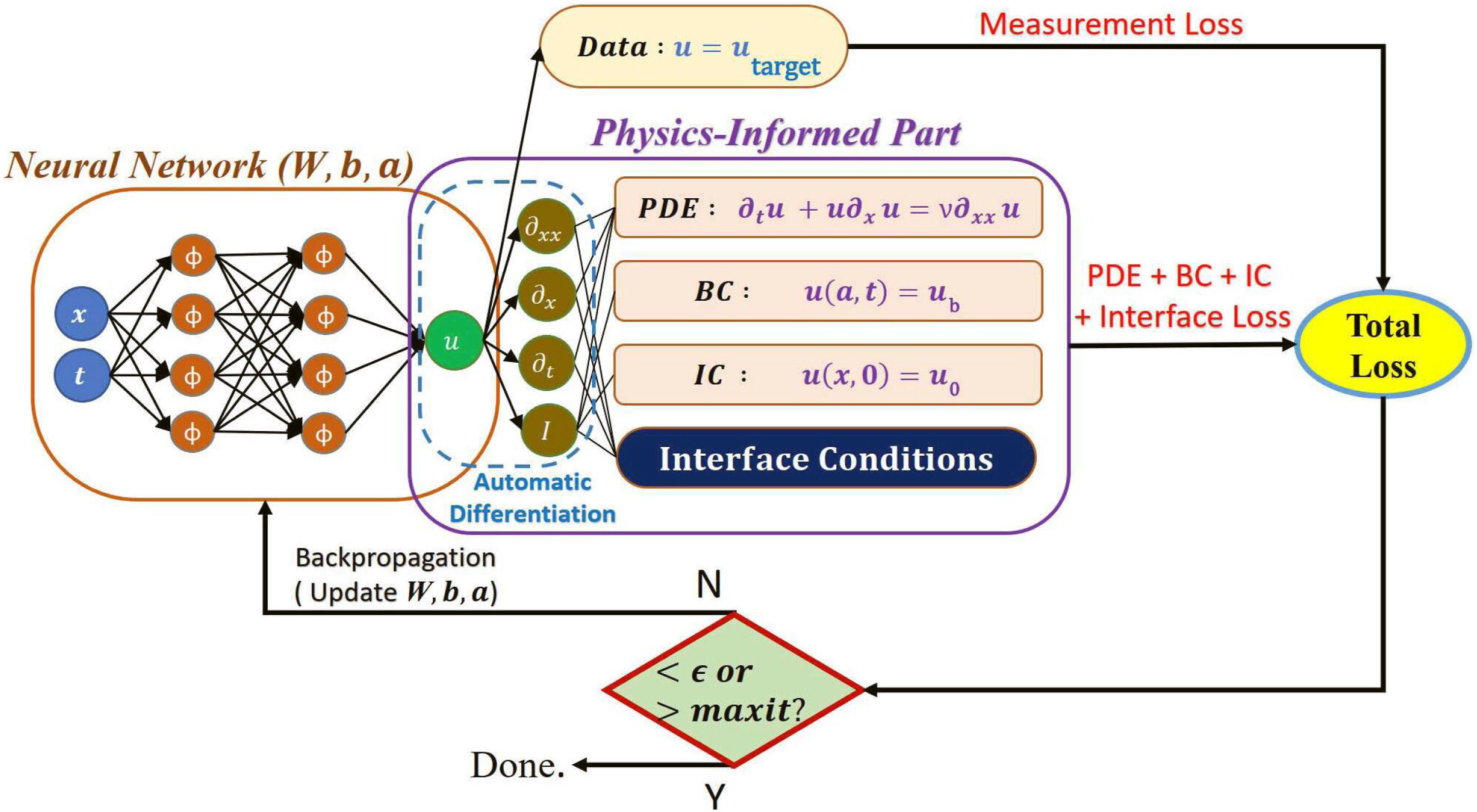

The resultant outcome is by,

v_{g_{m}} (x) = Σ_{m = 1}^{N_{s d}} v_{g_{m}} \cdot l_{Φ_{m}} (x) .

(22)

and where the indicator function of $l_{Φ_{m}}$ is given as

l_{Φ_{m}} (x) = \{\begin{cases} 0 & if x \notin Φ_{m}, \\ 1 & if x \in Φ_{m} \ Common interface in Φ_{m}, \\ \frac{1}{S} & if x \in Common interface in Φ_{m} . \end{cases}

(23)

where S denote the number of sub-domains that are intersecting on the common interface.

The overall loss of XPINN can be written in the following way:

L_{XPINN} = w_{v_{m}} M S E_{v_{m}} + w_{f_{m}} M S E_{F_{m}} + w_{v_{avg}} M S E_{v_{avg}} + w_{R} M S E_{R},

(24)

The mean square error of each term is provided by,

{M S E}_{v_{m}} = \frac{1}{N_{v_{m}}} Σ_{i = 1}^{N_{v_{m}}} | v^{i} - v_{Φ_{m}} {(x_{v_{m}})}^{i}) |^{2},

(25)

and

M S E_{F_{m}} = \frac{1}{N_{F_{m}}} Σ_{i = 1}^{N_{F_{m}}} | F_{Φ_{m}} (x_{F_{m}}^{i}) |^{2} .

(26)

M S E_{v_{avg}} = Σ_{\forall m^{+}} \frac{1}{N_{I_{m}}} Σ_{i = 1}^{N_{I_{m}}} | v_{Ψ_{m}} (x_{I_{m}}^{i}) - [v_{Φ_{m}} (x_{I_{m}}^{i})] |^{2} .

(27)

M S E_{R} = Σ_{\forall m^{+}} \frac{1}{N_{I_{m}}} Σ_{i = 1}^{N_{I_{m}}} | F_{Ψ_{m}} (x_{I_{m}}^{i}) - [F_{Φ_{m}^{+}} (x_{I_{m}}^{i})] |^{2} .

(28)

where

M S E_{v_{m}}

and

M S E_{F_{m}}

are the terms of data mismatch dissipation and loss of residual and F = F_q is the residual of the governing PDEs in the m^th sub-domain. The MSE_R is the continuity property of the shared interface that is presented by two neural networks in sub-domains q and q+ respectively; the + superscript on q is the neighbouring sub-domain(s). To normalise the impact of each of the components of the loss, the weighting coefficients were

w_{v_{m}}

w_{f_{m}}

w_{v_{avg}}

and w_R added, especially since the effects of the PDE residual and boundary/initial errors may vary by several orders of magnitude. Both terms MSE_R and

M S E_{v_{avg}}

are defined to all neighboring sub-domain(s) q+ that is the summation in the expression.

3. Mathematical analysis

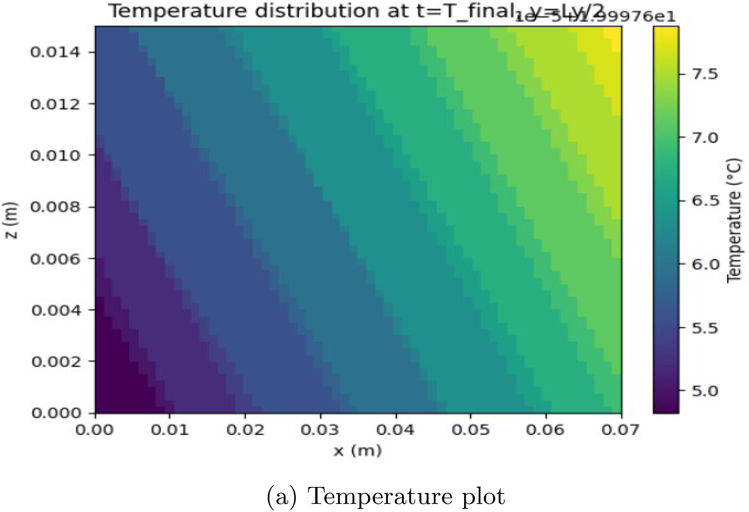
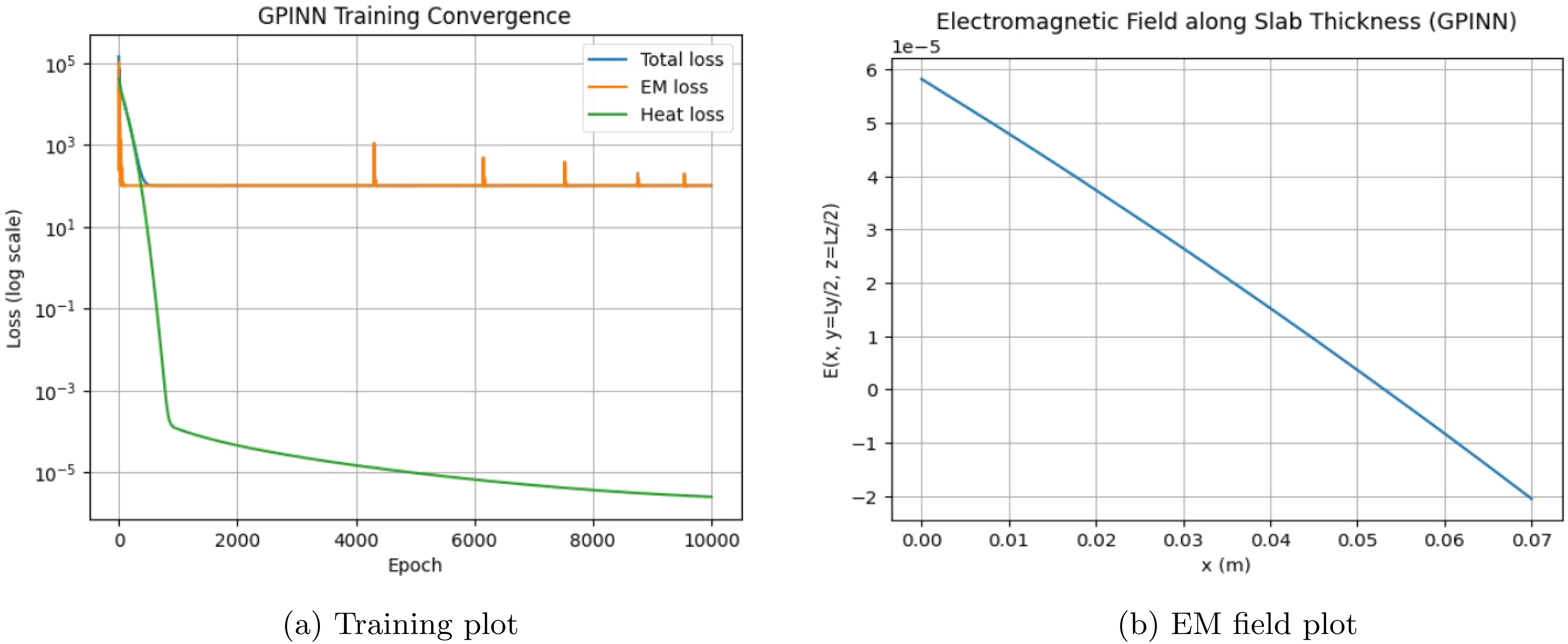
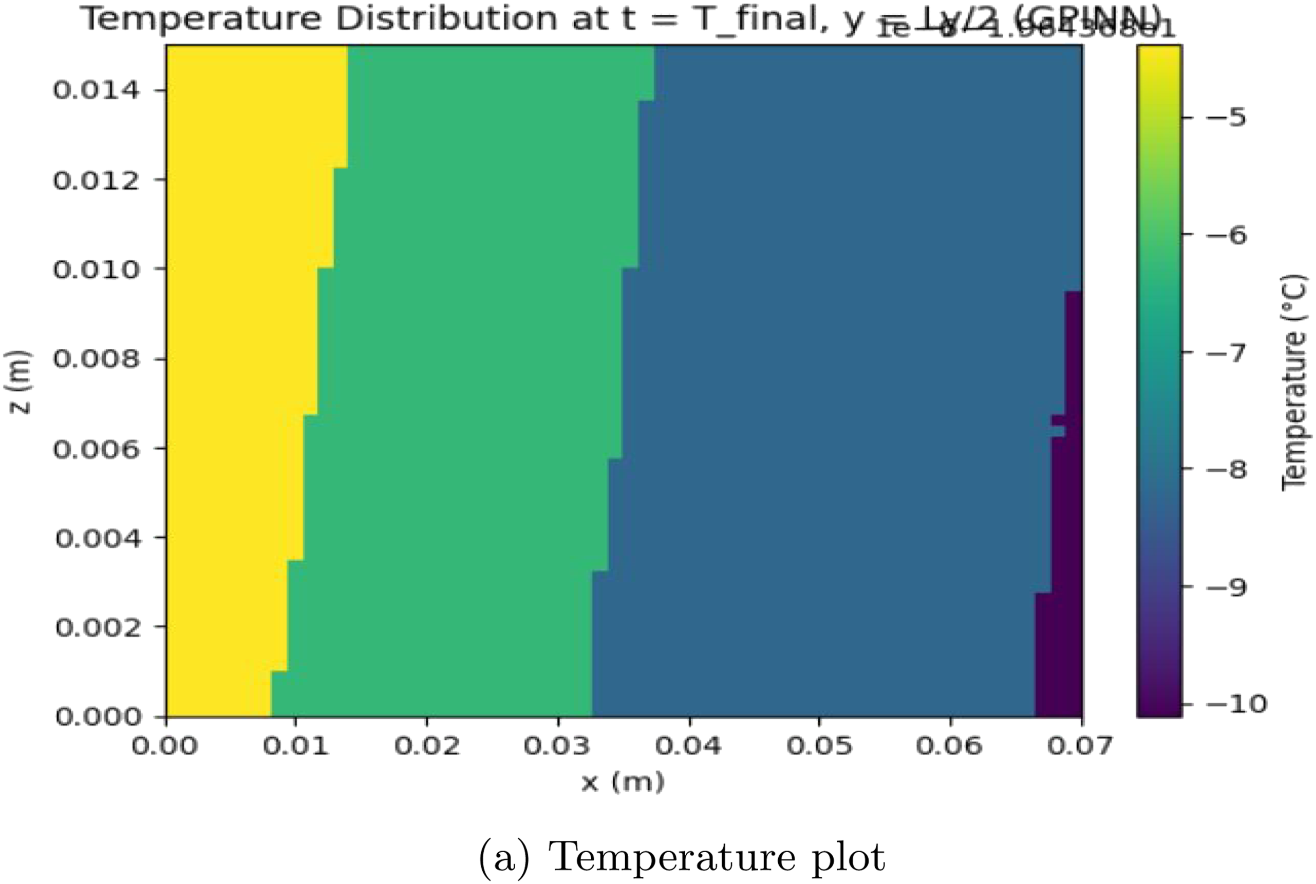
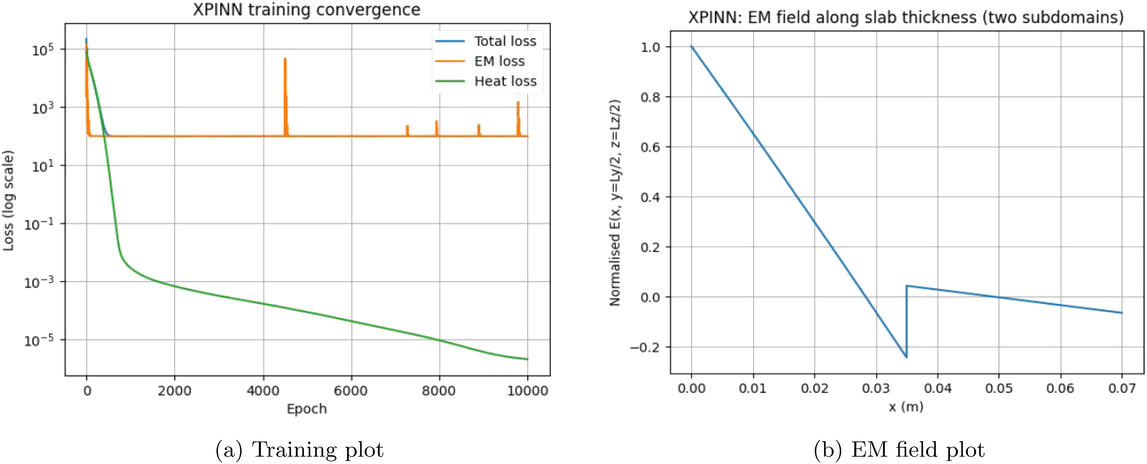
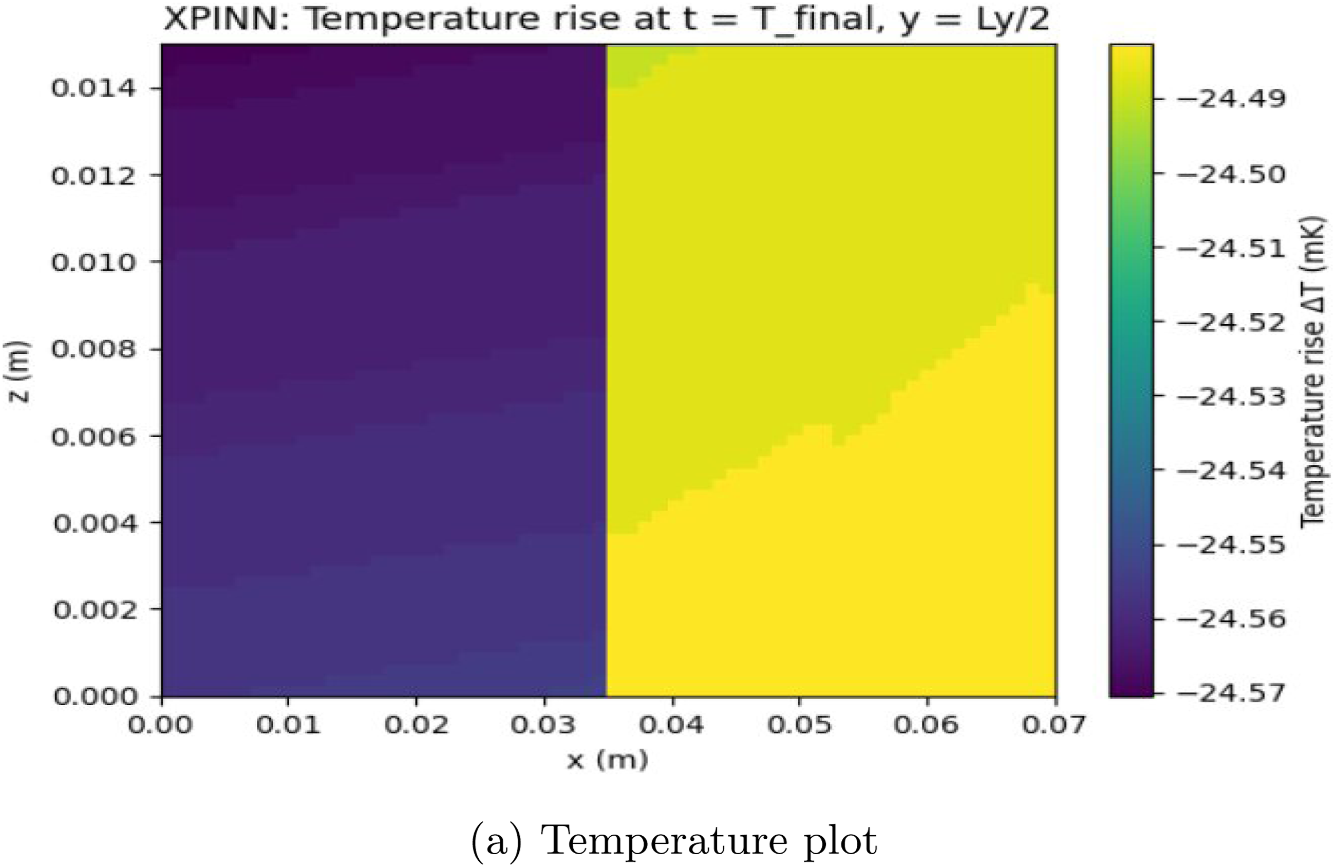
This section will develop the proposed physics-informed framework to tackle nonlinear electromagnetic heating in an environment with temperature-dependent properties. The formulation allows a consistent application of PINN, gPINN, and XPINN to a common framework to enable a systematic comparison of their performance on nonlinear source-driven problems (Figures 4–9).

Figure 4.

(a). The training convergence history of the PINN in which total loss, electromagnetic loss, and heat equation loss have been plotted on a logarithmic scale. The loss of the heat equation decreases rapidly at the first stage of training and after that, converges steadily. The electromagnetic loss is almost constant and it implies that the electromagnetic constraint is enforced in a stable manner. (b). The distribution of electromagnetic field perpendicular through the thickness of the slab across the mid-plane contain smooth spatial variation in the direction of propagation. This field distribution dictates the spatial variation of the volumetric heat generation of electromagnetic in the slab.

Figure 5.

The distribution of the temperature predicted at the end of time, as the slab thickness increases, is gradual, which agrees with the pattern of power absorption of electromagnetism. The extended smooth temperature contours show that the PINN solution is able to meet the governing physics without the introduction of numerical oscillations.

Figure 6.

(a). The history of the convergence of training of the gPINN depicts the history of the total loss, electromagnetic loss and heat equation loss on a logarithmic scale. The reduction in the heat equation loss is high at the beginning of the training, and then, the convergence is smooth and stable. The loss in the heat equation converges more uniformly in comparison with the PINN case as a result of the inclusion of gradient information whereas the electromagnetic loss is almost constant, meaning the electromagnetic constraint has been enforced steadily. (b). The distribution of electromagnetic field across the slab thickness at the mid–plane has smooth spatial variation along the direction of propagation. The field profile will be in line with the projected electromagnetic action within the dielectric slab and will identify the spatial field of the electromagnetic heat source.

Figure 7.

The expected temperature distribution at the final time demonstrates more distinct spatial differentiation of levels of temperature along the slab thickness. Temperature contours are smoother and more homogenous than the PINN ones, which means that the temperature gradients are better resolved, and the solution is more stable.

Figure 8.

(a). The XPINN training convergence history demonstrates how the total loss, electromagnetic loss as well as the heat equation loss changes with time on a logarithmic scale. The loss of the heat equation is reduced quickly during the preliminary phase of training, then it stabilizes on the smaller values. The electromagnetic loss is almost constant over the course of training, which shows that there is a consistent application of the electromagnetic constraint to subdomains. (b). Electromagnetic field distribution along the slab thickness at the mid–plane exhibits a piecewise smooth variation which is due to the two subdomains. The field profile at the interface is continuous, which proves that the interface conditions are correctly applied in the XPINN and the electromagnetic behavior within the slab is as desired.

Figure 9.

It is observed that the distribution of predicted temperature at the last time has smooth spatial variation on the whole domain which includes the subdomain interface. The temperature figures are revealing uniform gradients in the slab thickness devoid of observed discontinuities, which indicated sufficient coupling between subdomains and correctly resolving the electromagnetic heating process.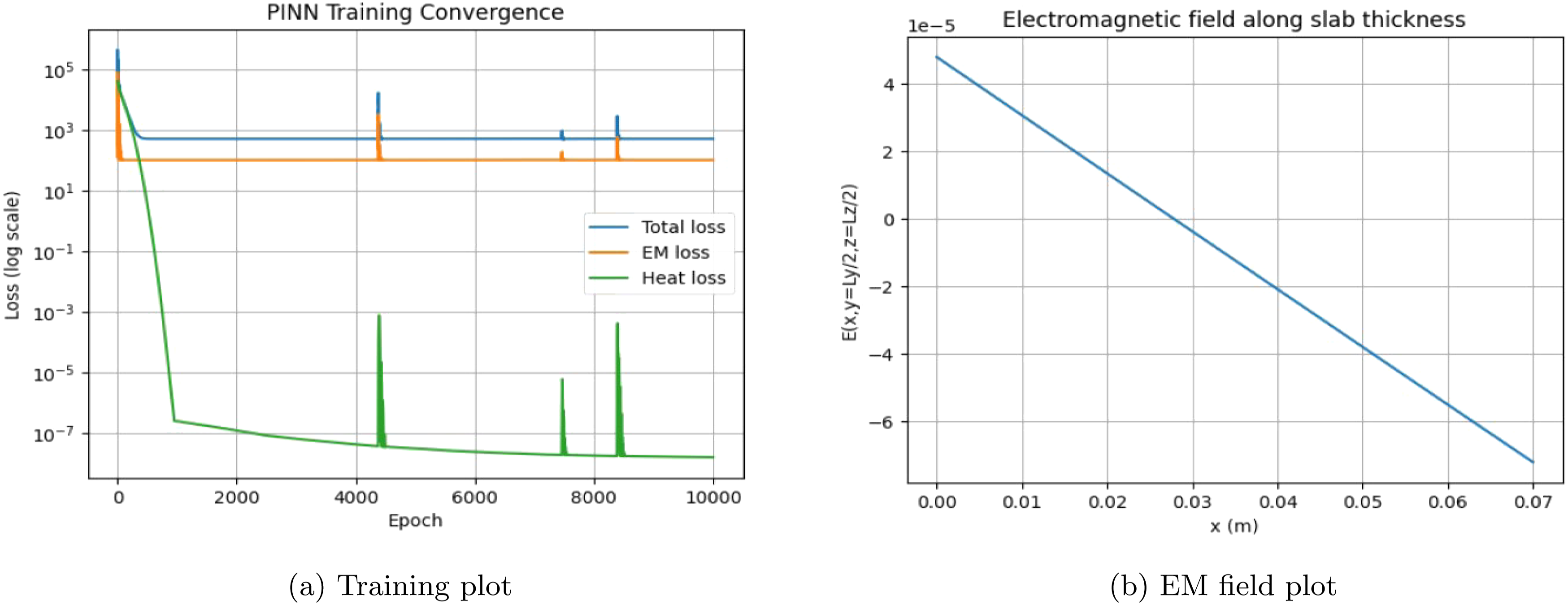

3.1. PINN analysis of electromagnetic heating

It provides a model of a coupled electromagnetic thermal problem of radio-frequency (RF) heating of a biological tissue slab modeled with a PINN. The system has an electromagnetic wave equation combined with a heat diffusion equation with the dielectric losses producing heat. The effect of temperature-dependent material properties results in nonlinear feedback between the electromagnetic field and thermal behavior and account for effects of heat transfer across boundaries.

3.1.1. Architecture of neural networks

3.1.1.1. Electric field network (net_E)

• Input: Spatial coordinates (x, y, z)

• Output: Electric field magnitude E(x, y, z)

• Architecture: 5 hidden layers, 80 neurons per layer, tanh activation

3.1.1.2. Temperature network (net_T)

• Input: Spatial and temporal coordinates (x, y, z, t)

• Output: Temperature T(x, y, z, t)

• Architecture: 4 hidden layers, 64 neurons per layer, tanh activation

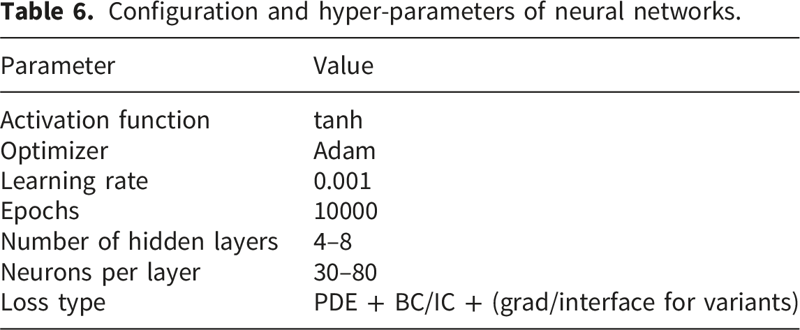
The neural networks employed in the current study are fully connected feedforward networks with tanh activation functions. The electromagnetic field and temperature prediction are done separately in different networks. The electromagnetic network uses spatial coordinates as input whereas the thermal network uses both spatial and time coordinates. Every network is trained with the Adam optimizer with the same learning rates, so that the results are consistent across variants of PINN.

3.1.2. Physics constraints implementation

Electromagnetic Equation: The electric field satisfies an equation of the type of a Helmholtz, with the Laplacian of the field balanced by a coefficient depending on the temperature:

\nabla^{2} E + (ν^{2} + σ (T)) E = 0,

(29)

Heat Transfer Equation: The temperature dynamics is a transient equation of heat diffusion that has source term due to absorption of electromagnetic energy:

\frac{\partial T}{\partial t} = α \nabla^{2} T + S,

(30)

and the heating source term is the Joule heating.

S = C_{source} E^{2}, C_{source} = \frac{0.5 ω ε_{0} ε^{″}}{ρ c_{p}} .

The electro magnetic thermal interaction is added in the current formulation by including a temperature dependent heat generation term. A simplified or quasi-static assumption is made regarding the distribution of electric fields, and its effect is added to the heat equation, in the form of the source term. This method is ideal in capturing the prevailing coupling between temperature evolution and electromagnetic energy absorption, without the computational complexity of a fully coupled solution of the Maxwell equations.

3.1.2.1. Boundary and initial conditions

• Electromagnetic condition: Electric field is stipulated on the excitation boundary, with E(x = 0) = E₀

• The thermal condition is set at an even temperature all over the domain as T(x, y, z, t = 0) = T₀.

The loss function imposes the soft constraints of the boundary and initial conditions. In the training, the network reduces the PDE residual, as well as the difference between the learned solution and the boundary and initial conditions that are prescribed, so that the governing physical laws are met.

Temperature-Dependent Property: The dielectric loss is linearly dependent with temperature:

σ (T) = ε_{0} ε^{″} (T) [1 + β_{σ} (T - T_{0})] .

(31)

Such a dependence brings about nonlinear interaction between the electromagnetic and thermal fields.

3.1.3. Training strategy

Collocation Points:

• Electromagnetic field: 12 × 10 × 10 = 1200 spatial points.

• Heat domain: 20 × 12 × 10 × 10 = 24000 space-time points.

• Initial condition: 3-D spatial grid at t = 0.

Loss Formulation: The overall loss of training is composed of a weighted sum of the residuals of the governing PDE and the boundary/initial condition errors.

Loss weighting strategy: To give importance to proper prediction of electromagnetic fields, the weight of EM residual is multiplied by a factor five to that of the thermal residual.

Optimization Scheme: The Adam optimizer is employed with a learning rate of 10⁻³ through 10000 iterations of training.

The overall loss is determined as a weighted mean of the PDE residual, boundary condition loss, and the initial condition loss. The set of weighting coefficients is chosen to balance the contribution of each term and stable convergence in the course of training.

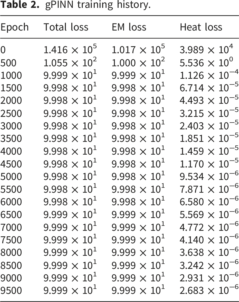
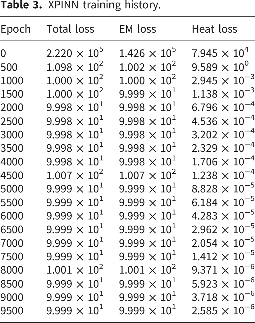
Multi-physics problems can have imbalance in the various components of the loss during training because they do not necessarily scale the same way. This may cause more gradual convergence of some residual values than others. In the current analysis, it can be seen that electromagnetic residual converges slower than thermal residual meaning that a larger component of thermal loss dominates during optimization.

3.1.4. Simulation and physical parameters

• A slab of size (7 cm x 4 cm x 1.5cm) which is rectangular.

• The medium is biological tissue whose density ρ = 1047.89 kg/m³ and specific heat capacity c_p = 3589.4 J/(kg ⋅ K) values are known.

• A radio frequency (RF) generator with frequency 40 MHz is used and the starting amplitude of the electric field is E₀ = 1 V/m.

• A model of heat loss to the environment is represented by a convective boundary condition, where the heat transfer coefficient is h = 10 W/(m² ⋅ K), and it is implicitly considered in the PINN framework.

• The heating of the material takes place within 75 seconds.

3.1.5. Visualization and outputs

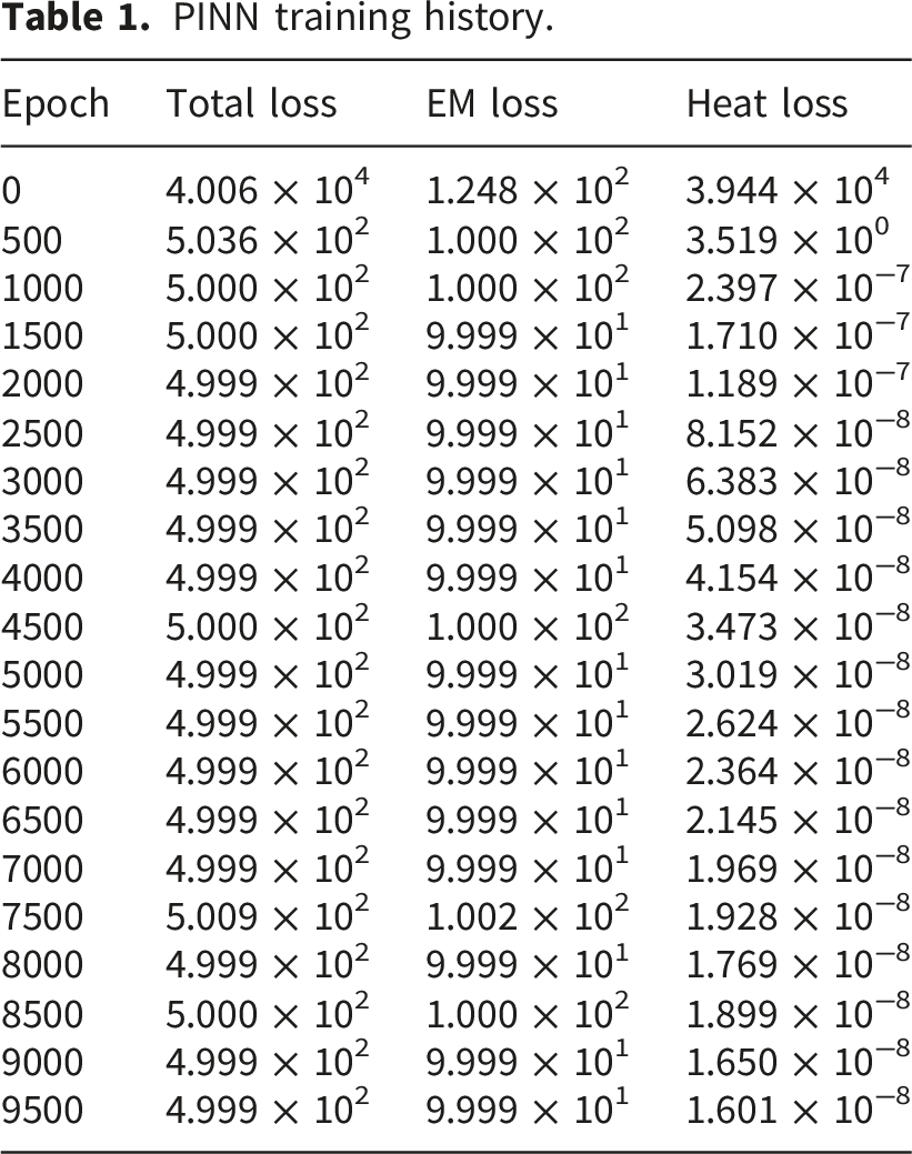
In this problem the model generates Root-mean-square residual of electromagnetic equation at the end of training is 1.101 × 10⁻¹. where as the root-mean-square residual of the heat equation is 2.788 × 10⁻⁵. The values show that the PINN is a good solution of the heat equation, and the electromagnetic constraint is still good (Tables 1–4).

Table 1.

PINN training history.

Epoch	Total loss	EM loss	Heat loss
0	4.006 × 10⁴	1.248 × 10²	3.944 × 10⁴
500	5.036 × 10²	1.000 × 10²	3.519 × 10⁰
1000	5.000 × 10²	1.000 × 10²	2.397 × 10⁻⁷
1500	5.000 × 10²	9.999 × 10¹	1.710 × 10⁻⁷
2000	4.999 × 10²	9.999 × 10¹	1.189 × 10⁻⁷
2500	4.999 × 10²	9.999 × 10¹	8.152 × 10⁻⁸
3000	4.999 × 10²	9.999 × 10¹	6.383 × 10⁻⁸
3500	4.999 × 10²	9.999 × 10¹	5.098 × 10⁻⁸
4000	4.999 × 10²	9.999 × 10¹	4.154 × 10⁻⁸
4500	5.000 × 10²	1.000 × 10²	3.473 × 10⁻⁸
5000	4.999 × 10²	9.999 × 10¹	3.019 × 10⁻⁸
5500	4.999 × 10²	9.999 × 10¹	2.624 × 10⁻⁸
6000	4.999 × 10²	9.999 × 10¹	2.364 × 10⁻⁸
6500	4.999 × 10²	9.999 × 10¹	2.145 × 10⁻⁸
7000	4.999 × 10²	9.999 × 10¹	1.969 × 10⁻⁸
7500	5.009 × 10²	1.002 × 10²	1.928 × 10⁻⁸
8000	4.999 × 10²	9.999 × 10¹	1.769 × 10⁻⁸
8500	5.000 × 10²	1.000 × 10²	1.899 × 10⁻⁸
9000	4.999 × 10²	9.999 × 10¹	1.650 × 10⁻⁸
9500	4.999 × 10²	9.999 × 10¹	1.601 × 10⁻⁸

Table 2.

gPINN training history.

Epoch	Total loss	EM loss	Heat loss
0	1.416 × 10⁵	1.017 × 10⁵	3.989 × 10⁴
500	1.055 × 10²	1.000 × 10²	5.536 × 10⁰
1000	9.999 × 10¹	9.999 × 10¹	1.126 × 10⁻⁴
1500	9.998 × 10¹	9.998 × 10¹	6.714 × 10⁻⁵
2000	9.998 × 10¹	9.998 × 10¹	4.493 × 10⁻⁵
2500	9.998 × 10¹	9.998 × 10¹	3.215 × 10⁻⁵
3000	9.998 × 10¹	9.998 × 10¹	2.403 × 10⁻⁵
3500	9.998 × 10¹	9.998 × 10¹	1.851 × 10⁻⁵
4000	9.998 × 10¹	9.998 × 10¹	1.459 × 10⁻⁵
4500	9.998 × 10¹	9.998 × 10¹	1.170 × 10⁻⁵
5000	9.998 × 10¹	9.998 × 10¹	9.534 × 10⁻⁶
5500	9.998 × 10¹	9.998 × 10¹	7.871 × 10⁻⁶
6000	9.998 × 10¹	9.998 × 10¹	6.580 × 10⁻⁶
6500	9.999 × 10¹	9.999 × 10¹	5.569 × 10⁻⁶
7000	9.999 × 10¹	9.999 × 10¹	4.772 × 10⁻⁶
7500	9.999 × 10¹	9.999 × 10¹	4.140 × 10⁻⁶
8000	9.999 × 10¹	9.999 × 10¹	3.638 × 10⁻⁶
8500	9.999 × 10¹	9.999 × 10¹	3.242 × 10⁻⁶
9000	9.999 × 10¹	9.999 × 10¹	2.931 × 10⁻⁶
9500	9.999 × 10¹	9.999 × 10¹	2.683 × 10⁻⁶

Table 3.

XPINN training history.

Epoch	Total loss	EM loss	Heat loss
0	2.220 × 10⁵	1.426 × 10⁵	7.945 × 10⁴
500	1.098 × 10²	1.002 × 10²	9.589 × 10⁰
1000	1.000 × 10²	1.000 × 10²	2.945 × 10⁻³
1500	1.000 × 10²	9.999 × 10¹	1.138 × 10⁻³
2000	9.998 × 10¹	9.998 × 10¹	6.796 × 10⁻⁴
2500	9.998 × 10¹	9.998 × 10¹	4.536 × 10⁻⁴
3000	9.998 × 10¹	9.998 × 10¹	3.202 × 10⁻⁴
3500	9.998 × 10¹	9.998 × 10¹	2.329 × 10⁻⁴
4000	9.998 × 10¹	9.998 × 10¹	1.706 × 10⁻⁴
4500	1.007 × 10²	1.007 × 10²	1.238 × 10⁻⁴
5000	9.999 × 10¹	9.999 × 10¹	8.828 × 10⁻⁵
5500	9.999 × 10¹	9.999 × 10¹	6.184 × 10⁻⁵
6000	9.999 × 10¹	9.999 × 10¹	4.283 × 10⁻⁵
6500	9.999 × 10¹	9.999 × 10¹	2.962 × 10⁻⁵
7000	9.999 × 10¹	9.999 × 10¹	2.054 × 10⁻⁵
7500	9.999 × 10¹	9.999 × 10¹	1.412 × 10⁻⁵
8000	1.001 × 10²	1.001 × 10²	9.371 × 10⁻⁶
8500	9.999 × 10¹	9.999 × 10¹	5.923 × 10⁻⁶
9000	9.999 × 10¹	9.999 × 10¹	3.718 × 10⁻⁶
9500	9.999 × 10¹	9.999 × 10¹	2.585 × 10⁻⁶

Table 4.

Comparison of PINN, gPINN, and XPINN for microwave heating simulation.

Aspect	PINN	gPINN	XPINN
Core idea	Single network enforcing PDE residuals	PINN with gradient regularization of residuals	Domain decomposition with multiple networks
Network Architecture	2 networks(EM + Thermal)	2 networks(EM + Thermal)	4 networks(2 EM + 2 Thermal)
Loss Function	PDE residuals + BC/IC penalties	PDE residuals + gradient penalties + BC/IC	PDE residuals + interface continuity + BC/IC
Regularization	Adaptive weighting (λ_bc = 10², λ_ic = 10²)	Gradient penalties (λ_grad = 10⁻¹) + BC/IC	Interface conditions (λ_int = 10²)
Domain Treatment	Single continuous domain [0, L_x]	Single continuous domain [0, L_x]	Two subdomains split at x = L_x/2
Coupling Approach	Decoupled one-way	Decoupled one-way	Decoupled one-way
Interface Handling	Not applicable	Not applicable	C¹ continuity (field and gradient matching)
Computational Cost	Lowest	Medium	Highest
Training Time	Fastest	Medium (extra gradient computations)	Slowest (multiple networks + interface losses)
Parallelization	Limited	Limited	High potential
Accuracy Metric	RMS residuals: EM (10⁻²), Heat (10⁻³)	RMS residuals: EM (10⁻²), Heat (10⁻³)	RMS residuals: EM (10⁻²), Heat (10⁻³)
Convergence	Standard optimization	Smoother due to gradient regularization	May require careful interface tuning
Scalability	Limited by single network capacity	Limited by single network capacity	Better for large and complex domains
Flexibility	Fixed architecture	Fixed architecture	Different architectures per subdomain possible
Implementation Complexity	Simplest	Medium (gradient computation overhead)	Most complex (interface management)
Best For	Standard problems, moderate accuracy	Problems requiring smoother solutions	Heterogeneous domains and parallel computing
Key Innovation	Physics enforcement via residuals	Enforcing residual smoothness via gradients	Domain decomposition with continuity constraints
Physical Consistency	PDE satisfaction only	PDE + gradient consistency	PDE + interface continuity + subdomain coupling

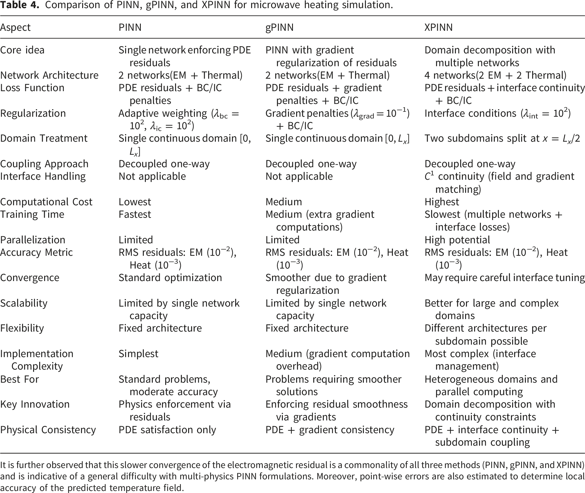
It is further observed that this slower convergence of the electromagnetic residual is a commonality of all three methods (PINN, gPINN, and XPINN) and is indicative of a general difficulty with multi-physics PINN formulations. Moreover, point-wise errors are also estimated to determine local accuracy of the predicted temperature field.

3.2. gPINN on electromagnetic heating problems

The gPINN model is a framework that adds extra gradient-based residual terms to the loss. These terms not only impose consistency on the governing equation, but also on its spatial derivatives, resulting in better convergence and increased accuracy. This method is especially useful in the sharp temperature gradient and local changes of electromagnetic heating issues. In the study, a simplified electromagnetic heating formulation is considered in which the electric field is considered separately and it adds to the heat equation as the source term with the use of the gPINN model.

3.2.1. Decoupled system of simplified physics

• Electromagnetic Equation: ∇²E + ν²E = 0, (no temperature-dependent).

• Heat Equation: ∂T/∂t − α∇²T − C_source|E|² = 0

• Decoupling Assumption: EM field is decoupled, and it is used as source to heat equation.

This use of the term decoupled means the simplified action of the electromagnetic field, although the thermal equation is nonlinear owing to the temperature-dependent source term. This equation is compatible with the most commonly used electromagnetic heating models, where the heat generation term is the dominant coupling.

3.2.2. Neural network structure

• net_E: 3D → 1D fully connected neural network (64 width, 4 depth, tanh activation)

• net_T: 4D → 1D fully connected neural network (identical architecture)

Both networks are updated concurrently using the Adam optimizer.

3.2.3. Gradient-enhanced loss

In addition to the reduction of PDE residuals, the gradients of the residuals are also added to the loss function:

L = MSE (R) + λ MSE (\nabla R),

(32)

where

R

represents the residual of the governing equation. This is an improvement that enhances convergence behavior and improves derivative predictions accuracy.

3.2.4. Training strategy

3.2.4.1. Collocation sampling

• Electromagnetic domain: Helmholtz steady state equation is applied on a grid of 10 × 10 × 10 grid points.

• Thermal domain:The space time domain of the transient heat equation has a four dimensional grid of 10 × 10 × 10 × 20 points.

3.2.4.2. Loss composition

The training objective will be made up of the following elements:

1. Remaining electromagnetic PDE loss,

2. Sloping drop of the electromagnetic residual,

3. Boundary constraint enforcing E(0, 0, 0) = 1.0,

4. Thermal PDE residual loss,

5. Stepping loss of the thermal residual,

6. Initial condition constraint T(x, y, z, 0) = 20°C.

3.2.4.3. Training parameters

• Learning rate: 1 × 10⁻³,

• Number of epochs: 10, 000,

• Total simulated time: 75 s,

• Slab dimensions (size): 70 × 40 × 15 mm.

3.2.5. Visualization and outputs

The root-mean-square residual of the electromagnetic equation after the training is at the end of training. 1.157 × 10⁻¹ Whereas the root-mean-square residual of the heat equation is 1.536 × 10⁻³. These findings indicate that gPINN methodology gives better convergence properties and the association between electromagnetic and thermal constraints is stable.

3.3. XPINN on electromagnetic heating problems

The XPINN model breaks down the computational space into several non-overlapping sub spaces where the individual neural networks are assigned to the different regions. The loss function contains interface continuity conditions which guarantee consistency of the solution and its gradients at subdomain boundaries. It is a domain decomposition approach which enhances convergence and facilitates the effective modeling of local nonlinear behavior in electromagnetic heating problems.

3.3.1. Domain decomposition

The whole point is to subdivide the 7 cm thick tissue area into two distinct parts:

• Left subdomain (0–3.5 cm): The $n e t_E 1$ can be used to predict the electromagnetic field of a body and the $n e t_T 1$ can be used to predict the temperature of a body.

• Right subdomain (3.5–7 cm): The processing of the electromagnetic field occurs through $n e t_E 2$ and the temperature is calculated through $n e t_T 2$ .

3.3.2. Simplified physics model

The problem is considered in one-way coupled system,the physics only interacts in one direction.

1. Electromagnetic field: ∇²E + ν²E = 0.

2. Heat transfer: ∂T/∂t = α∇²T + C_sourceE².

3. Coupling assumption: The electric field produces heat in the tissue that does not affect the electromagnetic behavior.

3.3.3. Subdomain boundary interface conditions

The XPINN framework uses continuity constraints to couple the subdomains at the interface at x = 3.5 cm.

• Continuity of variables: The temperature and electromagnetic field are continuous on the interface, E₁ = E₂ and T₁ = T₂

• Continuity of gradients: It is also such that the interface matches the spatial derivatives, ∂E₁/∂x = ∂E₂/∂x and ∂T₁/∂x = ∂T₂/∂x

These C¹ continuity conditions, coupled with each other, ensure a physical continuity between subdomains as well as the physical consistency of the solution.

3.3.4. Neural network structure

The model has a common fully connected neural network FCNet in all sub-networks.

• Activation: tanh

• Depth: Network depth: 4 hidden layers, which is in line with the implementation.

• Width 64 neurons

• Inputs:

– There are three spatial inputs in the electromagnetic (EM) networks:(x, y, z)

– The thermal networks accept four inputs, one of them being time: (x, y, z, t)

• Output: Every network is a predictor of one scalar quantity, that is, of the strength of the electric field E or the temperature T.

3.3.5. Loss function structure

The total loss is the sum of an electromagnetic (EM) loss and a thermal (heat) loss: L_total = L_EM + L_T.

• residual losses within each subdomain,

• losses of Boundary and initial condition,

• Interface continuity losses (value and x-gradient matching at x = L_x/2).

and every constraint is weighted with the weighting coefficients λ.

3.3.6. Optimization and training process

• Optimizer: Adam

• Linear rate: 10⁻³

• Epochs: 10,000

All networks are optimized together with a single optimizer on all parameters.

3.3.7. Visualization and outputs

The root-mean-square residual of the electromagnetic equation at the conclusion of the training is 7.541 × 10⁻² and the root-mean-square residual of the heat equation is 6.086 × 10⁻⁴, which shows that the governing equations are enforced better and the solution is more stable.

3.4. PINN, gPINN and XPINN on electromagnetic heating problems

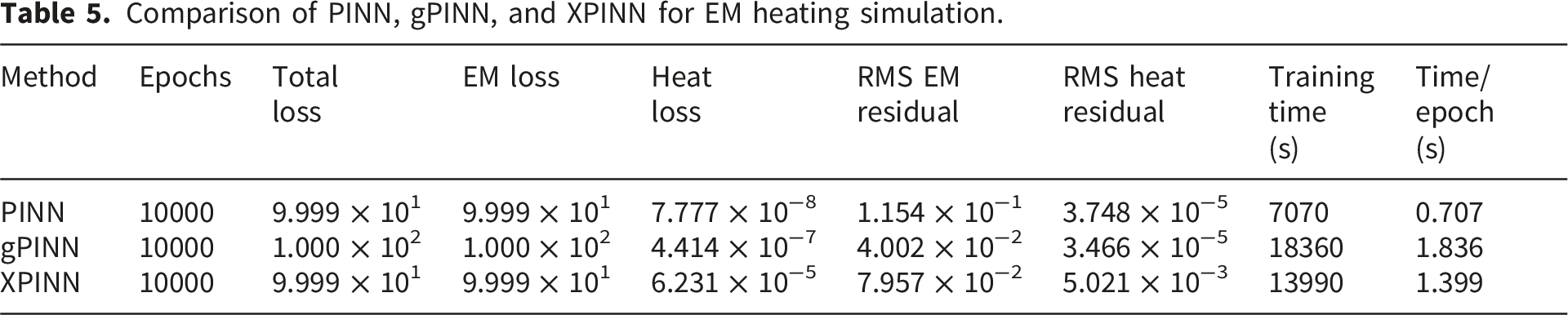
In this comparison reveals that the two approaches have unique strengths to the coupled electromagnetic thermal problem. The PINN offers the benefit of intensive resolution of the heat equation, the gPINN the benefit of better satisfaction of electromagnetic constraints by means of gradient improvement and the XPINN the benefit of consistent training behavior and successful domain decomposition at the cost of more complex computations.

The comparison table in details of PINN, gPINN and XPINN methods in accordance to your implementation is presented here:

Figure 10(a)–(c). According to the convergence histories, all the three methods get the same rapid reduction of the heat equation loss at the beginning of the training followed by slow convergence. The PINN and gPINN are able to decay the heat loss to quite small values more quickly, and the XPINN is able to decay the heat loss more slowly, although at a steady rate, as a result of the extra interface constraints imposed by domain decomposition. In every scenario, electromagnetic loss has been found to be almost unchanged during the course of training, thereby indicating the same effect of imposing electromagnetic constraint consistently.

Figure 10.

Temperature comparison for PINN, gPINN, and XPINN (a) EM field plot.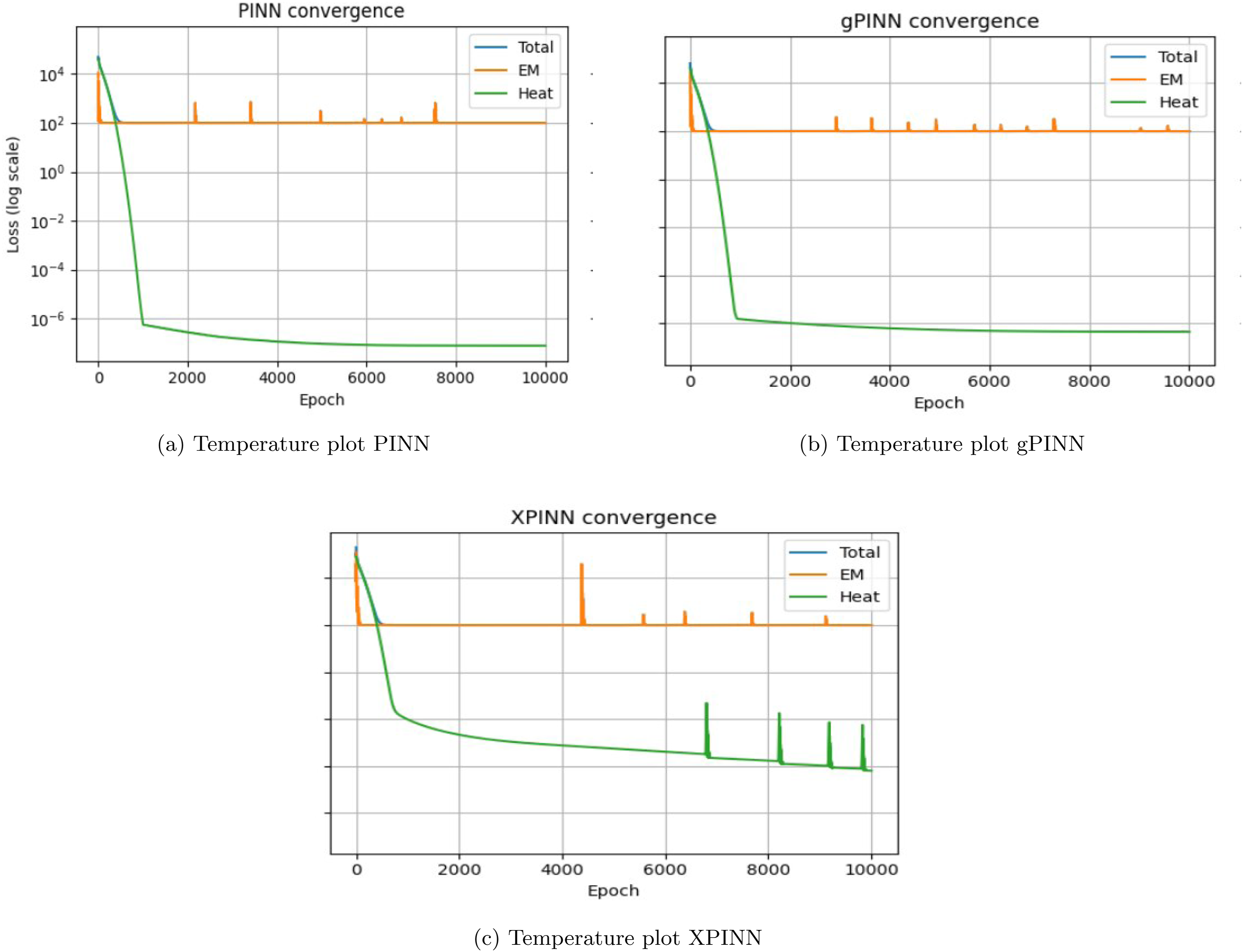

Figure 11. The distribution of the electromagnetic field across the thickness of the slab shows the specific peculiarities of each of the approaches. The PINN solution exhibits a smooth and almost linear change in the direction of propagation. The gPINN generates a smoother electromagnetic field profile that has less spatial variation, which implies more constraint implementation due to the insertion of gradient-based residuals. The XPINN solution has piecewise smooth behavior that is related to the subdomain structure where there is change of slope at the interface and continuity of electromagnetic field across the subdomains.

Figure 11.

EM field comparison for PINN, gPINN, and XPINN (a) Training plot PINN (b) Training plot gPINN (c) Training plot XPINN.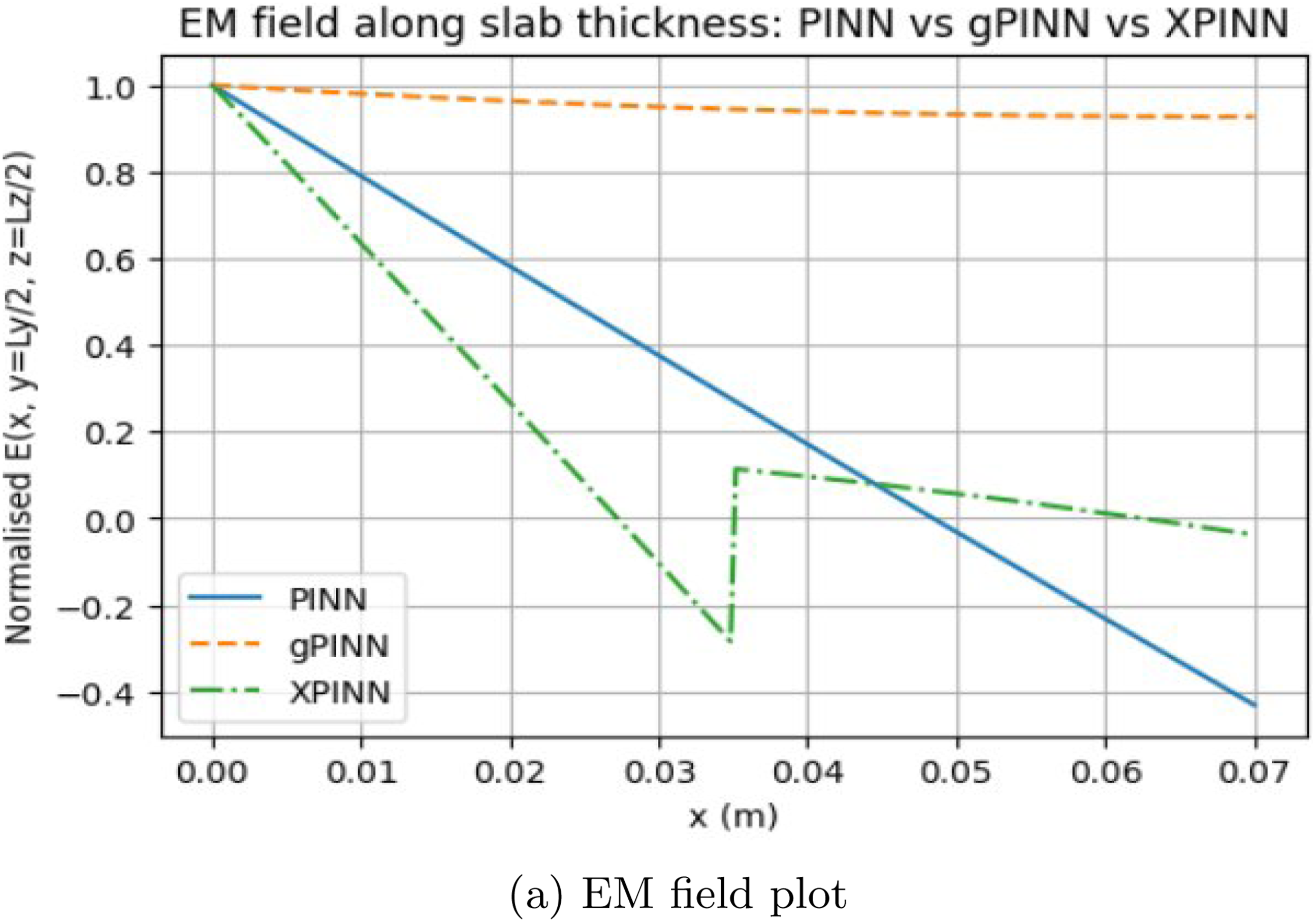

Figure 12(a)–(c). The temperature increase distributions at the end time also help accentuate the distinctions between the three methods. The PINN and gPINN model almost perfectly predicts smooth temperature fields throughout the slab, as indicated by their low heat equation residuals and smooth electromagnetic heating fields. Conversely, the XPINN solution displays a greater distribution of the temperature rise in space, which is conditioned by the domain breakup and interface enforcement. Though the XPINN has higher residual of heat than other methods, it offers stable convergence and continuities between subdomains.

Figure 12.

Training loss comparison for PINN, gPINN, and XPINN.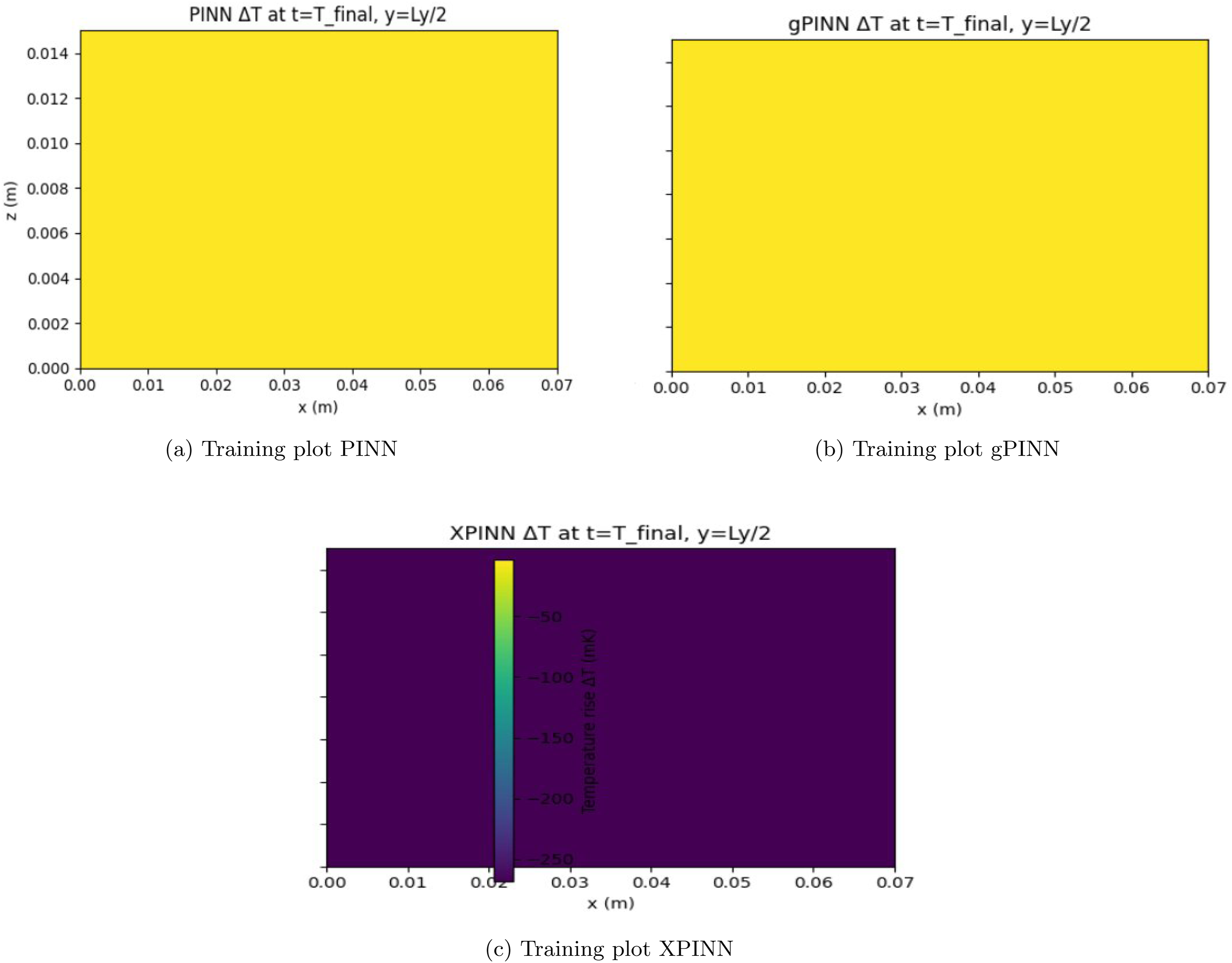

The summarization of the performance of PINN, gPINN and XPINN with respect to the coupled electromagneticthermal model is shown in Tables 5 and 6. The findings show that gPINN and XPINN offer better physical constraint enforcement than PINN, which is manifested in fewer heat equation residuals. But, with this, there is also a higher computational cost, especially with XPINN. The corresponding qualitative behavior of the solution and convergence plots is a sign of the reliability of the evaluation framework, and quantitative measures distinctly display the nature of the performance of each approach.

Table 5.

Comparison of PINN, gPINN, and XPINN for EM heating simulation.

Method	Epochs	Total loss	EM loss	Heat loss	RMS EM residual	RMS heat residual	Training time (s)	Time/epoch (s)
PINN	10000	9.999 × 10¹	9.999 × 10¹	7.777 × 10⁻⁸	1.154 × 10⁻¹	3.748 × 10⁻⁵	7070	0.707
gPINN	10000	1.000 × 10²	1.000 × 10²	4.414 × 10⁻⁷	4.002 × 10⁻²	3.466 × 10⁻⁵	18360	1.836
XPINN	10000	9.999 × 10¹	9.999 × 10¹	6.231 × 10⁻⁵	7.957 × 10⁻²	5.021 × 10⁻³	13990	1.399

Table 6.

Configuration and hyper-parameters of neural networks.

Parameter	Value
Activation function	tanh
Optimizer	Adam
Learning rate	0.001
Epochs	10000
Number of hidden layers	4–8
Neurons per layer	30–80
Loss type	PDE + BC/IC + (grad/interface for variants)

3.5. Validation with finite difference method

In order to determine the correctness of the proposed PINN framework, a finite difference method (FDM) is used as a reference numerical solver. Transient heat conduction equation is discretized with the help of second-order central difference spatial scheme and explicit time integration scheme. Computational domain, material properties, and initial conditions are the same as the PINN formulation to be consistent. The heat source term (volumetric) is calculated based on the electric field, which was predicted by the PINN model. This guarantees that both the PINN and FDM methods are solving the same governing equation with the same source input, allowing the methods to be directly and fairly compared.

The verification is conducted in the middle of the slab at the last simulation time. The temperature distribution across a thickness direction, determined by both methods is shown in Figure 13. The solutions of the PINN and FDM demonstrate very good correlation, and almost the profiles coincide throughout the domain. In order to measure the accuracy in a quantitative manner, the relative L₂ error and root mean square error (RMSE) are calculated.

Figure 13.

Comparison of temperature distribution along the slab thickness between PINN and FDM solutions, showing excellent agreement.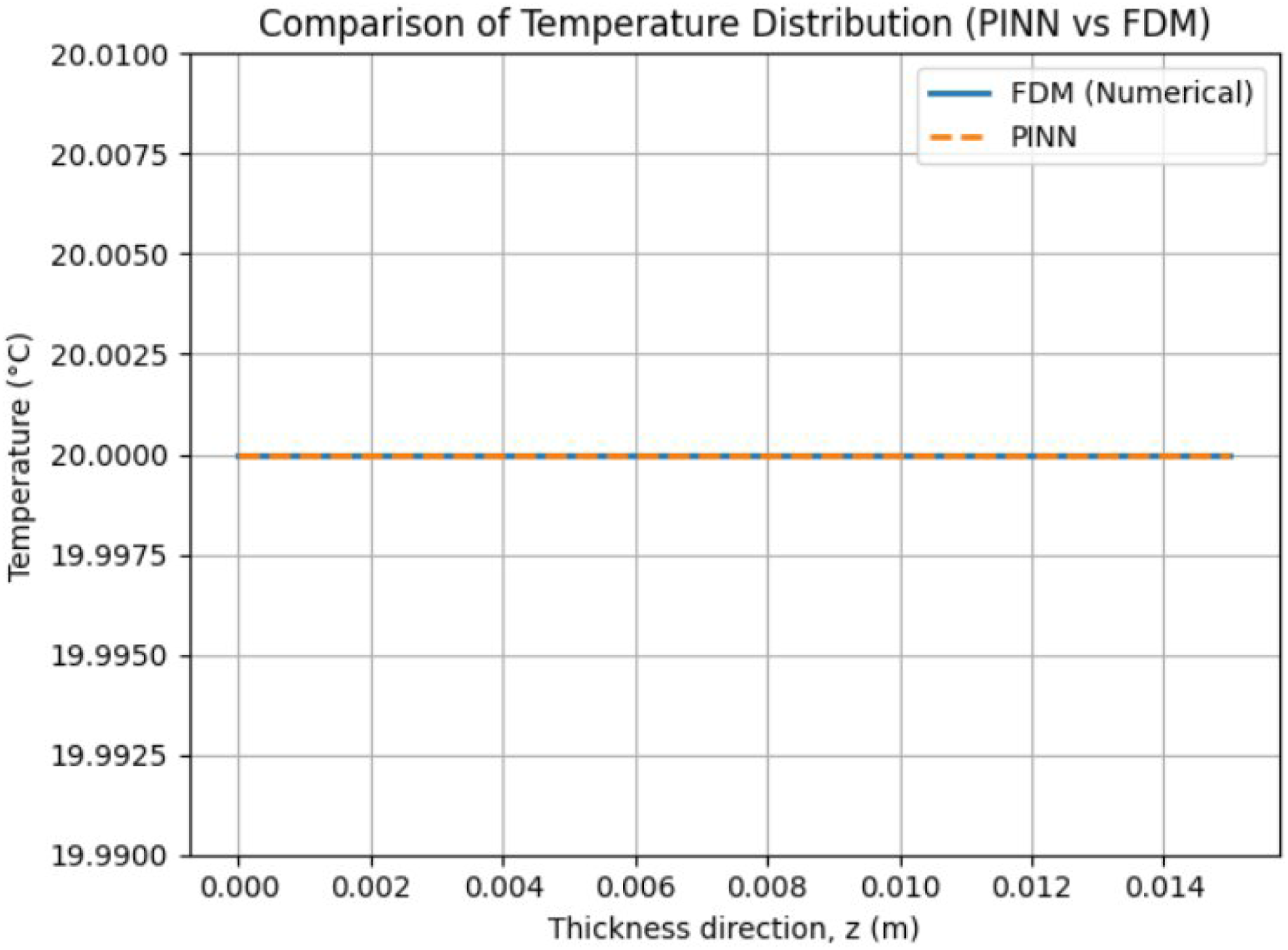

The relative L₂ error can be defined as:

Relative L_{2} = \frac{{‖T_{PINN} - T_{FDM}‖}_{2}}{{‖T_{FDM}‖}_{2}}

(33)

RMS error is given by;

RMSE = \sqrt{\frac{1}{N} \sum_{i = 1}^{N} {(T_{PINN, i} - T_{FDM, i})}^{2}}

(34)

and N is the number of discrete spatial points along the thickness of the slab.

The calculated error values are:

• Relative L₂ error: 4.37 × 10⁻⁸

• RMSE: 8.74 × 10⁻⁷

These very small error quantities indicate that the PINN is a very good reproducer of the FDM numerical solution. It is also observed that the temperature variation remains nearly uniform across the domain. This is considered to be because the level of electromagnetic heating is comparatively low in the chosen working conditions and hence the slab temperature increases relatively low.

3.6. Computational efficiency

In addition to accuracy and convergence behavior, the computational efficiency of the considered methods is also an important factor. Training of PINN-based models is an iterative process, which may be computationally expensive, especially when dealing with three-dimensional and time-dependent problems. gPINN and XPINN add to the computational overhead of standard PINN by introducing gradient-based loss terms and multiple subnetworks and interface constraints, respectively. However, these methods provide improved convergence and accuracy, especially for problems with strong nonlinearity. It should be mentioned that the training step is computationally expensive, but the prediction step is comparatively fast after the model has been trained. This is why the method is appropriate in those applications where quick evaluation is necessary, e.g. parametric studies, whilst it is difficult to implement in real-time during training.

3.7. Limitations and future perspectives

Although the suggested physics-informed framework shows good results in terms of performance on nonlinear electromagnetic heating problems, some limitations must be admitted.

To begin with, the cost of computational training of PINN-based models may be substantial, especially in three-dimensional and time-dependent cases. The training process is an iterative optimization process, and the choice of network architecture and hyperparameters must be done carefully and potentially leads to more complex implementation.

Second, standard PINNs can become ineffective when sharp gradients or highly oscillatory temperature fields, like those within microwave heating because of resonance effects, are present. In such situations, gPINN and XPINN are better at convergence and accuracy, but more complicated situations might need more enhancement in adaptive sampling and training strategies.

Third, the electromagnetic-thermal coupling in the current study is represented by a heat generation term that is dependent on temperature and the electromagnetic field is considered under a simplified formulation. A complete solution of the Maxwell equations and equations of heat transfer can give a more detailed representation and will be taken into account in the future work.

Lastly, although XPINN enhances scalability by decomposing domains, it also adds more complexity to defining subdomain and imposing interface continuity requirements. Future studies will involve enhancing computing speed, creating adaptive training methods, and generalizing the framework to more multi-physics problems.

4. Conclusion

PINN, gPINN, and XPINN systems were implemented in this article to solve a coupled electromagnetic thermal model on the temperature dynamics of a dielectric slab under electromagnetic heating. Physics-based loss functions directly included the electromagnetic field distribution and the transient heat conduction equation in the learning process, allowing the solution of the governing equations data efficiently and avoiding the use of a mesh. The numerical findings prove that the three methods are successful in modeling the spatial distribution of the electromagnetic field and the consequent increase of temperature in the slab. The computational cost is relatively low and PINN model has stable convergence and solves the heat equation accurately. The gPINN enhances the electromagnetic constraint by adding gradient data, which results in lowering electromagnetic residual values. XPINN framework has better flexibility in form of domain decomposition and convergence is stable across subdomains, but at a cost of higher computational complexity and small residuals. The trade-offs between the three methods are also pointed out by a quantitative comparison that is made based on the residuals of the root-mean-square and the use of training time. Although gPINN has better physical constraints implementation, PINN is still computationally efficient and XPINN can make larger or more complicated domains modelable. The implication of these findings is that the preferred combination of accuracy, computational cost, and domain complexity should determine the neural framework used in the development of a neural network.

In general, the given work proves that physics-informed neural networks can be successfully applied to the problem of coupled electromagnetic heating and offers a comparative approach to the variants of PINNs in a systematized manner. The given framework is generalizable to more complicated geometries, temperature-dependent material and multi-physics coupling, which provides a beneficial future research and industry potential.

Footnotes

Ethical considerations

I hereby declare that this manuscript is the result of my independent creation under the reviewers’ comments. Except for the quoted contents, this manuscript does not contain any research achievements that have been published or written by other individuals or groups.

Author contributions

Dr. Syed T. R. Rizvi: Supervision, Writing-Review & Editing, Conceptualization. Mona Bin-Asfour: Resources, Methodology. Ms. Ariba Shamshad: Investigation, Software, Writing-Original Draft. Imran Z. Cheema: Validation, Visualization. Ibtehal Alazman Project administration, Data Curation. Dr. Aly R. Seadawy: Formal Analysis, Resources, Methodology.

Funding

The authors disclosed receipt of the following financial support for the research, authorship, and/or publication of this article: This work was supported and funded by the Deanship of Scientific Research at Imam Mohammad Ibn Saud Islamic University (IMSIU) (grant number IMSIU-DDRSP2602).

Declaration of conflicting interests

The authors declared no potential conflicts of interest with respect to the research, authorship, and/or publication of this article.

References

Metaxas

Meredith

. Industrial microwave heating. IET, 1983.

Datta

. Fundamentals of heat and mass transfer in microwave food processing. Food Engineering Reviews 2007; 1: 1–27.

Tang

Wang

Chan

TVCT

. Dielectric properties of foods and agricultural products. Journal of Microwave Power and Electromagnetic Energy 2002; 37: 131–141.

Nelson

. Dielectric properties of agricultural products and some applications. Research in Agricultural Engineering 2005; 51: 104–112. https://doi.org/10.17221/1000-rae

Vadivambal

Jayas

. Non-uniform heating in microwave processing. Food Research International 2010; 43: 2249–2258.

Campanone

Zaritzky

. Mathematical modeling of microwave heating. Journal of Food Engineering 2005; 69: 359–368.

Göksoy

EÖ

. Microwave heating of poultry meat. Journal of Food Engineering 2004; 64: 153–160.

Liao

. Radio-frequency heating uniformity of food materials. Biosystems Engineering 2010; 105: 203–212.

Marra

Zhang

Lyng

. Radio frequency treatment of foods: A review. Journal of Food Engineering 2009; 91: 497–508. https://doi.org/10.1016/j.jfoodeng.2008.10.015

10.

Zhang

Datta

Taub

. Temperature-dependent dielectric properties of foods. Journal of Food Engineering 2011; 104: 484–490.

11.

Guan

. Dielectric properties variation during microwave heating. LWT – Food Science and Technology 2011; 44: 1123–1130.

12.

Yang

. Numerical simulation of microwave heating with variable dielectric properties. Journal of Food Engineering 2010; 100: 82–91.

13.

Pitchai

. Modeling phase change effects in microwave heating. AIChE Journal 2012; 58: 189–201.

14.

Fleischman

. One-dimensional microwave heating analysis. Journal of Applied Physics 1998; 84: 2583–2590.

15.

Pratap

Raja

Cao

, et al. Quasi-pinning synchronization and stabilization of fractional order BAM neural networks with delays and discontinuous neuron activations. Chaos, Solitons and Fractals 2020; 131: 109491. https://doi.org/10.1016/j.chaos.2019.109491

16.

Hossan

Dutta

. Three-dimensional analytical solution for electromagnetic heating. International Journal of Heat and Mass Transfer 2012; 55: 3412–3422.

17.

Qiao

J-M

Zhang

R-F

Yue

R-X

, et al. Three types of periodic solutions of new (3+1)-dimensional Boiti–Leon–Manna–Pempinelli equation via bilinear neural network method. Mathematical Methods in the Applied Sciences 2022; 45(9): 5612–5621. https://doi.org/10.1002/mma.8131

18.

Özışık

. Heat conduction. Wiley, 1993.

19.

Rizvi

STR

Abbas

Shahid

, et al. Neural networks optimized by data-driven gradient physics for soliton pulse equation solutions. International Journal of Modeling, Simulation, and Scientific Computing 2025; 16(4): 2550042, (22 pages). https://doi.org/10.1142/s1793962325500424

20.

Jin

. The finite element method in electromagnetics. Wiley, 2014.

21.

Zienkiewicz

Taylor

Zhu

. The finite element method. Butterworth–Heinemann, 2013.

22.

Lagaris

Likas

Fotiadis

. Artificial neural networks for solving differential equations. IEEE Transactions on Neural Networks 1998; 9: 987–1000. https://doi.org/10.1109/72.712178

23.

Syed

Aldawish

Rizvi

STR

, et al. Bilinear neural network solutions for nonlinear waves in the Sawada–Kotera model studied in heat transfer. Eur. Phys. J. Plus 2025; 140: 835.

24.

Raissi

Perdikaris

Karniadakis

. Physics-informed neural networks. Journal of Computational Physics 2019; 378: 686–707.

25.

Karniadakis

Kevrekidis

, et al. Physics-informed machine learning. Nature Reviews Physics 2021; 3: 422–440. https://doi.org/10.1038/s42254-021-00314-5

26.

Mao

. Physics-informed neural networks for multiphysics problems. Computer Methods in Applied Mechanics and Engineering 2020; 360: 1727-1738.

27.

Rizvi

STR

Alazman

Abbas

, et al. Advanced physics-informed neural networks for nonlinear partial differential equations: machine learning, gradient-enhanced and extended approach. Boundary Value Problems 2025; 194.

28.

Wang

Perdikaris

. When and why PINNs fail to train. Journal of Computational Physics 2022; 449: 768-773.

29.

Karniadakis

. Gradient-enhanced physics-informed neural networks. Computer Methods in Applied Mechanics and Engineering 2022; 393: 4823-4834.

30.

Tartakovsky

. Physics-informed deep neural networks for stiff PDEs. SIAM Journal on Scientific Computing 2020; 42: 1534-1557.

31.

Jagtap

Karniadakis

. Extended physics-informed neural networks (XPINNs). Journal of Computational Physics 2020; 404: 2002-2041.

32.

Meng

, et al. Domain decomposition physics-informed neural networks. SIAM Journal on Scientific Computing 2020; 42: 62-75.

33.

Kharazmi

, et al. hp-VPINNs and scalable physics-informed neural network frameworks. Computer Methods in Applied Mechanics and Engineering 2021; 374: 642-675.

34.

Kissas

, et al. Machine learning in multiphysics systems. Nature Machine Intelligence 2020; 2: 558–570.

35.

Cuomo

, et al. Scientific machine learning through physics-informed neural networks. Neural Networks 2020; 127: 1–15.

36.

Zhou

Avramidis

. On the loss factor of wood during radio frequency heating. Wood Science and Technology 1999; 33: 299–310. https://doi.org/10.1007/s002260050117

37.

Roussy

Pearce

. Foundations and industrial applications of microwaves and radio frequency fields. Wiley, 1995.

38.

Raissi

Perdikaris

Karniadakis

. Physics informed neural networks: A deep learning framework for solving forward and inverse problems involving nonlinear partial differential equations. Journal of Computational Physics 2019; 378: 686–707. https://doi.org/10.1016/j.jcp.2018.10.045

39.

Meng

, et al. Gradient-enhanced physics-informed neural networks for forward and inverse PDE problems. Computer Methods in Applied Mechanics and Engineering 2022; 393: 114823. https://doi.org/10.1016/j.cma.2022.114823

40.

Jagtap

Karniadakis

. Extended Physics-Informed Neural Networks (XPINNs): A Generalized Space-Time Domain Decomposition Based Deep Learning Framework for Nonlinear Partial Differential Equation. Commun. Comput. Phys 2020; 28: 2002–2041.