






Abstract
The current research evaluates the nonlinear motion of a spring pendulum system with a constant mass based on a variational approach. Using first principles, the Lagrangian of the model was created in polar coordinates, which produced the Euler-Lagrange equations that describe the motion of the radial and angular components as functions of each other. Under the premise of small oscillation, the equations were simplified into a more easily solved nonlinear equation. To provide accurate analytical solutions for large timescales, the Ms-VIM) solution technique was used to overcome the limitations associated with the convergence rate of the classical VIM solution technique. In addition to the analytical solutions obtained, the solutions were also evaluated using the fourth order Runge-Kutta (RK4) method. An assessment of the analytical and numerical solutions indicated very good agreement among them, indicating that the proposed solution technique was reliable and efficient. Phase plots and error analyses were also conducted to illustrate the nature of the motion and the stability characteristics of the system. This research provided a viable analytical-numeric solution strategy for evaluating the motion of a constant mass oscillating system and can be applied to more complicated nonlinear mechanical models.
1. Introduction
Spring-pendulums are an example of a nonlinear oscillator; they can produce a vast array of nonlinear behavior, including amplitude dependent frequencies, bifurcation, and nonlinear energy transfer between interacting modes.1–3
A typical example of a strongly nonlinear mechanical system that displays all of these nonlinear behaviors is the classical spring pendulum4–6; this model exhibits both radial and angular motions. Due to the strong coupling between the extension of the spring and the rotation of the pendulum, the length of the pendulum changes during motion producing complex behavior including nonlinear resonances, internal energy transfer, and modulation of oscillation amplitudes.7–9
Therefore, the spring pendulum model is a classic representation of a nonlinearly coupled mechanical system; it is a representative system for illustrating the effects of nonlinear coupling on the dynamics of a mechanical system. 10
Additionally, the motion of the spring pendulum has application to many engineering disciplines, including crane payload dynamics, robotic manipulator design with flexible links, vibration control devices, and aerospace tether systems.11,12 A better understanding of the nonlinear interactions between the radial and angular motions will help engineers to design mechanical systems that are stable and perform well under dynamic loading.
The motion of the spring pendulum can be described using Lagrange’s equations of motion. The Lagrange equations of motion are a general method for determining the equations of motion of a nonlinear dynamical system with many degrees of freedom.13–15 The Lagrange method uses the total energy of the system, which includes both the kinetic and potential energies, to derive the equations of motion of the system. The Lagrange method is commonly used in classical mechanics and nonlinear dynamics for determining the equations of motion of systems that can be described using generalized coordinates.16–18 Additionally, the Lagrange method can be used to extend the description of a system to include dissipative forces through the use of the Rayleigh dissipation function.19,20
Due to the highly nonlinear form of the equations of motion of the spring pendulum, exact analytical solutions cannot be found using the Lagrange method or other analytical methods. Therefore, a number of analytical and numerical approximation methods have been developed to study the nonlinear vibrations of the spring pendulum. Classical perturbation methods such as the method of multiple scales, the harmonic balance method, and the averaging method have been widely used to study nonlinear oscillation problems.21–23 However, these classical perturbation methods typically rely on a small parameter and can lose their accuracy if the nonlinearity becomes large or if long time simulations are necessary. Recently, other efficient analytical techniques have been developed for nonlinear oscillators, including He’s frequency method and the spreading harmonic balance method (see recent works in Fractals and related journals). These methods are highly effective for frequency-amplitude analysis, but the present study focuses on long-time integration of coupled state variables using the multi-stage variational iteration method.
In response to the limitations of classical perturbation methods, a number of new semi-analytical methods were developed in the late twentieth century. One of the most successful of these semi-analytical methods is the Variational Iteration Method (VIM), which was developed by He.24,25 The VIM uses the principle of variation to construct a correction functional that converges rapidly to the exact solution of the equation. This correction functional is constructed using a Lagrange multiplier, and the resulting iterative formula does not involve linearization or discretization. The VIM has been shown to be useful for solving a wide range of nonlinear problems in physics and engineering.26,27
Recent extensions of the VIM include the dual Lagrange multiplier approach, 28 which introduced two Lagrange multipliers to solve two-point boundary value problems in nonlinear oscillators. This innovation expands the VIM to a new class of problems beyond traditional initial value problems. While their method focuses on conservative single-DOF systems with boundary conditions, our work addresses the complementary challenge of long-time integration of initial value problems in coupled, multi-DOF systems with damping, using the multi-stage VIM formulation.
Although the VIM has several advantages, one of its main disadvantages is that it produces a local series solution, and the size of the convergence region for this solution can limit the accuracy of the solution over long periods of time. For example, in the case of nonlinear dynamical systems, the accumulation of truncation errors over time can lead to significant differences between the approximate solution and the actual solution. To improve the accuracy and robustness of the VIM for simulating long time responses, the Multi-Stage Variational Iteration Method (Ms-VIM) was developed as an improved version of the VIM. 25 The Ms-VIM divides the time interval into smaller sub-intervals and reconstructs the solution at each stage using the updated initial condition. This multi-stage approach substantially improves the accuracy and reliability of the Ms-VIM for simulating long time responses of nonlinear dynamical systems.
In recent years, researchers have focused an increasing amount of research on nonlinear dynamics in elastically-coupled systems such as the spring-pendulum and oscillation systems with relevance to applications in engineering. Amer et al.,29,30 used numerical analysis to model the motion of a spring pendulum under planar forced motion and found that both nonlinear coupling and forcing significantly affect the system’s dynamics. The authors also applied the same approach to analyze a two degree of freedom spring pendulum traveling along a Lissajous path and illustrated how strong modal interaction can produce complicated oscillations. Additionally, Rouleau et al. 31 investigated the nonlinear transition and periodic response of elastically-coupled pendulums and Szumiński and Maciejewski 32 investigated the dynamics and nonintegrability of the double spring pendulum to demonstrate the potential complexity and sensitivity of strongly coupled nonlinear oscillators. All these investigations highlight the need for well established analytical-numerical methods that will allow the investigation of nonlinear spring pendulum systems over large periods of time.
Moreover, studies in recent years have explored fractal and fractional formulations of nonlinear pendulum oscillators in an attempt to better reproduce complex dynamic behaviors. In 33, the authors investigated the numerical response of a fractional rotating pendulum system and showed the influence of fractional parameters on oscillatory behavior and stability. In a similar direction, 34 studied the nonlinear dynamics of a rolling wheel pendulum using numerical methods. The sensitivity of the system to fractal effects and parameter changes is emphasized. In addition, 35 offered analytical solution procedures for the same class of oscillators, giving approximate formulations to supplement numerical results. These works collectively highlight the increasing significance of fractal and fractional modelling in the context of nonlinear vibration analysis and propel the design of robust iterative schemes for solving intricate oscillatory systems.
This paper presents an investigation of the nonlinear dynamics of a spring pendulum system using the Multi-Stage Variational Iteration Method. Both conservative and damp cases are examined. The Ms-VIM is used to find the semi-analytical solutions of the system, and the numerical reference solutions are generated by the classical fourth-order Runge-Kutta method. By comparing the analytical and numerical solutions, the accuracy, stability, and convergence properties of the proposed Ms-VIM method can be evaluated. The comparisons show that the multi-stage formulation of the VIM improves its ability to predict the behavior of the system and provide reliable solutions for the nonlinear oscillatory systems. Therefore, the proposed framework is a powerful and efficient analytical-numerical tool for studying nonlinear mechanical systems and can be expanded to more complex dynamical systems encountered in modern engineering applications.
2. Physics of the model
Below is an illustration of a spring pendulum with a mass
First, we must determine the mass’s


In terms of polar coordinates


Finally, the Lagrangian (

Below, we will use (10) and the relation
In this case, θ is very small and thus


This second-order approximation retains the essential nonlinear coupling term
Applying (6) directly to (5). Thus

Simplyfing


Simplifying

While for

Simplifying

Now, let us assume that the spring pendulum is subject to a viscous daming that opposes both the radial and angular motions. The dissipative effects can be introduced through the Rayleigh dissipation function defined as



3. Method of solution
In this section, we present the fundamental concepts of VIM. The findings presented here are also available in 21 and the works referenced therein.
3.1. He’s variational iteration method
Consider, at this point, the following system:


The VIM can be regarded as a modification of the Lagrange multiplier method. 22 In what follows, we briefly review the Lagrange multiplier method and clarify its connection to VIM. This presentation is adapted from. 36
An initial function

This yields an approximation at
According to J. H. He,
37
the correction functional is given by:

The function
The method is essentially based on defining a Lagrange multiplier that meets the following condition (see 40)

Classical VIM provides a local series solution expanded about the initial time, whose validity is limited by a finite radius of convergence. In nonlinear systems, this local nature leads to rapid accumulation of truncation and phase errors when the method is applied over long time intervals. Increasing the number of perturbation terms improves local accuracy but does not guarantee global reliability. Ms-VIM overcomes this limitation by subdividing the time domain and reconstructing the VIM soluıtion at each subinterval using updated initial conditions. This reinitialization maintains the solution within the convergence region of the local series, thereby enhancing long-time accuracy and stability. Consequently, Ms-VIM is more suitable than classical VIM for long-time integration of nonlinear dynamical systems.
3.2. Multi-stage variational iteration method
Batiha et al. developed the Ms-VIM
41
to improve the performance of VIM on extended time intervals. The Ms-VIM approach determines the solution of equation (16) on

A practical note on subinterval size selection: smaller subintervals improve accuracy but increase computational cost. Users should adjust the subinterval size according to the nonlinearity and stiffness of the system. In this study, the same step size is used for both the Ms-VIM and the RK4 method.
Case 1
The subsequent analysis applies methods VIM and Ms-VIM to equations (14)-(15). To rewrite Eqs. (9)–(10) as a first-order system, we introduce the state variables

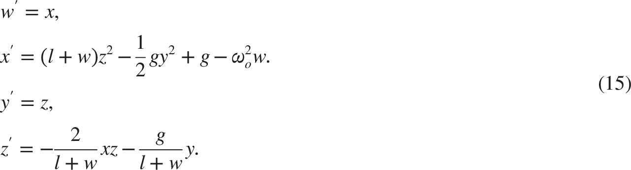
Using these definitions, Eqs. (9)–(10) can be equivalently written as the following system of four first-order differential equations
The corresponding initial conditions become

This representation expresses the second-order system (9)–(10) as an equivalent four-dimensional first-order dynamical system, which is suitable for analytical techniques (Variational iteration method and multi-stage Variational iteration method) as well as for numerical solvers such as the fourth order Runge–Kutta method.
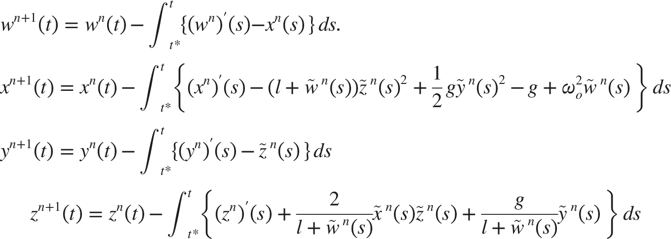
Based on the classical VIM approach widely adopted in the literature, the following correction functionals are derived:
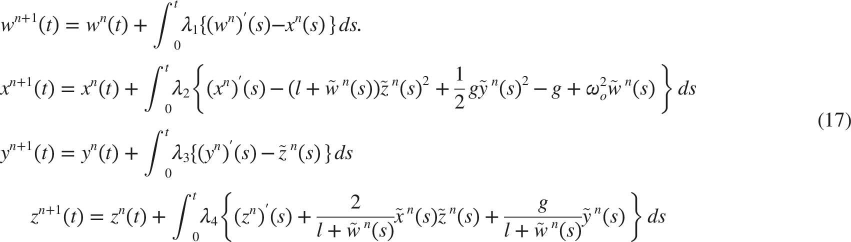
Notably, several linear terms in (17) are imposed as restricted variations, simplifying the process of identifying the Lagrange multipliers. The Lagrange multipliers are obtained by computing the variation of the correction functionals, namely:
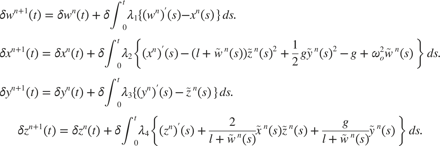
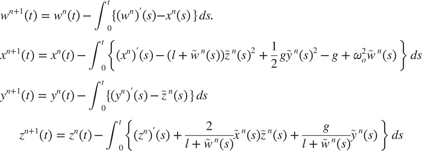
Through integration by parts and the calculus of variations, we obtain the Lagrange multipliers in the form:

As a result, the correction functionals corresponding to VIM can be written as:
Case 2
In order to transform Eqs. (12)–(13) into an equivalent first-order system, we define the state variables as follows:

Employing these definitions, Eqs. (12)–(13) take the form of the following system consisting of four first-order differential equations:
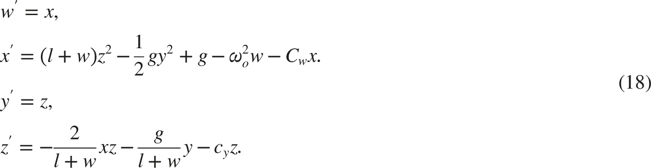
Under this formulation, the initial conditions become:

This formulation converts the second-order system (12)–(13) into an equivalent four-dimensional first-order dynamical system, making it appropriate for analytical approaches such as the VIM and the Ms-VIM, as well as for numerical schemes like the classical fourth-order Runge–Kutta method.
By applying the classical VIM scheme frequently used in earlier works, we formulate the correction functionals as:
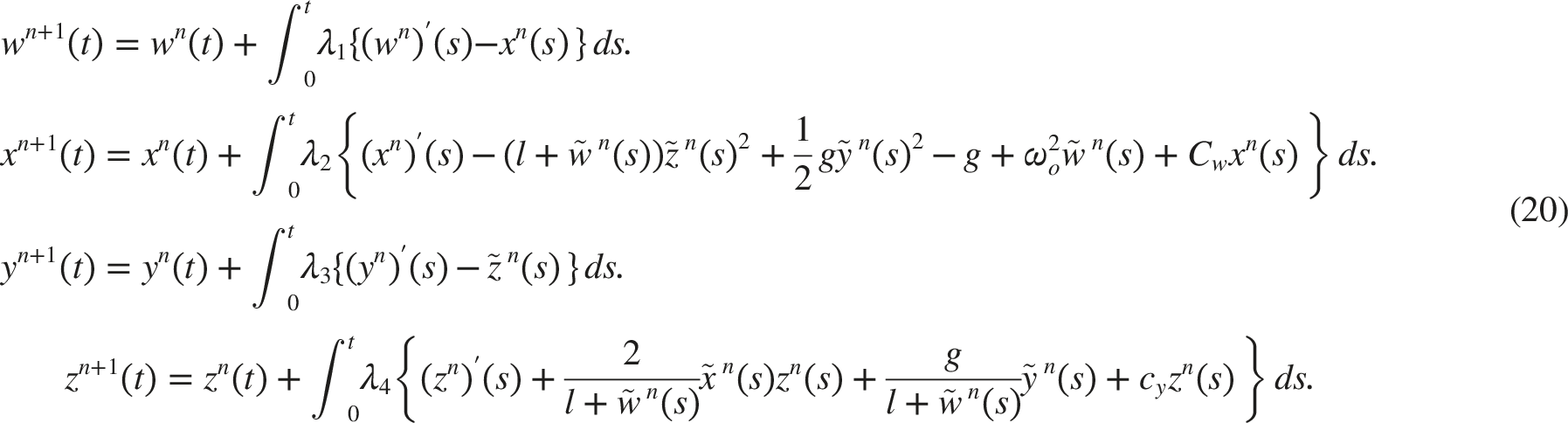
It is worth noting that several linear terms in (20) are treated as restricted variations, which facilitates the identification of the Lagrange multipliers. These multipliers are determined by taking the variation of the correction functionals, namely:
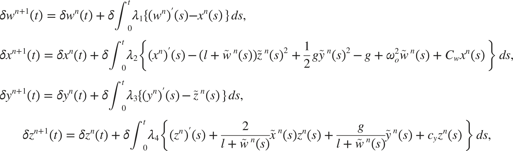
The Lagrange multipliers are subsequently derived, via integration by parts and variational analysis, as follows:

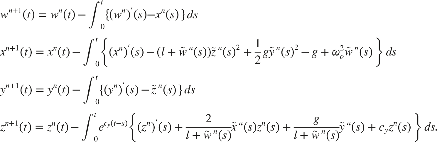
By taking
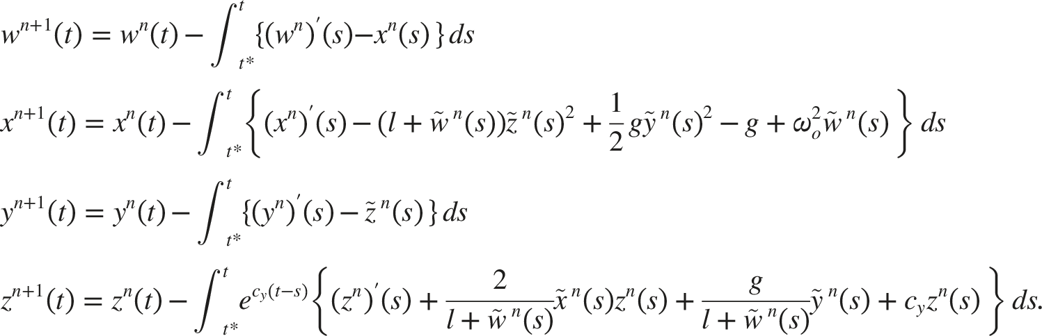
4. Results
The multi-stage variational iteration method algorithm is implemented using the computer algebra system Matlab. A fixed step size of
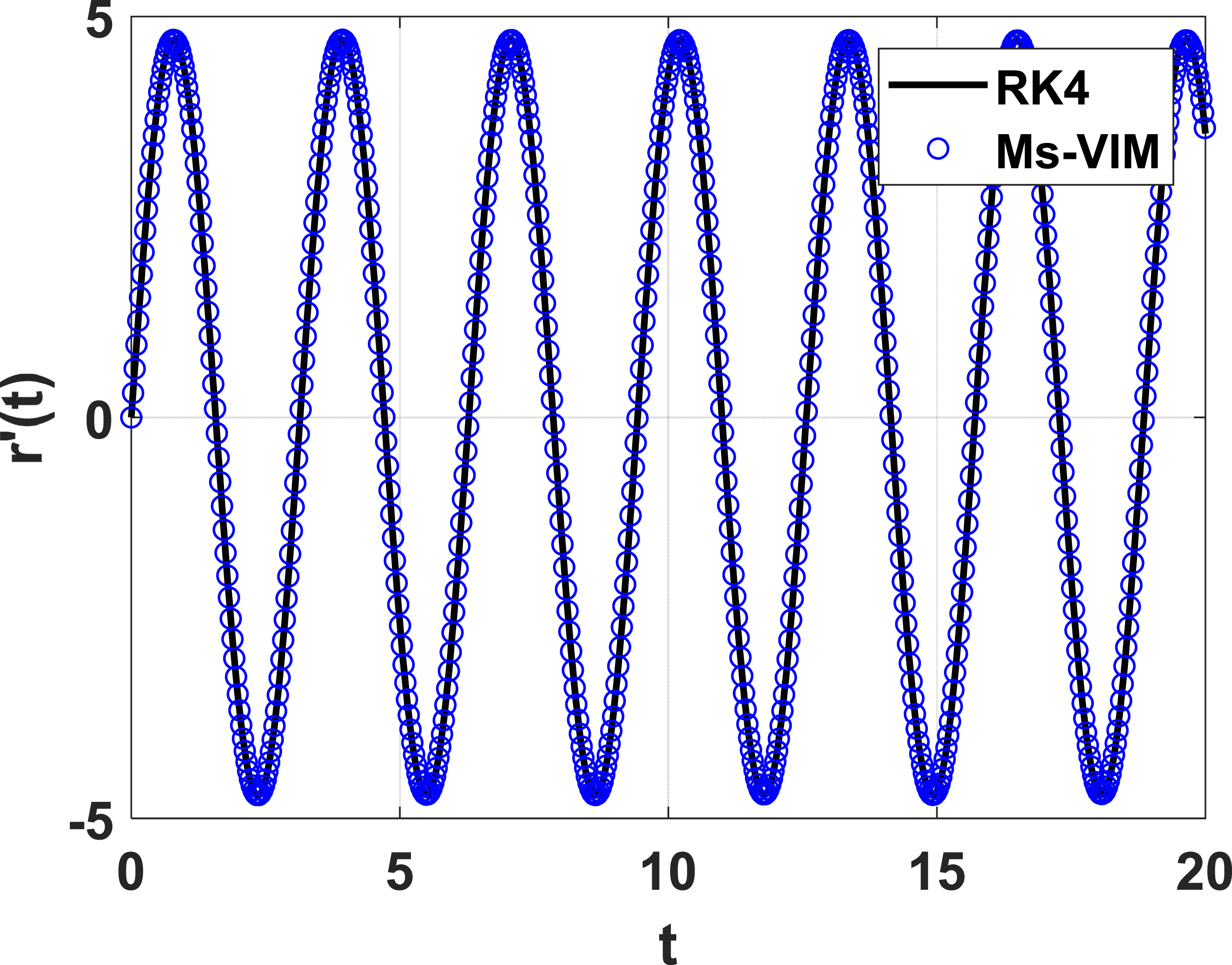
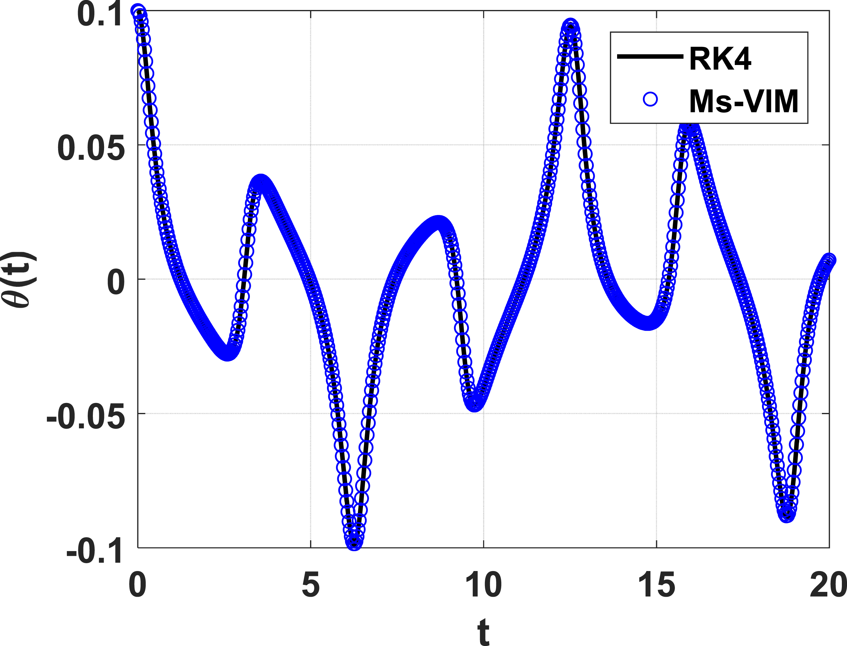
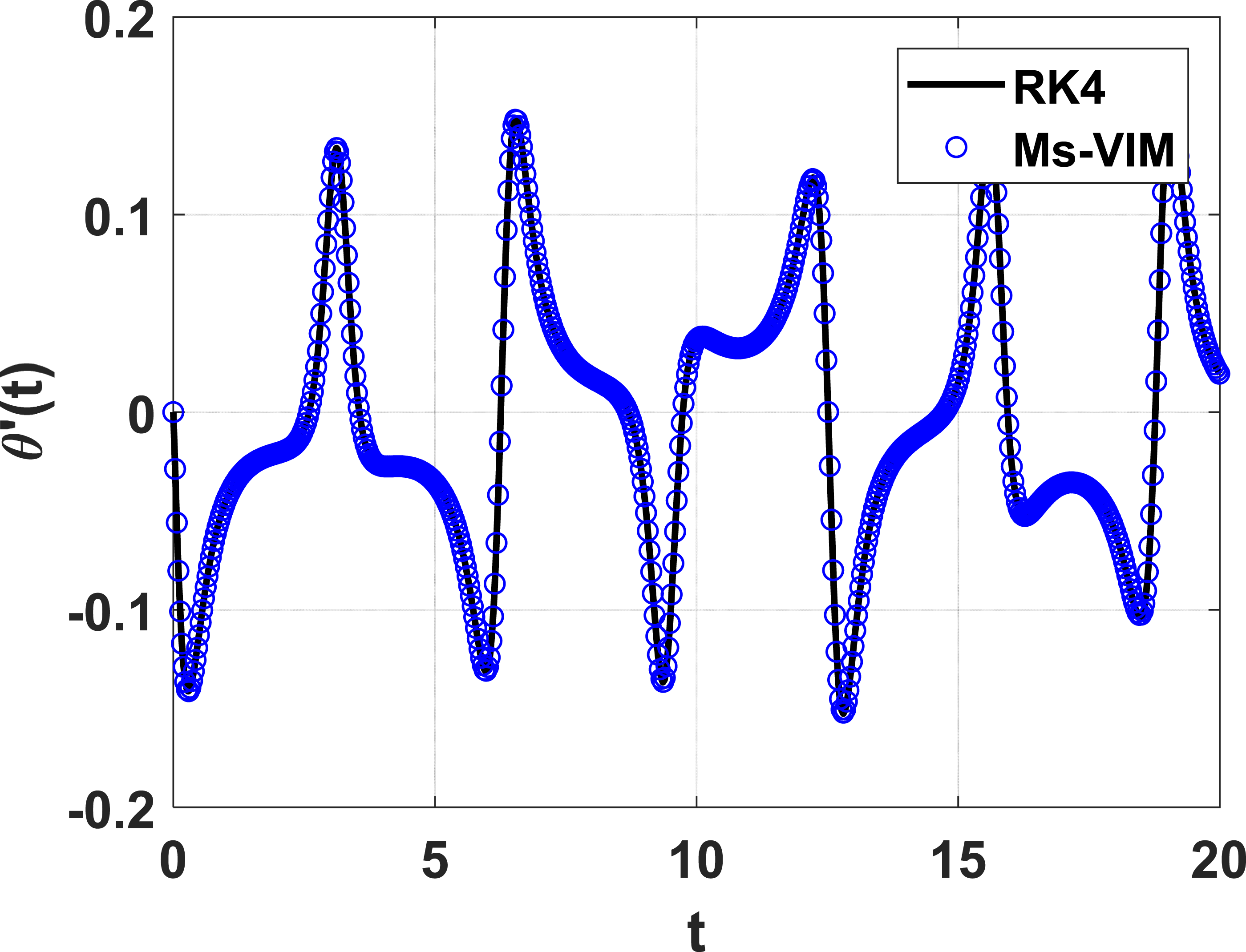
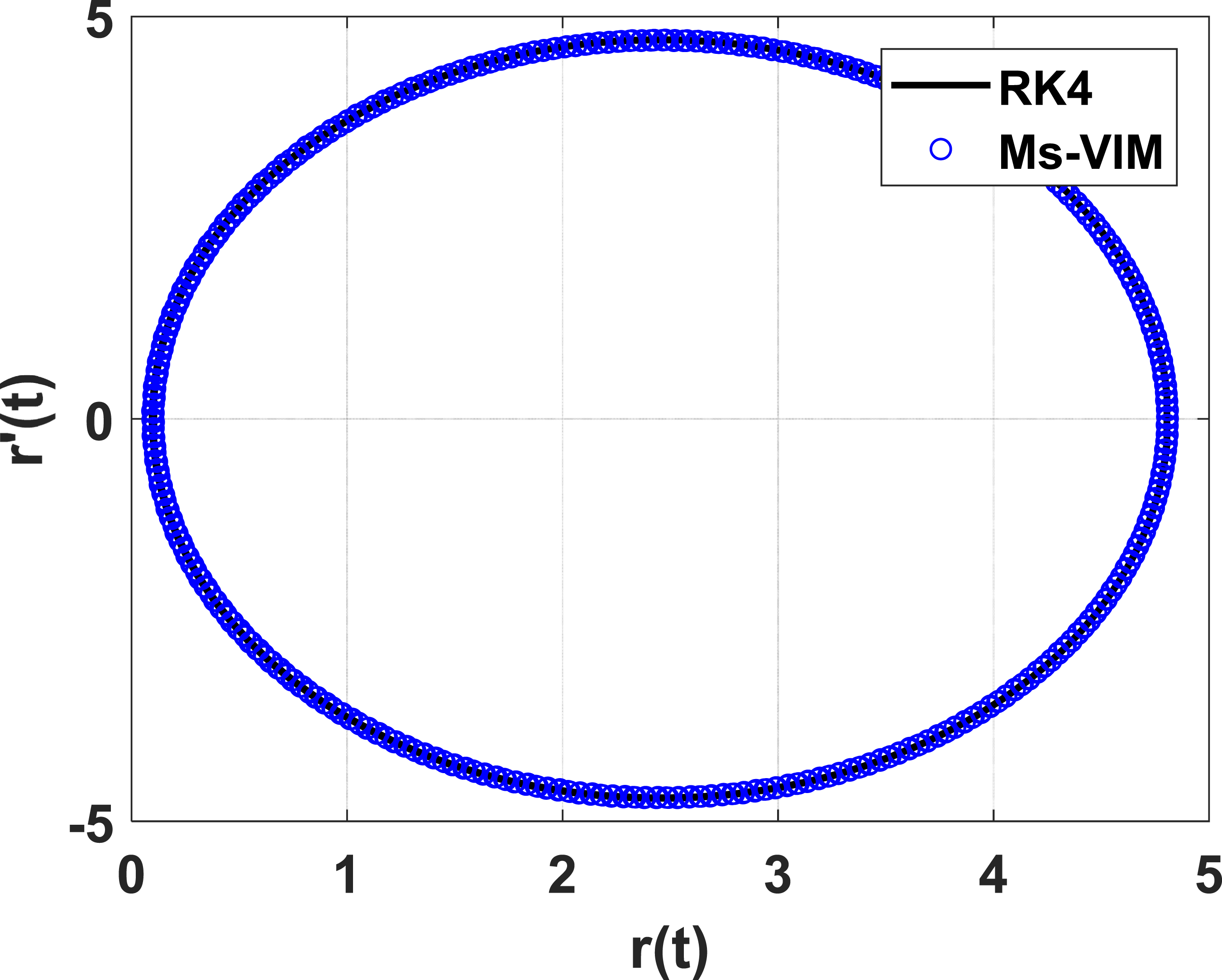
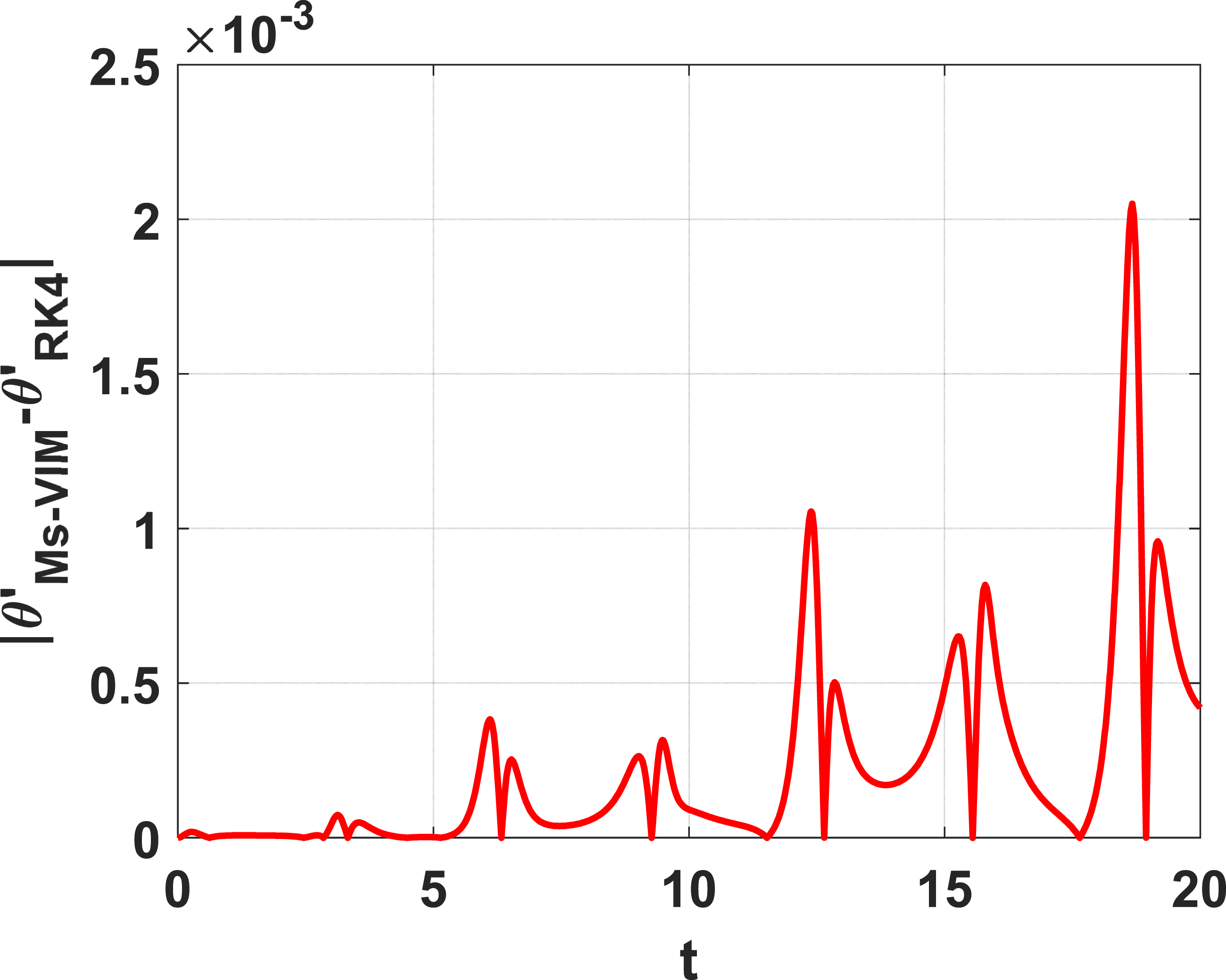
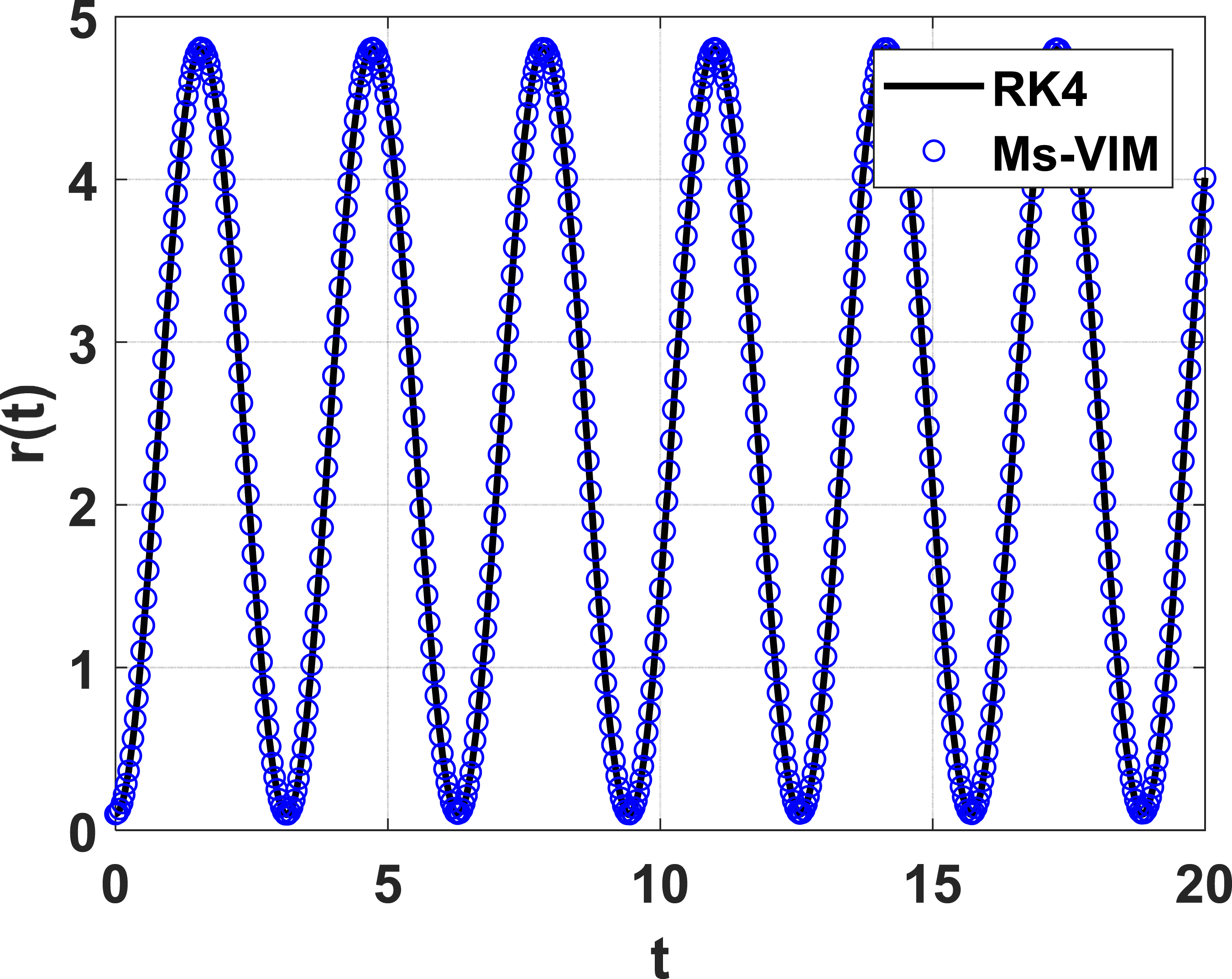
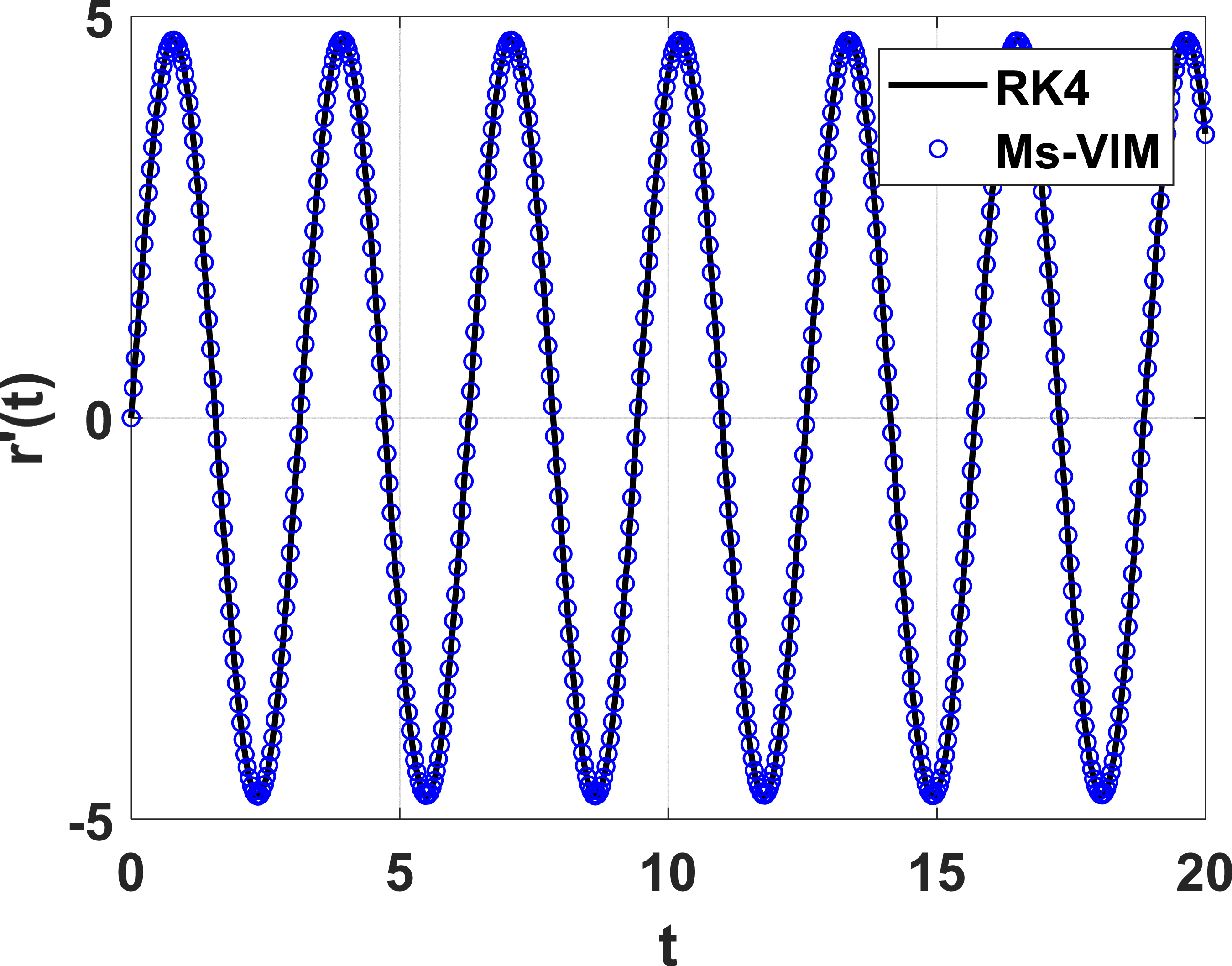
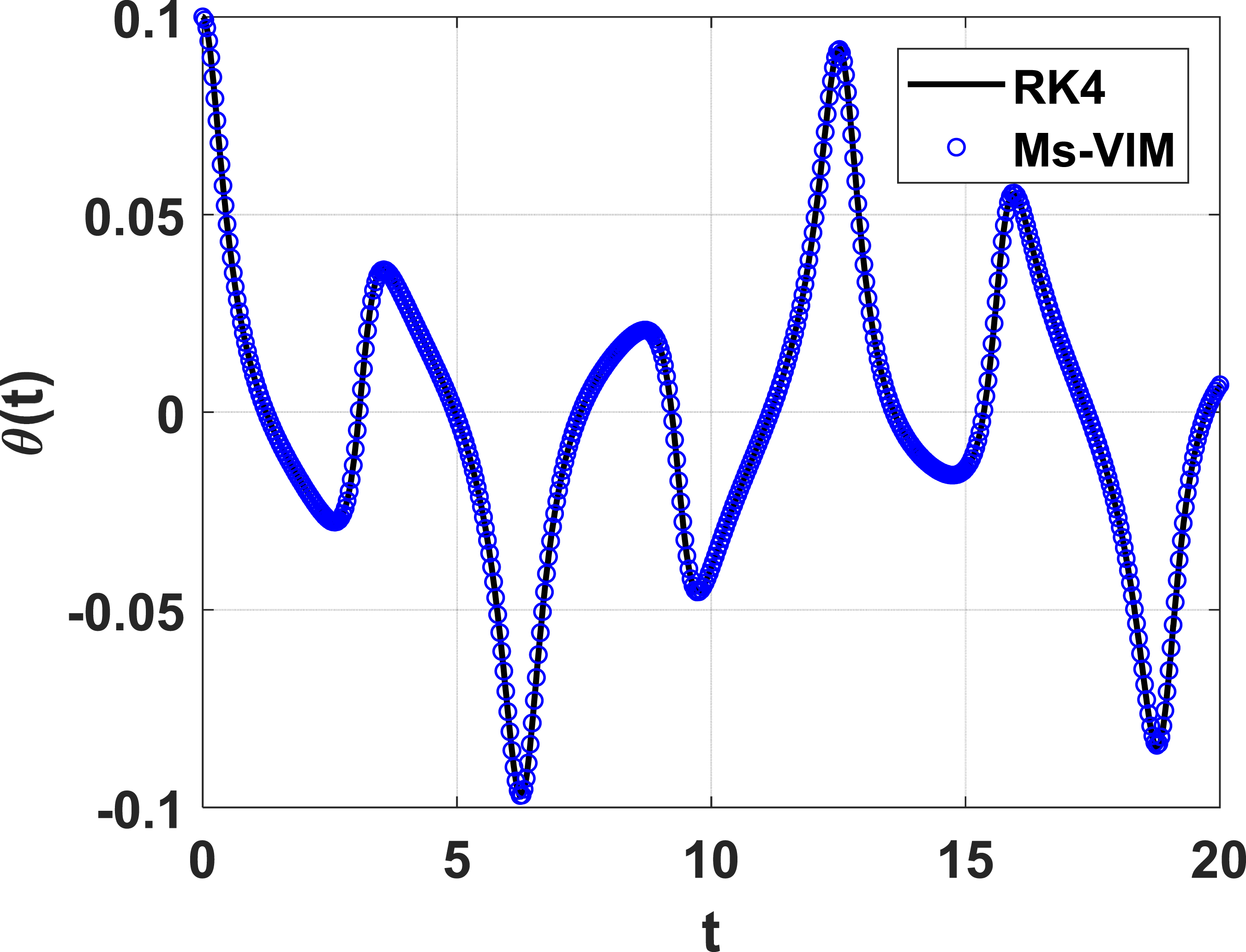
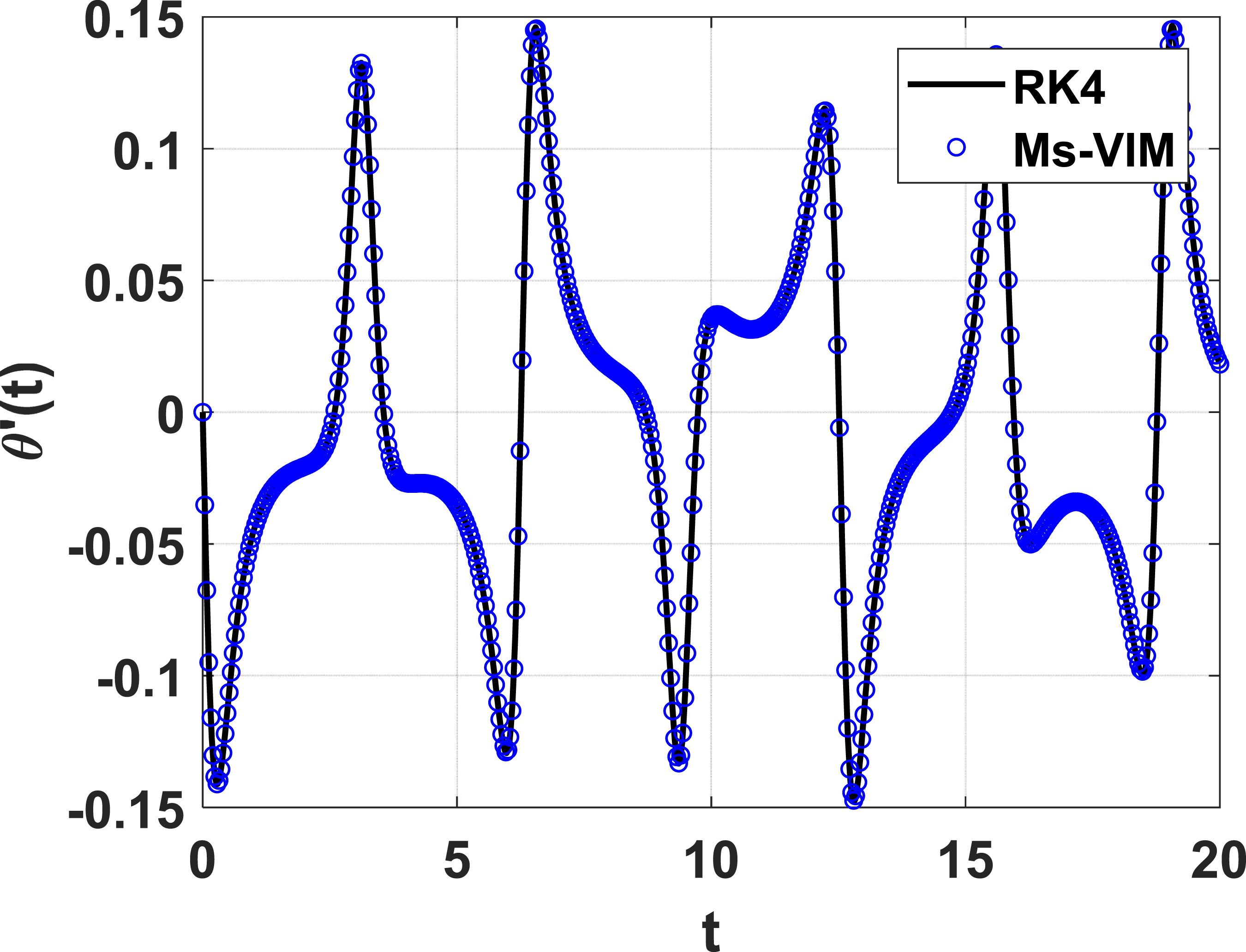
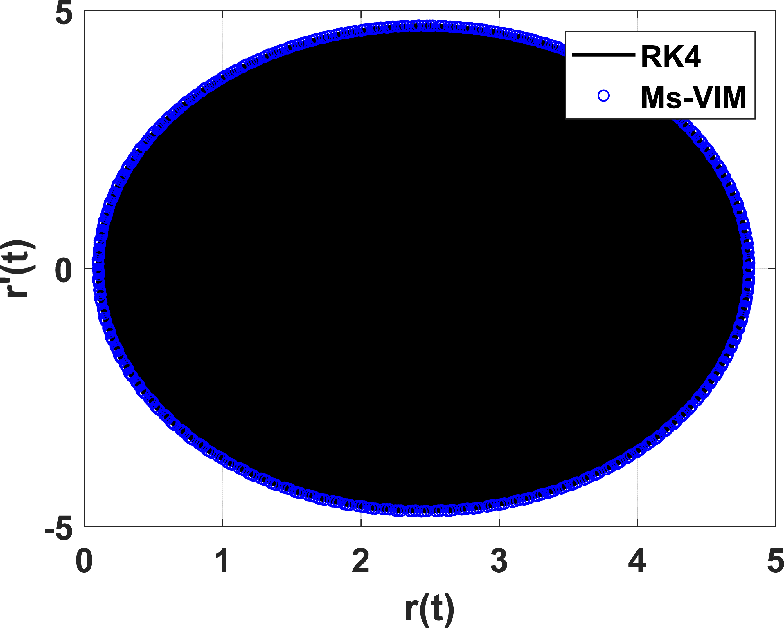
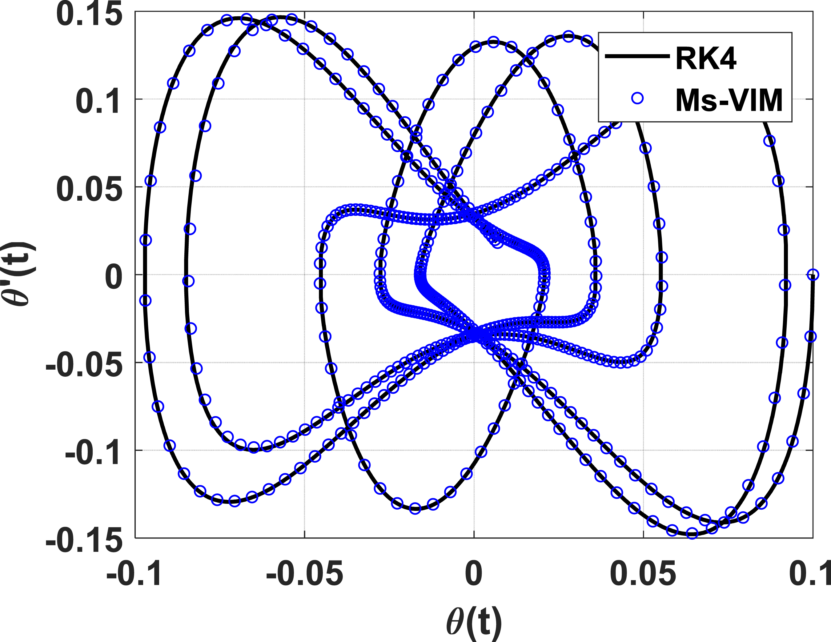
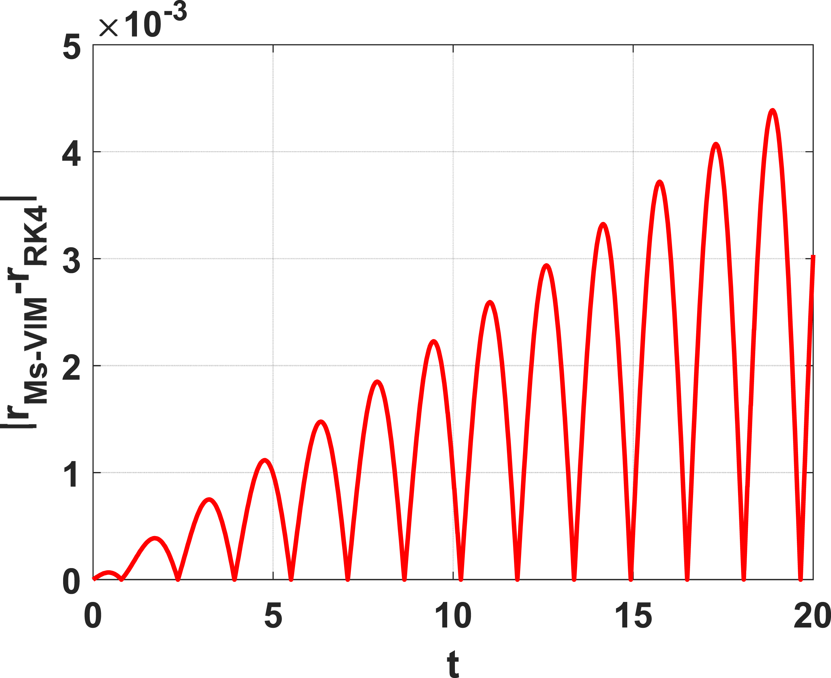
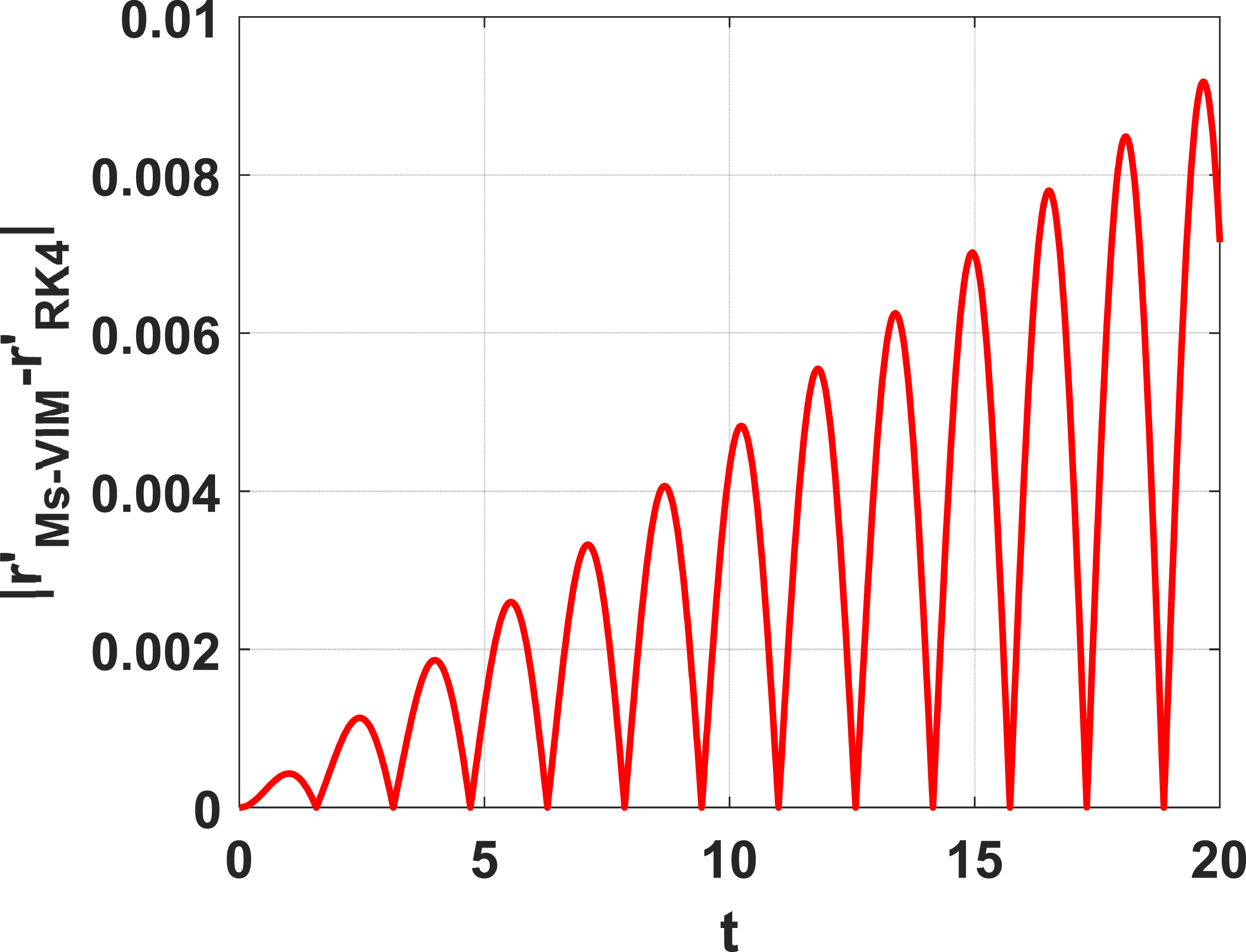
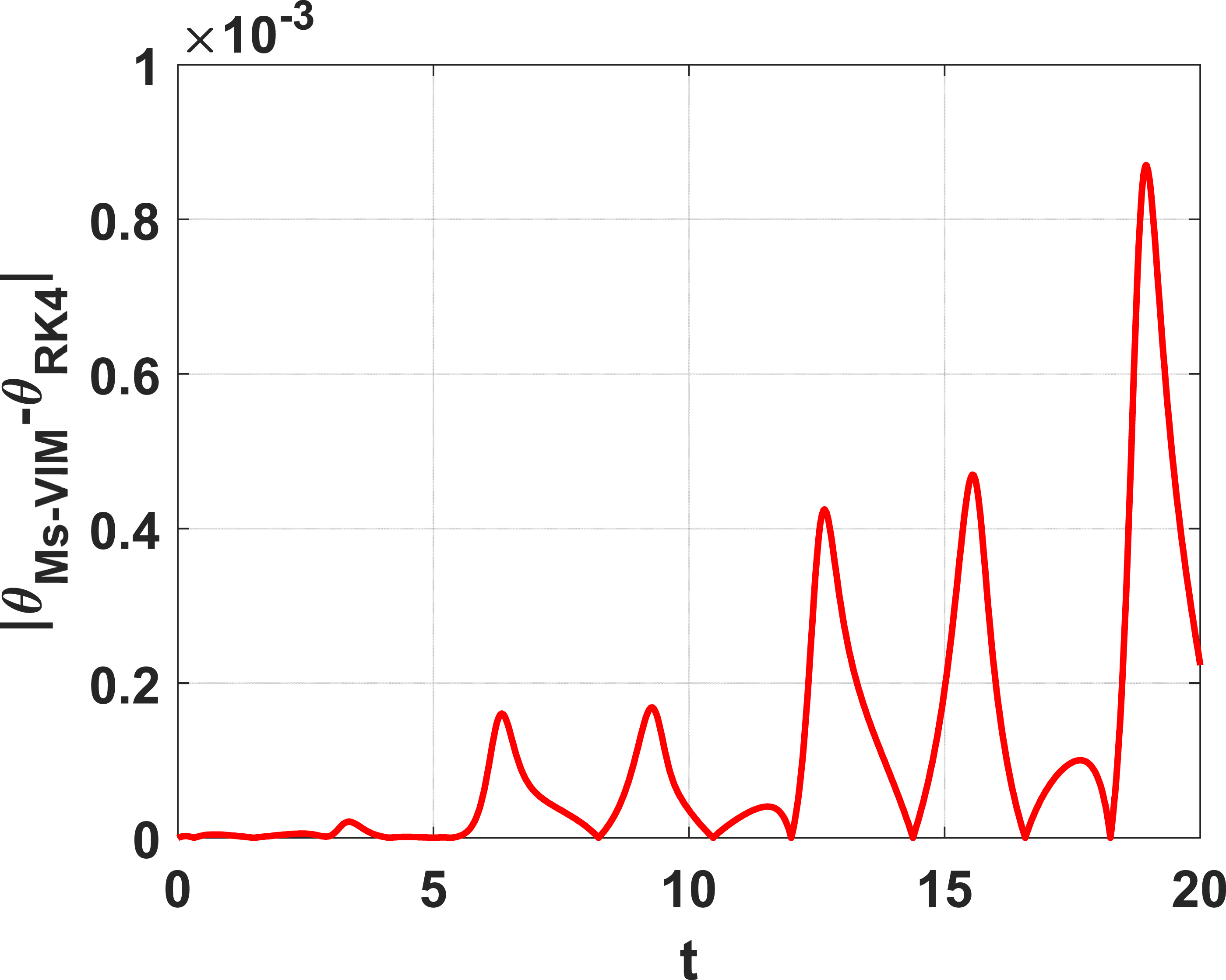
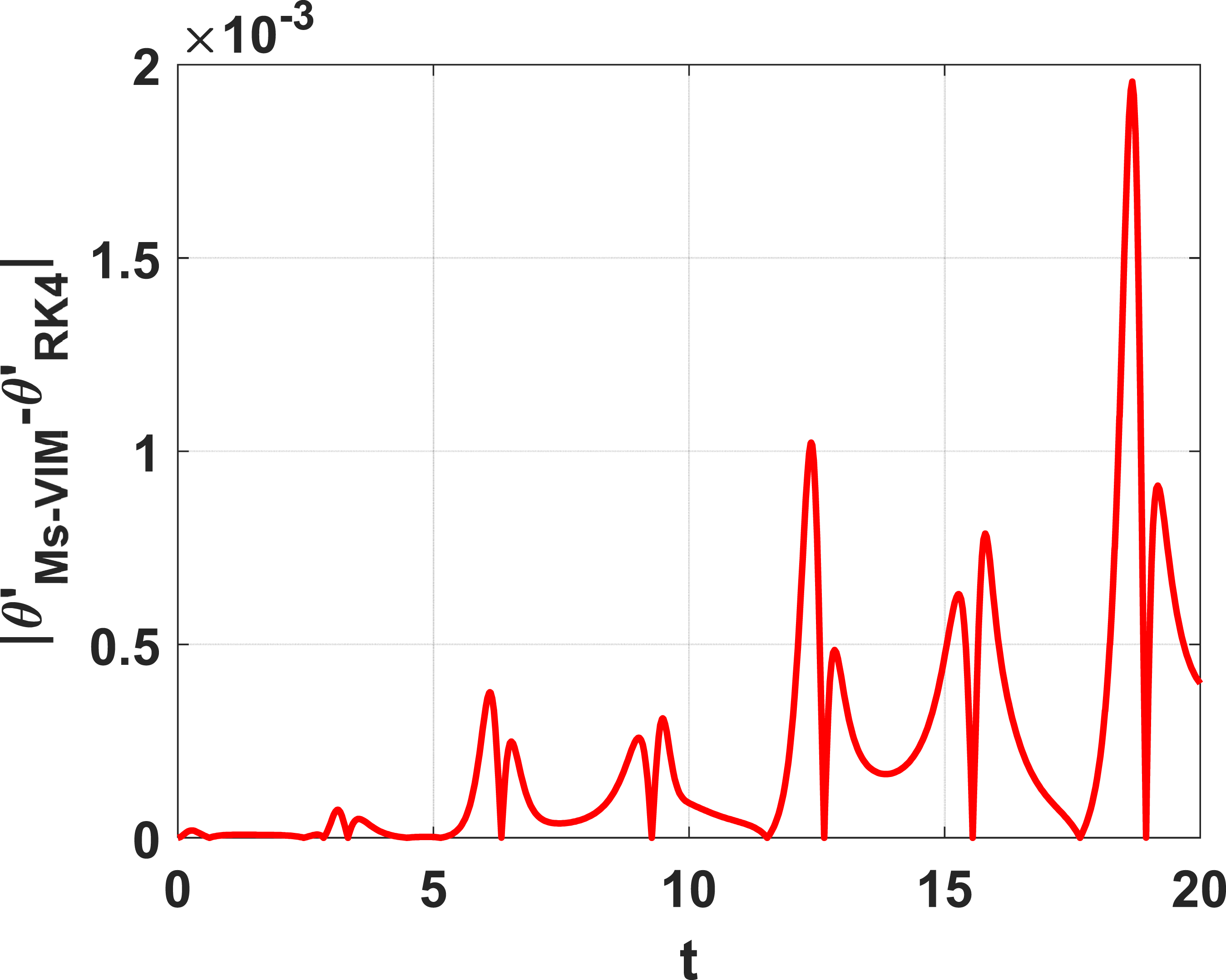
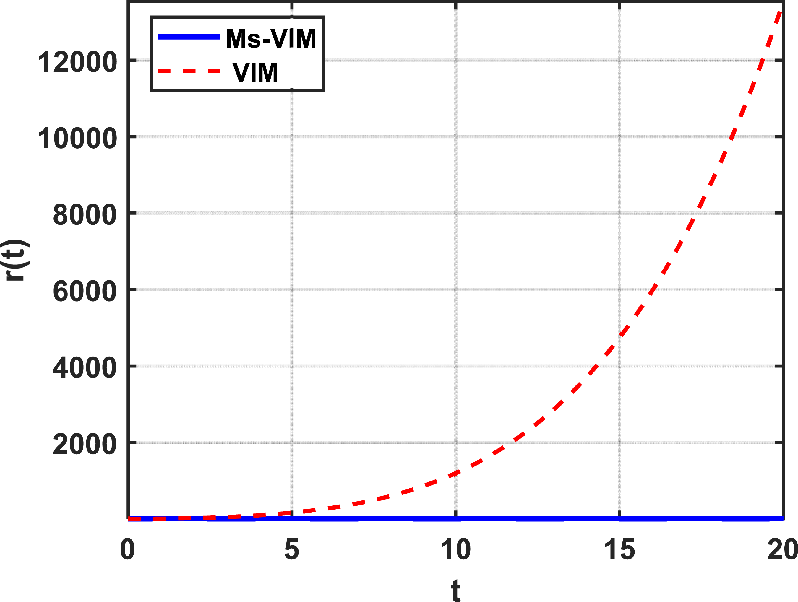
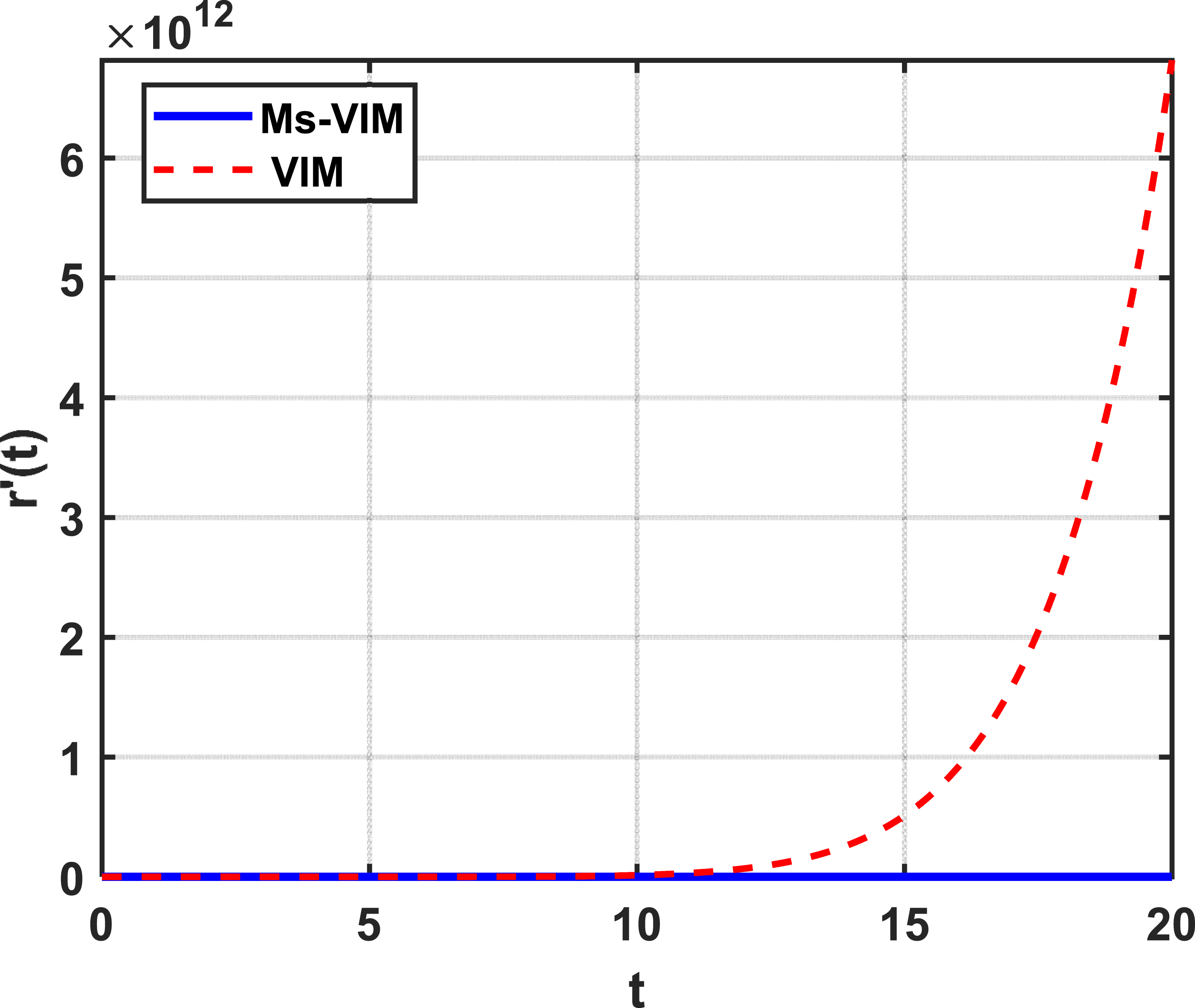
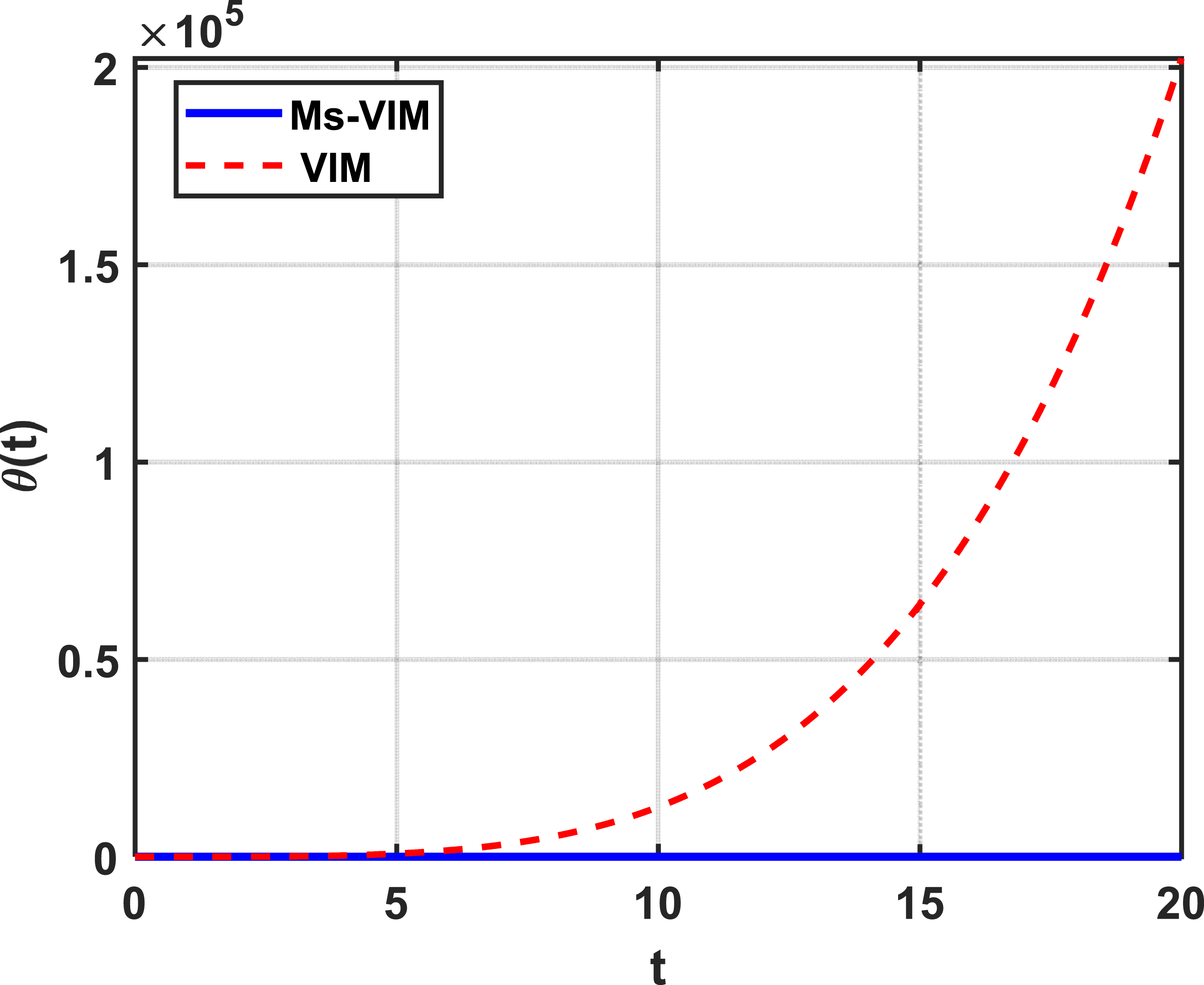
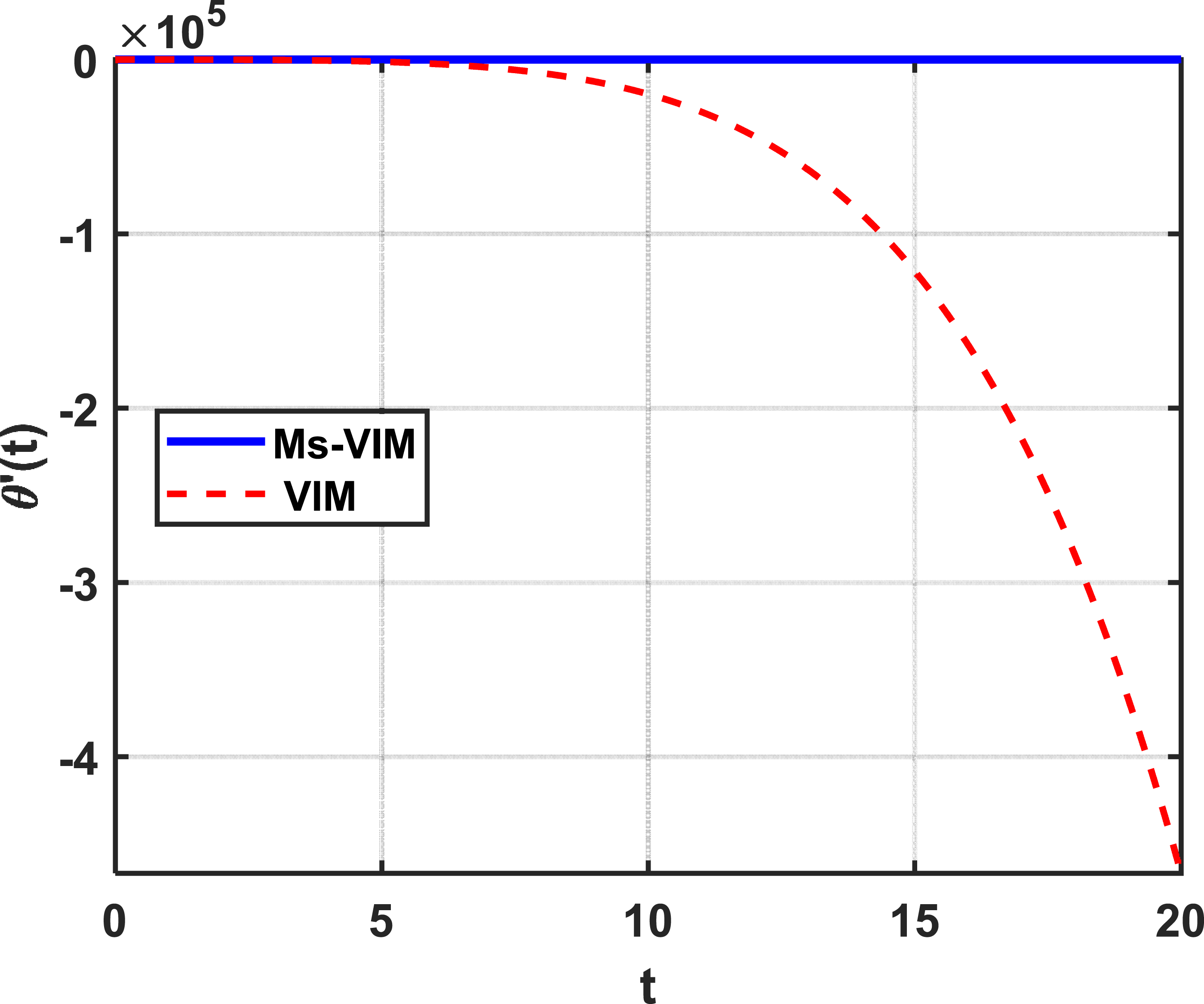
The dynamic behavior of the spring pendulum was examined through the use of the multi-stage variational iteration method (Ms-VIM). To establish the reliability of the analytical formulation, numerical simulations were carried out through the application of the classical fourth-order Runge-Kutta (RK4) method with identical parameter conditions. The simulations were performed on the time interval The system parameters were set as Figures 1–4 show the time histories of the state variables obtained by using the Ms-VIM method and the RK4 numerical method. The time history of the radial position of the end of the spring, The spring pendulum system. Time history of the radial displacement Time history of the radial velocity Time history of the angular displacement The time histories of the velocities of the end of the spring, The dynamical properties of the system are demonstrated using phase plots. A phase plot of the radial motion of the spring in the Time history of the angular displacement Phase portrait of the spring–pendulum system in the The accuracy of the proposed analytical technique was evaluated in a quantitative manner by computing the absolute differences between the Ms-VIM solution and the RK4 numerical solution for all of the state variables. Physically, the results obtained show the strong nonlinear coupling between the radial and angular motions of the spring-pendulum system. The effective pendulum length is continuously modified by the periodic extension and contraction of the spring, which affects the angular oscillation characteristics. This interaction leads to amplitude modulation and small frequency changes of either mode of motion. Furthermore, in the conservative case, the closed phase trajectories correspond to bounded and dynamically stable oscillations, whereas in the damped case the spiral phase trajectories exhibit a constant energy dissipation and an approach to a stable equilibrium configuration. These results confirm the effectiveness of the proposed model for capturing the essential nonlinear dynamics of the spring–pendulum system. Figures 7–10 present the absolute error distributions for Phase portrait of the spring–pendulum system in the Absolute error distribution for the radial displacement Absolute error distribution for the radial displacement Absolute error distribution for the radial displacement As previously mentioned, in classical perturbation methods, truncation errors typically grow very quickly during long-time simulations due to the limitations on the convergence radius of the power series expansions. In contrast, the Ms-VIM method continuously updates the initial conditions at the start of each subinterval. Therefore, the Ms-VIM method prevents the propagation of the accumulated errors and maintains the accuracy of the analytical approximation for extended periods of time. The results of comparing the classical VIM and the multi-stage VIM for all of the state variables are presented in Figures 11–14. The classical VIM consistently diverges from the RK4 numerical solution as the time increases for all of the state variables. The primary cause of this divergence is the limited convergence radius of the perturbation series employed in the classical formulation. As the time interval of integration is increased, truncation and phase errors accumulate and lead to noticeable discrepancies. Conversely, the Ms-VIM solutions remain in excellent agreement with the RK4 numerical solution for all of the state variables throughout the entire time interval. The subdivision of the time domain into smaller subintervals ensures that the local analytical approximation always remains within its convergence region. Therefore, the comparisons clearly demonstrate that the multi-stage implementation significantly enhances the long-term stability and accuracy of the variational iteration method. Absolute error distribution for the radial displacement Comparison between the multi-stage variational iteration method (Ms-VIM) and the classical variational iteration method (VIM) for the radial displacement Comparison between the multi-stage variational iteration method (Ms-VIM) and the classical variational iteration method (VIM) for the radial displacement Comparison between the multi-stage variational iteration method (Ms-VIM) and the classical variational iteration method (VIM) for the radial displacement Physically, the results obtained in this study emphasize the inherent coupling between the radial and angular motions of the spring pendulum. The oscillatory radial extension of the spring modifies the effective length of the pendulum, which in turn modifies the angular motion of the pendulum. This mutual interaction produces nonlinear effects in the modulations of both the displacement and velocity responses of the system. Nevertheless, despite the nonlinear coupling between the radial and angular motions, the system maintains bounded oscillations and closed phase trajectories, thereby establishing that the equilibrium configuration of the system remains dynamically stable under the specified parameter conditions.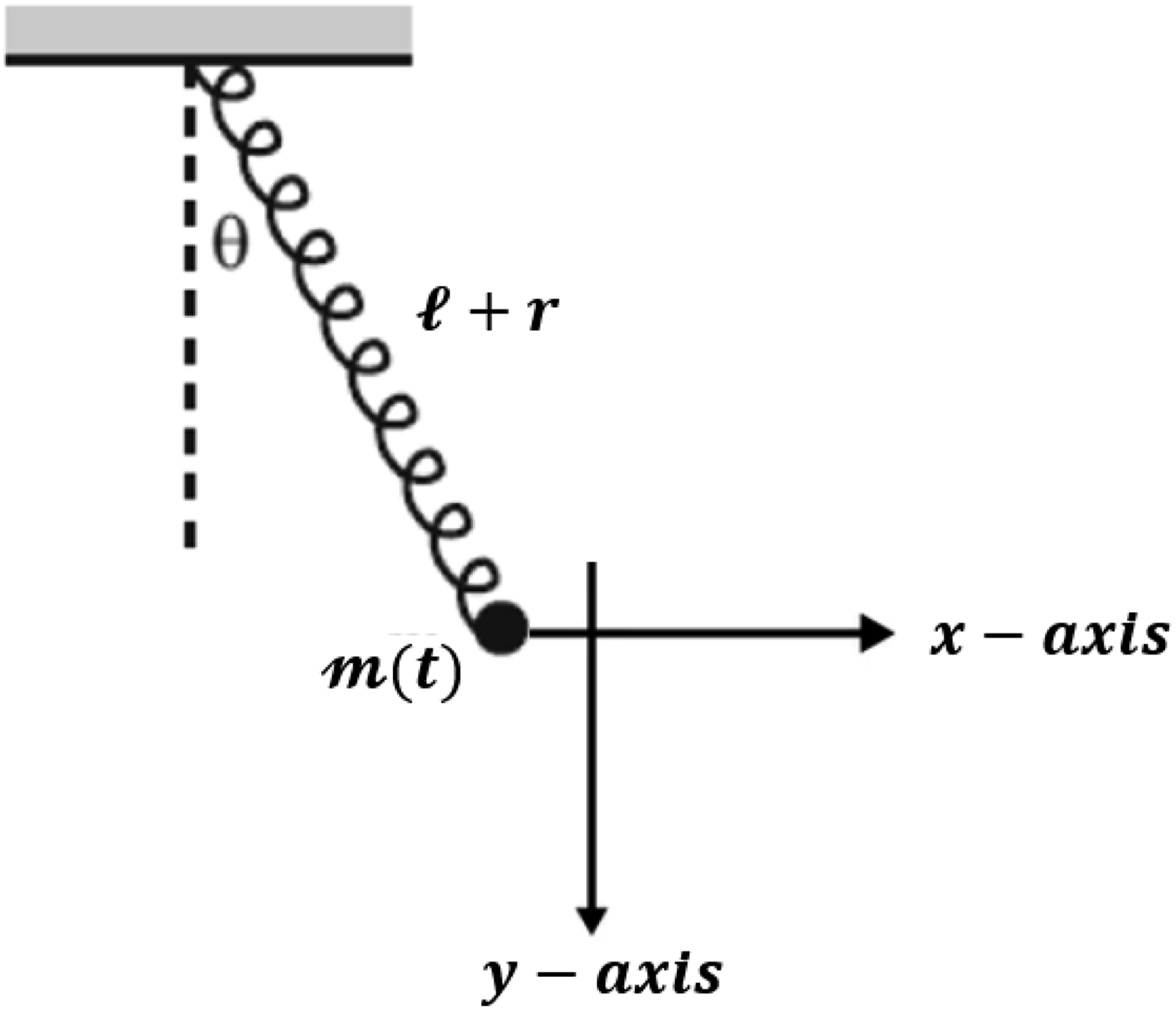
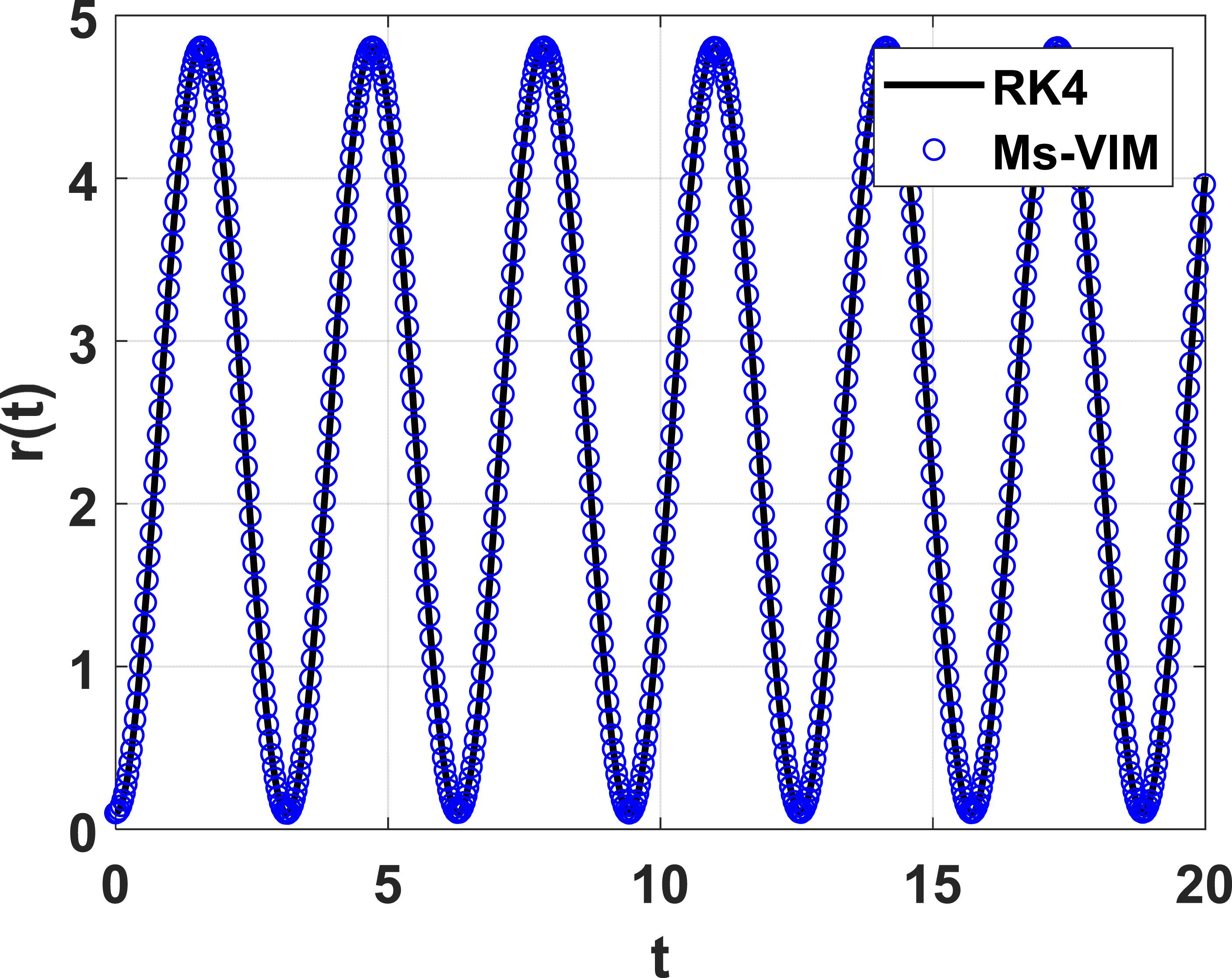
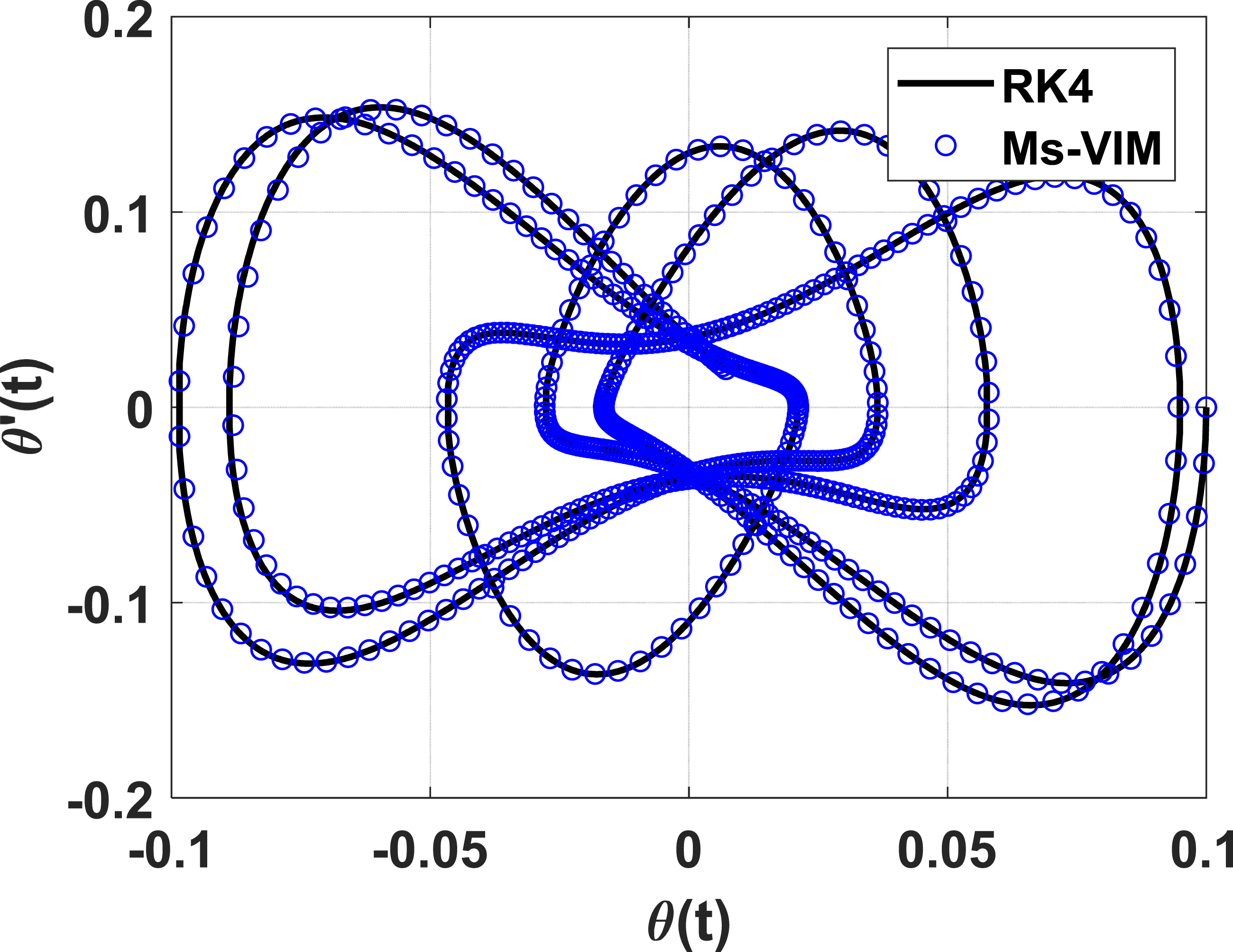
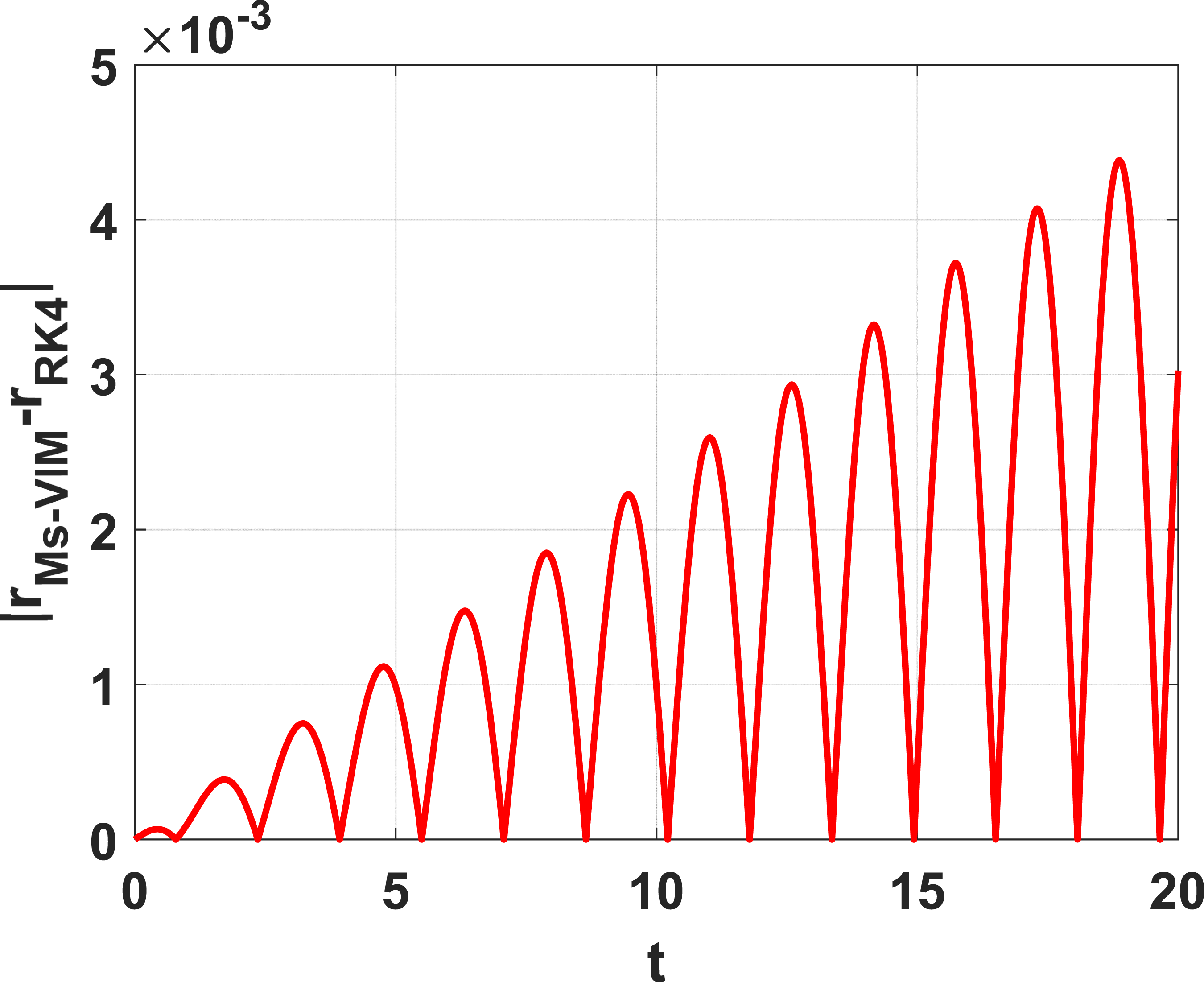
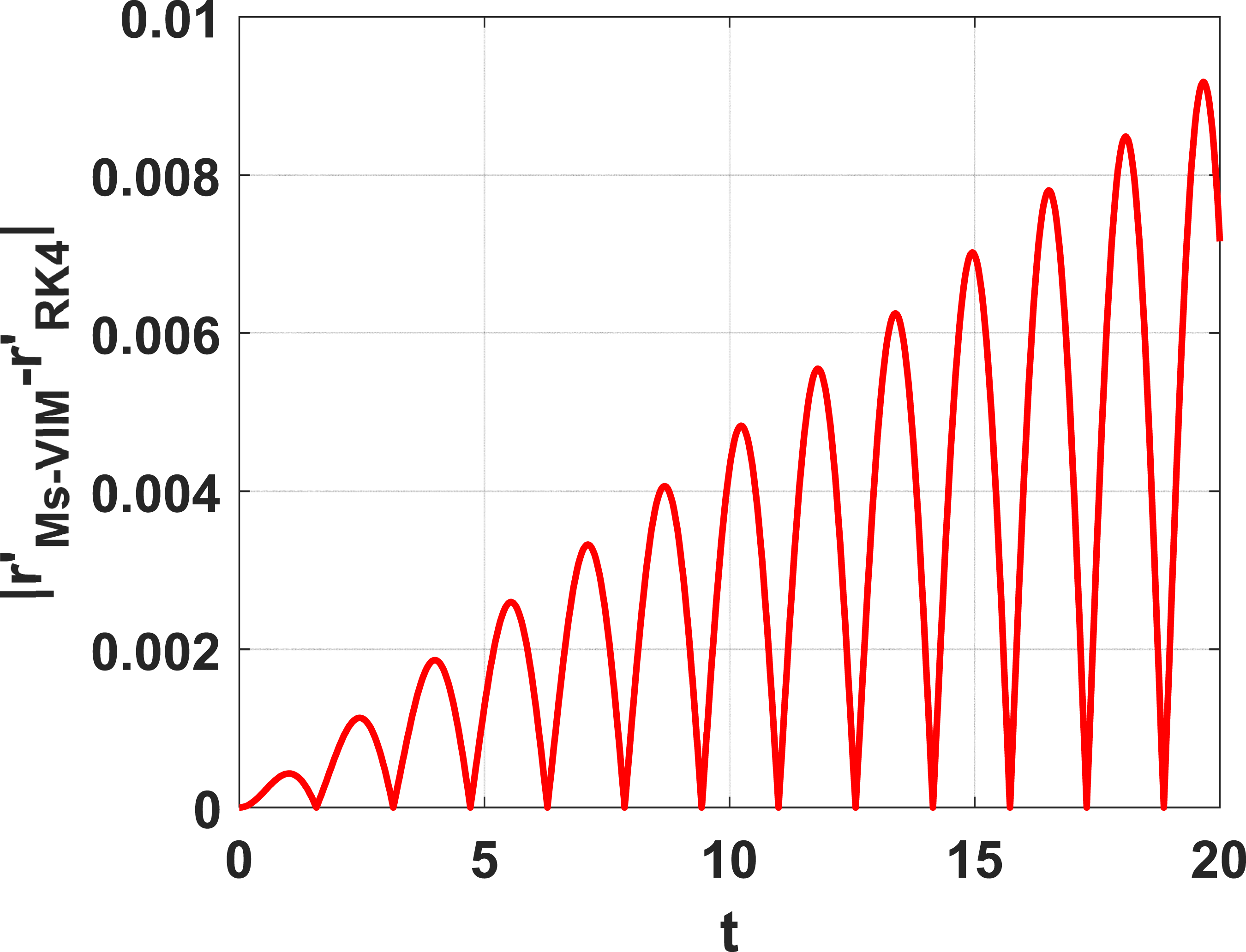
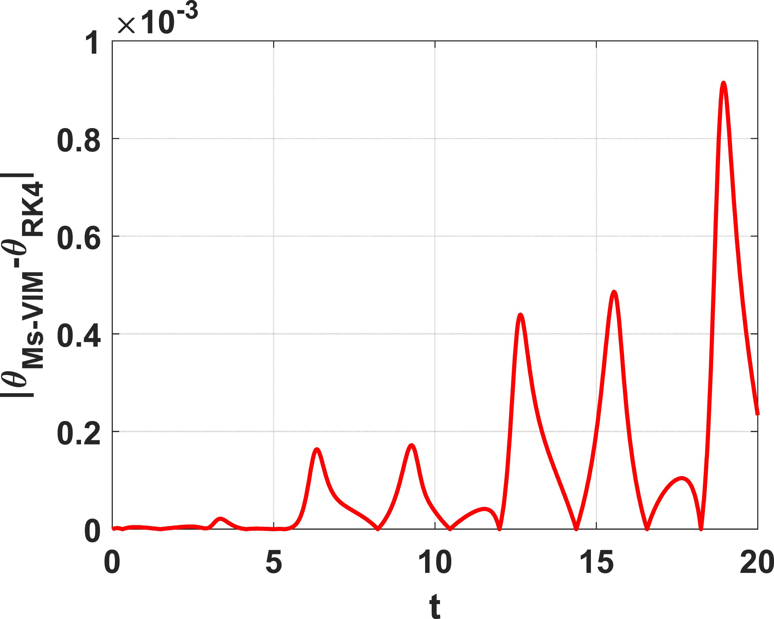
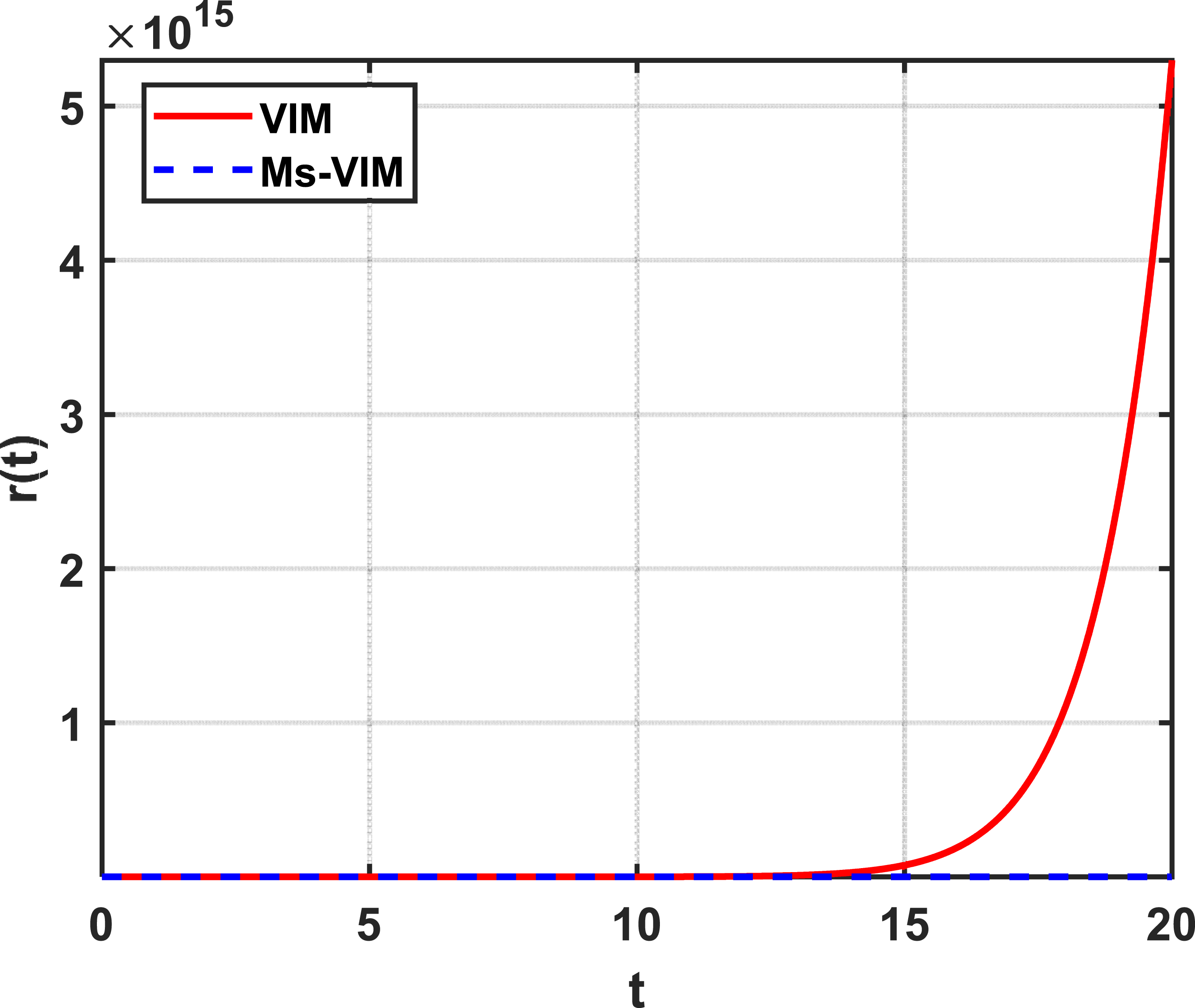
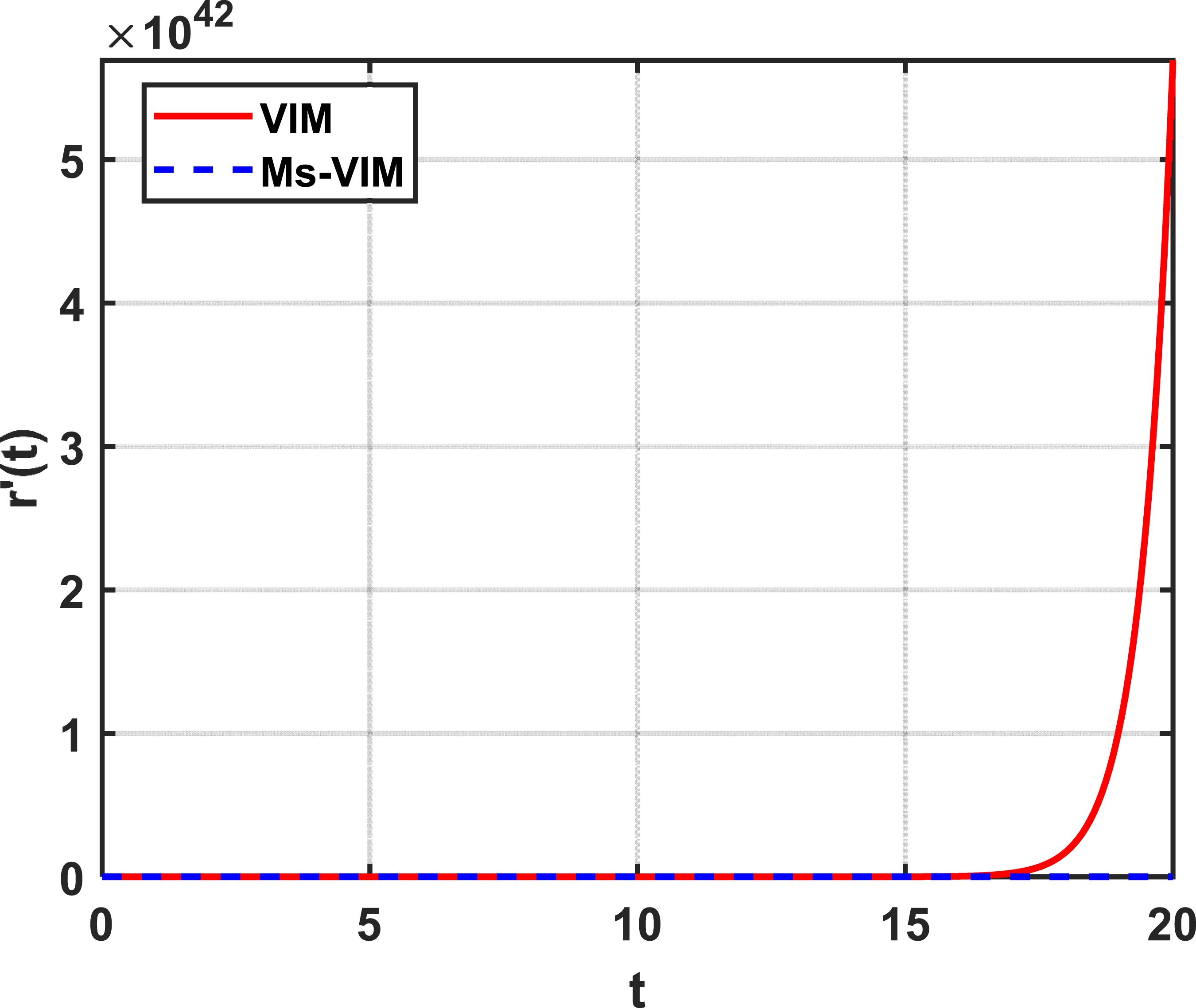
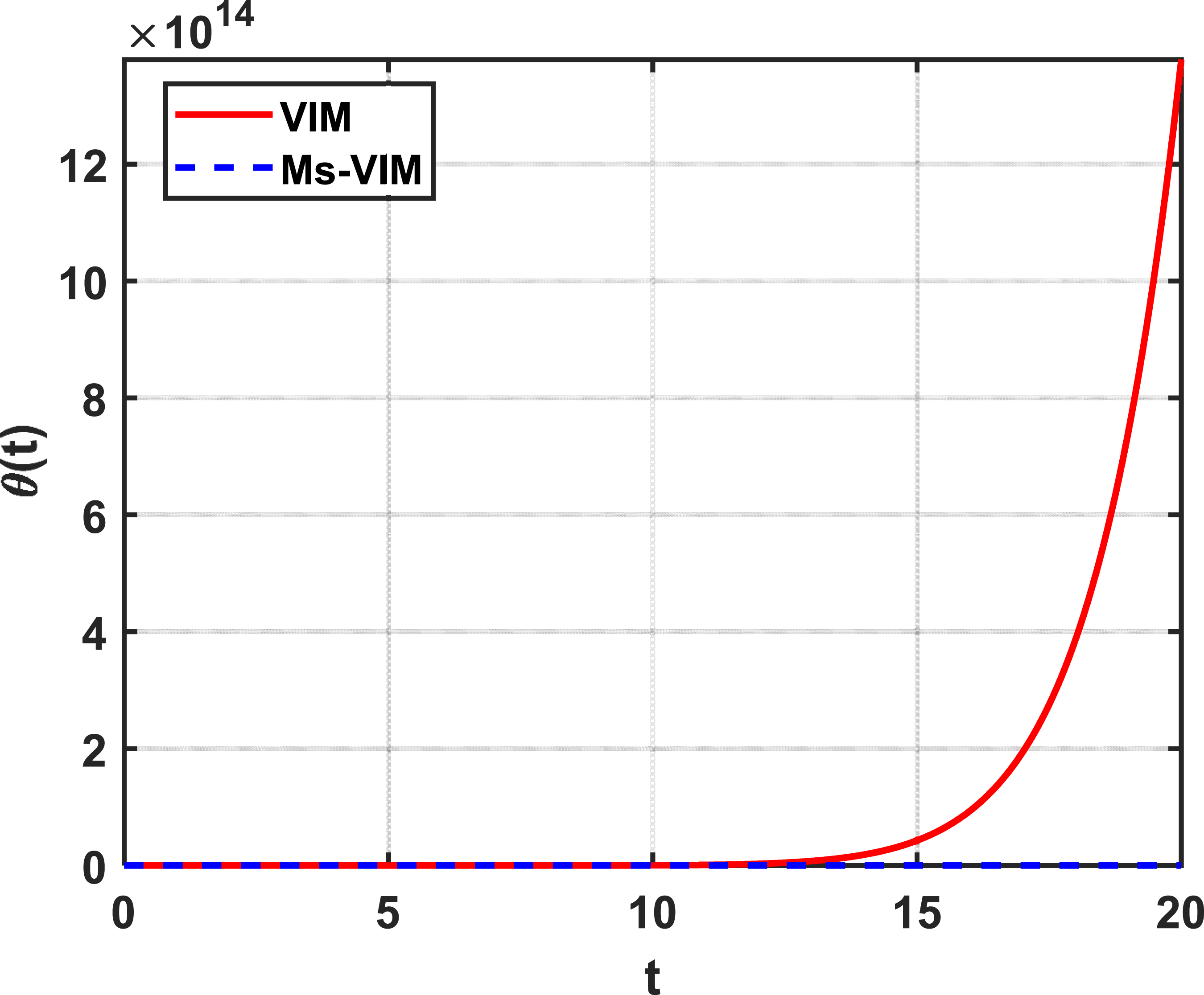
In the second instance, we study the impact of viscous damping on the dynamics of the spring pendulum system. Viscous resistances are included by means of the Rayleigh dissipation function. Energy loss, which occurs due to both radial spring deformation and the rotation of the pendulum, is represented by the two damping coefficients c (r)and cθ. We use the same computational framework as in Case 1. To ensure that our analytical solutions are reliable and accurate, we compare the analytical solution obtained by means of the multi-stage variational iteration method (Ms-VIM) to the numerical solution obtained by means of the fourth-order Runge-Kutta (RK4) method. The time-histories of the radial displacement r(t), the angular displacement Comparison between the multi-stage variational iteration method (Ms-VIM) and the classical variational iteration method (VIM) for the radial displacement Time history of the radial displacement Time history of the radial velocity Time history of the angular displacement The angular displacement The velocity responses The effect of damping on the stability of the system is further illustrated in Figures 19 and 20, which depict the phase portraits of the damped system. The phase trajectory in the Time history of the angular displacement Phase portrait of the spring–pendulum system in the To evaluate the accuracy of the analytical Ms-VIM solutions, we computed the absolute error with respect to the numerical RK4 solution. The absolute errors related to the Even in the presence of damping, which introduces additional nonlinear terms into the equations of motion, the Ms-VIM method provides stable and accurate predictions. The lack of significant error accumulation, which would have occurred if the errors had accumulated over time, further demonstrates the efficiency of the multi-stage formulation in limiting the truncation errors over long simulation times. Phase portrait of the spring–pendulum system in the Absolute error distribution for the radial displacement Absolute error distribution for the radial displacement Absolute error distribution for the radial displacement A comparative analysis of the results obtained by the classical VIM and the Ms-VIM for all four state variables is provided in Figures 25–28. The classical VIM solution starts to deviate from the numerical solution over time. This deviation can be attributed to the limited convergence radius of the perturbation series employed in the classical formulation. Over time, truncation and phase errors accumulate and lead to a degradation of the accuracy of the classical approach. On the contrary, the Ms-VIM results remain virtually identical to the RK4 numerical solutions throughout the entire simulation period.(Figure 29) The subdivision of the entire time domain into smaller subdomains ensures that the analytical series remains inside its convergence zone. Thus, the multi-stage approach significantly enhances the long-term stability and reliability of the analytical solution. Absolute error distribution for the radial displacement Comparison between the multi-stage variational iteration method (Ms-VIM) and the classical variational iteration method (VIM) for the radial displacement Comparison between the multi-stage variational iteration method (Ms-VIM) and the classical variational iteration method (VIM) for the radial displacement Comparison between the multi-stage variational iteration method (Ms-VIM) and the classical variational iteration method (VIM) for the radial displacement Comparison between the multi-stage variational iteration method (Ms-VIM) and the classical variational iteration method (VIM) for the radial displacement Physically, the results demonstrate how damping influences the nonlinear dynamics of the spring pendulum system. The presence of viscous forces removes energy continuously from the system, so that the oscillation amplitudes of both radial and angular motions decrease over time. Although the nonlinear coupling between the radial extension of the spring and the angular displacement of the pendulum exists, the system behaves stably and ultimately tends toward an equilibrium state. The spiral shape of the phase trajectories demonstrates that the system moves toward a dynamically stable configuration without showing chaotic or unstable behavior under the given parameter conditions.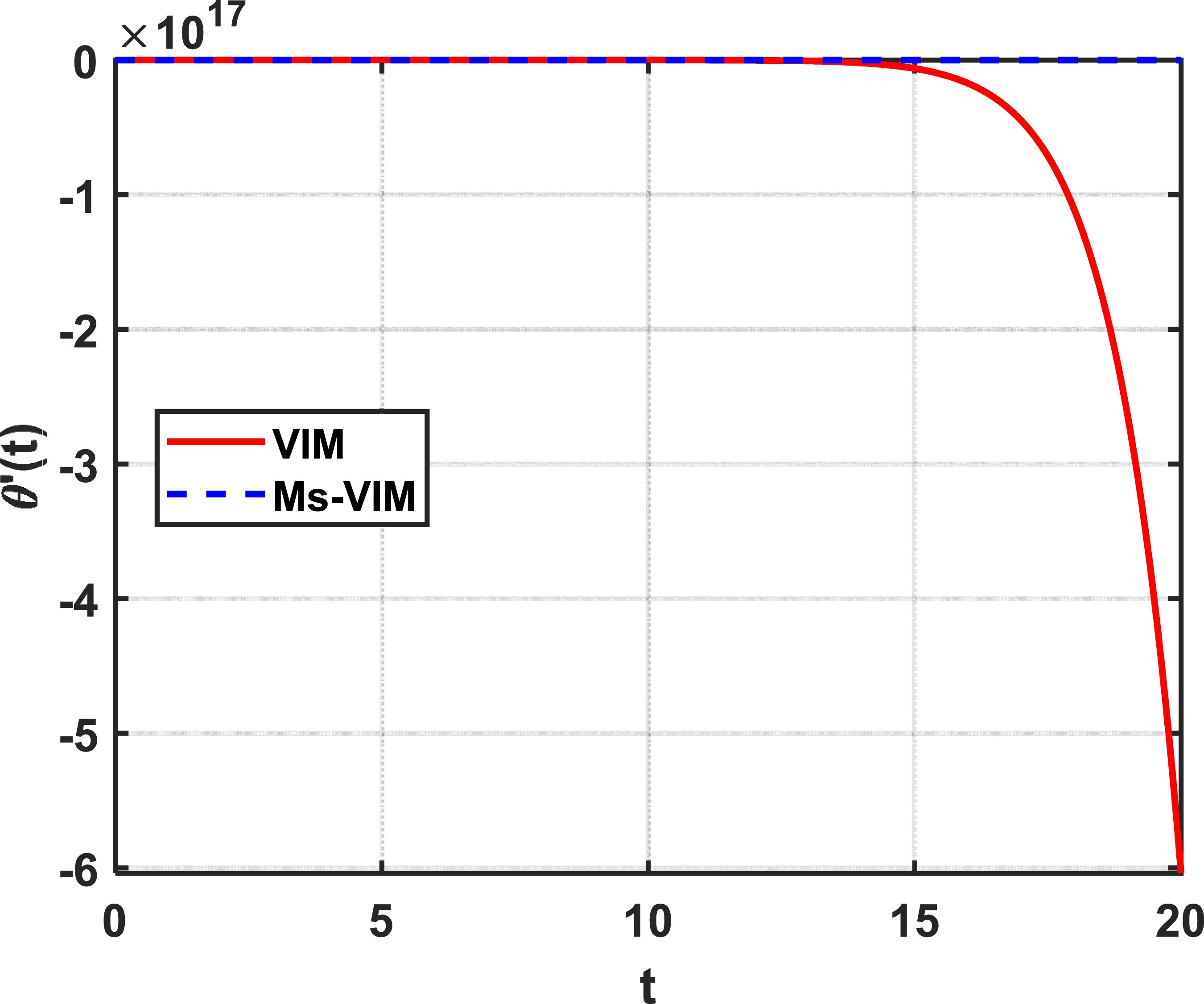
4.1. Sensitivity and stability analysis
To further investigate the dynamical behavior of the spring–pendulum system, a stability and sensitivity analysis was carried out for both the conservative and damped cases. The phase portraits presented in Figures 5, 6, 19 and 20 provide important information regarding the stability of the motion. In the conservative case, the trajectories form closed bounded curves around the equilibrium position, which indicates stable periodic oscillations of the system. The absence of diverging trajectories confirms that the nonlinear coupling between the radial and angular motions does not lead to instability within the considered parameter range.
For the damped system, the phase trajectories gradually spiral toward the equilibrium point. This behavior is expected due to the presence of viscous damping, which continuously removes energy from the system. As time increases, the amplitudes of both the radial and angular oscillations decrease until the motion approaches a stable equilibrium configuration. Therefore, the damped system can be considered asymptotically stable.
A sensitivity analysis was also performed by introducing small perturbations in the initial conditions and damping coefficients. The numerical results showed that moderate variations in these parameters produce only small changes in the displacement and velocity responses. Although the nonlinear interaction between the radial and angular motions slightly modifies the oscillation amplitudes and frequencies, the qualitative behavior of the system remains unchanged. No unstable or chaotic behavior was observed for the selected parameters and initial conditions.
These observations demonstrate that the proposed spring–pendulum model possesses stable nonlinear dynamics and that the Ms-VIM method remains reliable and accurate even when small perturbations are introduced into the system parameters.
5. Conclusion
This research has been based on development of a numerical/analytical solution technique which allows the investigation into the nonlinear dynamics of a spring pendulum of constant mass. A common application for this type of device is found in engineering examples including; cranes, robotic manipulator arms and vibration control devices. Using the Lagrangian variational formulation the authors have formulated the governing equations describing the coupled motion of both the radially and angularly moving components of the device. The results show that due to the nonlinear coupling between the two modes of motion there are amplitude modulation and nonlinear frequency shifts that can occur in the motion of the system and can not be modeled by the classical linear approximation techniques.
The time domain response and the phase plane trajectories of the system indicate a stable oscillating behavior over the entire range of parameters examined and the bounded and closed phase plane trajectories indicate the dynamic stability of the system. The Ms-VIM was able to provide reliable semi-analytical solutions for the system at a significant reduction in computational cost compared to other numerical methods including the RK4 method. Due to the fact that the authors have validated their method against the RK4 method they have shown that the proposed method will provide a useful tool for engineers when designing and modeling nonlinear spring-pendulum systems. Nevertheless, the Ms-VIM has some limitations: it requires careful selection of subinterval size to balance accuracy and computational cost, and the derivation of Lagrange multipliers may become difficult for highly complex nonlinear systems.
The Ms-VIM can be extended to multi-degree-of-freedom systems and parametrically excited oscillators, where classical perturbation methods often struggle. Future work may also explore adaptive subinterval sizing for improved computational efficiency.
Another promising extension is to formulate the spring-pendulum system in fractal or fractional space, which can capture memory effects and complex damping mechanisms more accurately. Recent advances in fractal calculus and fractional modelling (see e.g., recent issues of Fractals and Chaos, Solitons & Fractals) offer powerful tools for such investigations. This remains an important direction for future work.
Footnotes
Acknowledgment
The authors Rania Wannan, and Jihad Asad would like to thank Palestine Technical University- Kadoorie for supporting them financially during this research.

Funding
The authors received no financial support for the research, authorship, and/or publication of this article.
Declaration of conflicting interests
The authors declared no potential conflicts of interest with respect to the research, authorship, and/or publication of this article.