
Abstract
Modelling based on the Birnbaum–Saunders distribution has received considerable attention in recent years. In this article, we introduce a new approach for Birnbaum–Saunders regression models, which allows us to analyze data in their original scale and to model non-constant variance. In addition, we propose four types of residuals for these models and conduct a simulation study to establish which of them has a better performance. Moreover, we develop methods of local influence by calculating the normal curvatures under different perturbation schemes. Finally, we perform a statistical analysis with real data by using the approach proposed in the article. This analysis shows the potentiality of our proposal.
Keywords
1 Introduction
Birnbaum and Saunders (1969a, 1969b) proposed a statistical model for fatigue life of structures under cyclic stress. Based on a setting that shows that the failures originate from the development of a dominant crack produced by cumulative stress, they derived the Birnbaum–Saunders (BS) distribution.
The BS distribution has received considerable attention in recent years, due to its theoretical arguments associated with cumulative damage processes, its properties and its relation with the normal distribution. Specifically, the amount of cumulative damage that allows the BS distribution to be generated is assumed to follow a normal distribution. This model corresponds to a unimodal, positively skewed, two-parameter distribution and with positive support. Over the past decades, theoretical, methodological and practical aspects of the BS model have been largely studied; see, e.g., Johnson et al. (1995, pp. 651–63) for a general scope, and Owen and Padgett (2000), Guiraud et al. (2009) and Ho (2012) for applications in engineering. Novel practical applications of this model have been recently considered in areas different from engineering, which include business, environment and medicine; see, e.g., Leiva et al. (2007, 2008, 2009, 2010, 2011, 2012), Barros et al. (2008), Bhatti (2010), Vilca et al. (2010, 2011), Paula et al. (2012), Ferreira et al. (2012) and Marchant et al. (2013a, 2013b). Some extensions and generalizations of the BS distribution are attributed to Díaz-García and Leiva (2005), Vilca and Leiva (2006), Gómez et al. (2009), Kotz et al. (2010), Balakrishnan et al. (2011), Caro-Lopera et al. (2012) and Fierro et al. (2013).
A random variable Y follows a BS distribution with shape parameter α > 0 and scale parameter > 0, denoted by Y ∼ BS(α, ), if its probability density function (PDF) takes the form

In addition, ϱ is the median of the distribution of Y, 1/Y ∼ BS(α,1/ϱ) and bY ∼ BS (α,bϱ), if b > 0. The mean of Y is E[Y] = ϱ[1 + α2/2] and its variance is Var[Y] = [αϱ]2 [1 + 5α2/4].
Statistical modelling based on BS distributions has considerably attracted the attention of a number of researchers. Rieck and Nedelman (1991) were the pioneers in this line. They defined that if Y ∼ BS(α, ϱ), then V = log(Y) follows a log-BS distribution with shape parameter α and location parameter γ = log(ϱ) ∈ ℝ, denoted by V ∼ log-BS(α, γ). They proposed log-linear regression models based on the log-BS distribution and applied them to fatigue data, whereas Galea et al. (2004) and Xie and Wei (2007) developed several diagnostic tools for this model. Leiva et al. (2007) formulated BS log-linear regression models and their diagnostics, and applied them to survival data of patients with blood cell cancer. Barros et al. (2008) assumed that the cumulative damage follows a Student-t distribution and then introduced BS-t log-linear regression models and their diagnostics, and applied them to survival data of patients with lung cancer. They showed that the maximum likelihood (ML) estimates for the parameters of this model are robust against outliers, which was conjectured by deviance and martingale residuals. This conjecture was mathematically formalized by Paula et al. (2012), who in this work applied BS-t log-linear models to insurance data. Lemonte and Cordeiro (2009) proposed BS non-linear regression models, generalizing the proposal of Rieck and Nedelman (1991). Lemonte and Patriota (2011) and Vanegas et al. (2012) performed diagnostic procedures for these non-linear models. For all of these regression models, the original response must be transformed to a logarithmic scale, which could provoke a reduction of the power of the study and difficulties of interpretation; see Huang and Qu (2006). In addition, although in this scale one is modelling the mean, say γ = log(ϱ), in the original scale one is modelling ϱ = exp(γ), which, in the BS case, as aforementioned, corresponds to the median. This issue could make sense when lifetime data are modelled, but if we are analyzing data in other areas, such as business, it makes more statistical sense to model the mean. Recently, Santos-Neto et al. (2012) proposed new parameterizations for the BS distribution. One of them allows us to rely the BS distribution on the mean, such as Ferrari and Cribari-Neto (2004) did, which is a similar idea to that of generalized linear models (GLM), but based on the BS distribution that does not belong to the exponential family.
The objective of this article is to develop a new approach based on BS regression models following the line of GLM. In this context, the mean response is related to the linear predictor through a link function. This linear predictor encompasses regressors and unknown parameters. Unlike the existing BS regression models at present, the new approach that we propose models the data in their original scale, because it is based on the population mean.
The remainder of the article unfolds as follows. In Section 2, we introduce a reparameterization of the BS distribution that allows us to postulate a new approach. In Section 3, we define new BS regression models, calculate their corresponding score function and develop an iterative process to estimate their parameters. In Section 4, we perform a diagnostic analysis based on normal curvatures useful for a local influence analysis, whereas in Section 5, we analyze the concept of generalized leverage (GL) for the new approach. In Section 6, we propose four types of residuals for the new BS regression models. In Section 7, we carry out Monte Carlo simulations to study the behaviour of these residuals. In Section 8, we show the potentiality of the new approach through an application with real data. Finally, in Section 9, we sketch some conclusions obtained throughout this work.
2 A BS distribution parameterized by its mean
One new parameterization of the BS distribution proposed by Santos-Neto et al. (2012) is indexed by the parameters µ and δ, where µ > 0 is a scale parameter and the mean of the distribution, whereas δ > 0 is a shape and precision parameter. Based on this parameterization, the PDF of Y is given by

In this case, we use the notation Y ∼ BS(µ, δ). The mean and variance of Y are given by E[Y] = µ and Var[Y] = µ2/φ, respectively, where φ = [δ + 1]2/[2δ + 5], such that, as mentioned, δ can be interpreted as a precision parameter, that is, for fixed values of µ, when δ → ∞, the variance of Y tends to zero. Also, for fixed µ, if δ → 0, then Var[Y] → 5µ2. We can see that Var[Y] = µ2/φ is similar to the variance function of the gamma distribution, in which case the variance has a quadratic relation with its mean. It is also possible to show that bY ∼ BS (bµ, δ), with b > 0, and 1/Y ∼ BS(µ*, δ), where µ*= [δ + 1]/[δµ].
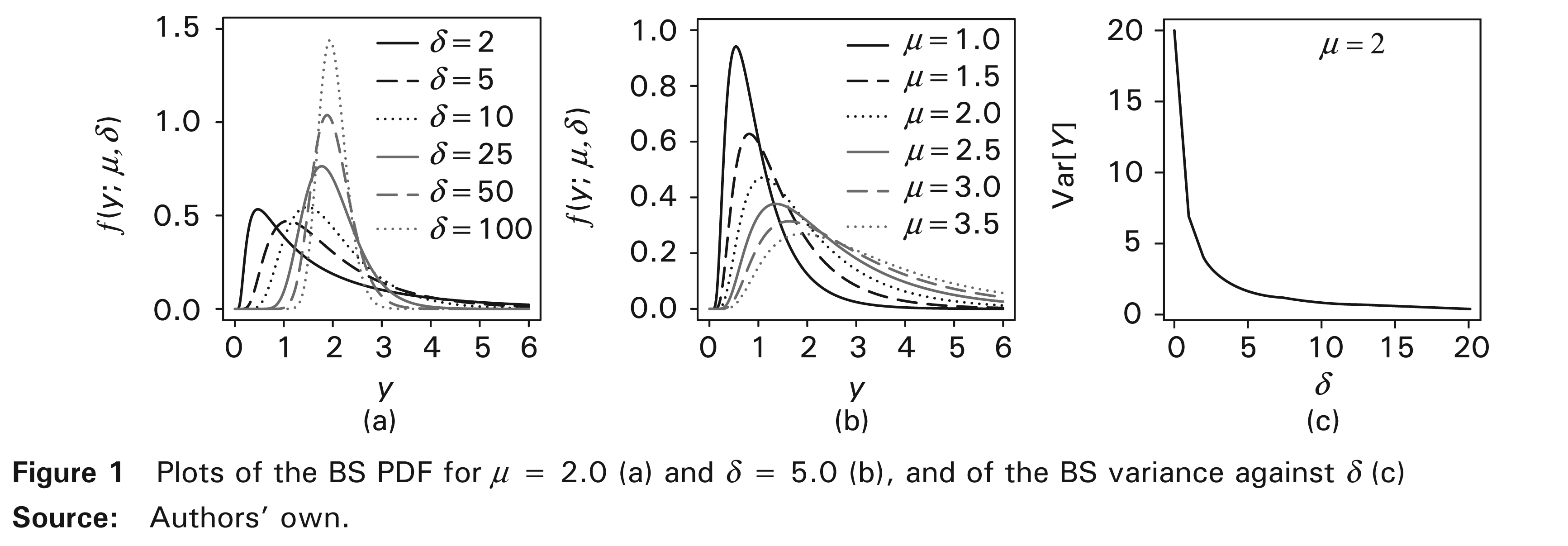
Figure 1 displays some shapes of the PDF of Y ∼ BS(µ, δ) given in (2.1). From Figure 1(a), note that the parameter δ controls the skewness and kurtosis of the distribution. It is also possible to note that, as δ increases, the corresponding PDF is more concentrated around the mean and, therefore, the variability decreases. From Figure 1(b), note that the parameter µ alters the scale of the distribution and, as it increases, the variability increases too. Finally, from Figure 1(c), note that the variance tends to 20, when µ = 2 and δ → 0, whereas it tends to zero, as δ → ∞.
3 Modelling and estimation
Let Y1, …, Yn be independent random variables, where Yi ∼ BS(µi, δ), for i = 1, …, n, and

where
We have that Var[Yi] is a function of µi and, consequently, of the regressors
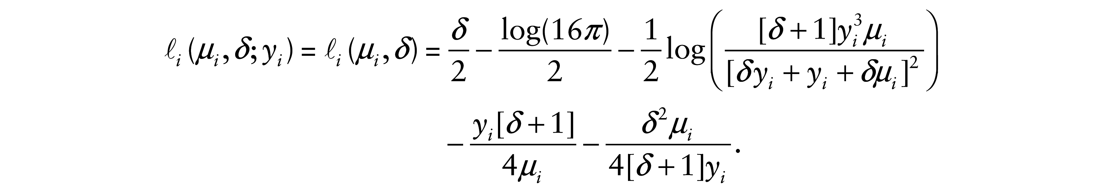
The log-likelihood function of the model given in (3.1) for
The score functions for βj, with j = 1, …, p, and δ are, respectively, given by
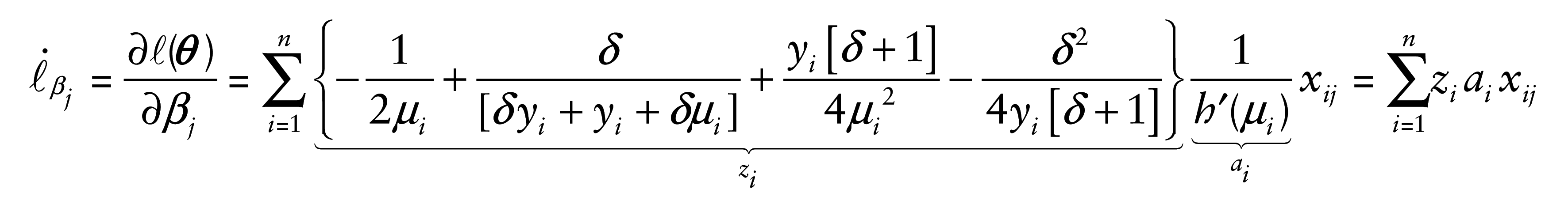
and
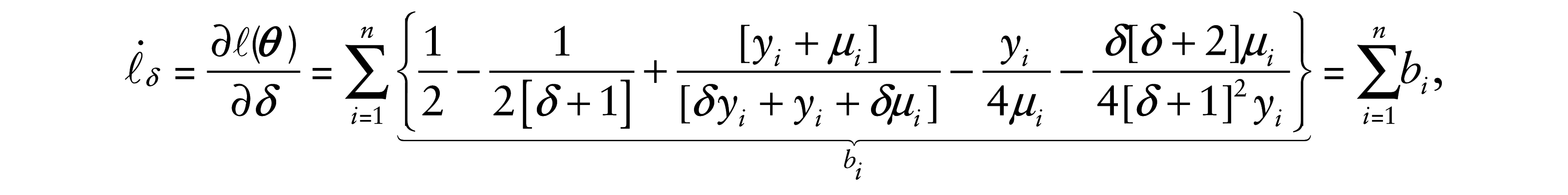
where h′ is the derivative of h. Then, in matrix form, we have

where
In order to estimate the model parameters by the ML method, we solve the equation
The algorithm for estimating

where

with
Therefore, the inverse of
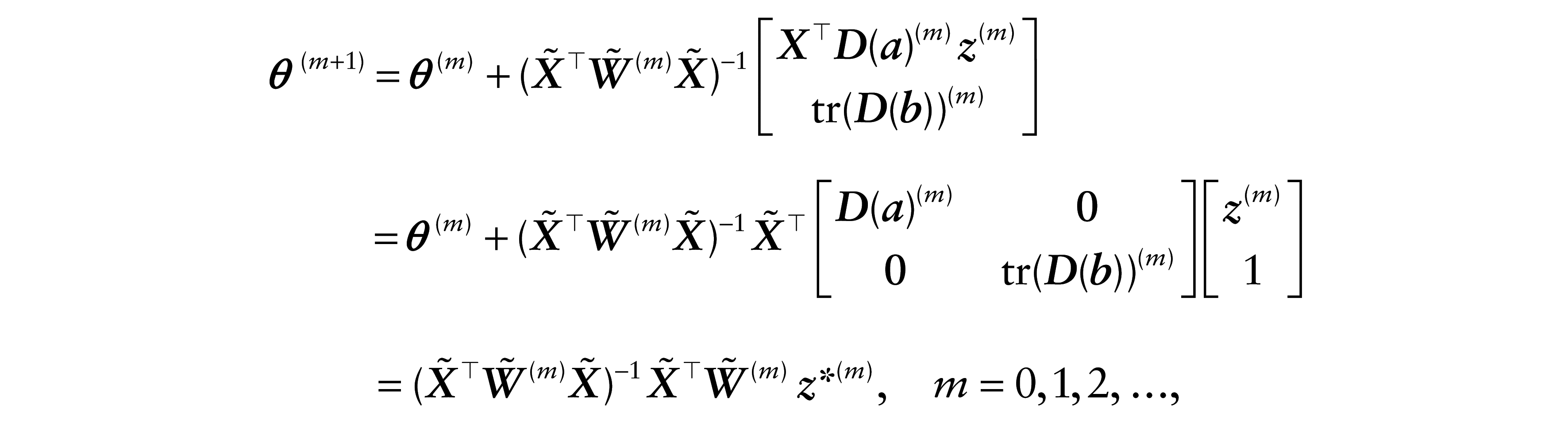
where

Note that
Under some regularity conditions (see Cox and Hinkley, 1974), the asymptotic distribution of
where
4 Local influence
The likelihood displacement is defined as

and
ω
(
For the model given in (3.1), the elements of

see Cook (1986). The index plot of
In case our interest is only on the vector

If our interest lies in studying the local influence on

Another important direction is
4.1 Case–weights perturbation
Let

where
4.2 Response perturbation
Consider now an additive perturbation on the ith response by making yi(ωi) = yi + ωi s(yi), where
and

where

and

4.3 Regressor perturbation
Consider now an additive perturbation on a particular continuous regressor, namely

and

where Δ

with

whereas, when j = t, it is given by

and

where ai is as given in (3.3) and
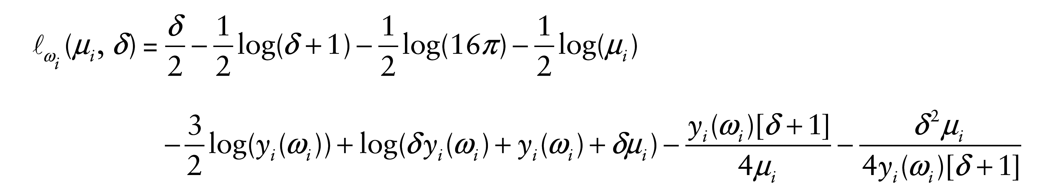
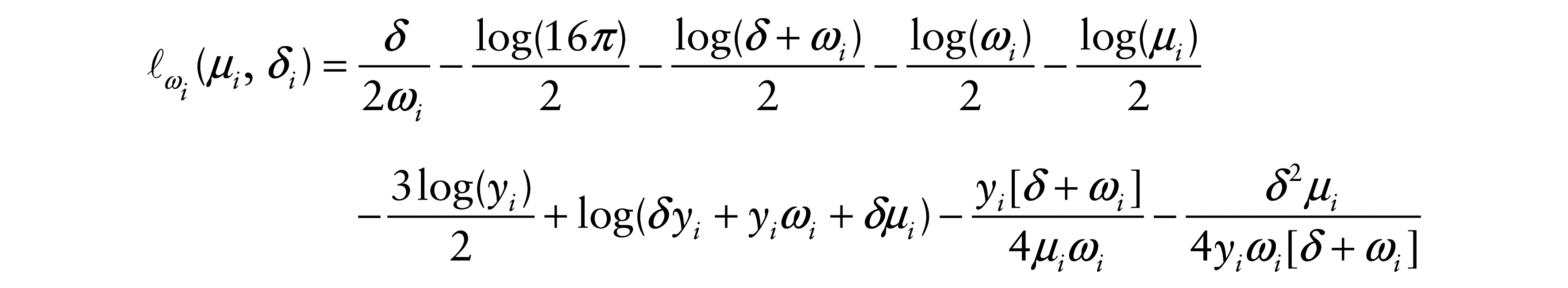
4.4 Perturbation on the precision parameter
We modify now the precision of the model given in (3.1) as δ
i
= δ/ωi, with ωi > 0, for i = 1, …, n, so that the precision of the perturbed model is non-constant across observations. In this case, the perturbed log-likelihood function is given by
and

where

and

5 Generalized leverage
The study of leverage points has as objective to evaluate the influence of the observed value of the response yi on its own predicted value

where

and

is the GL for the vector of parameters

6 Residual analysis
We propose four types of residuals for the BS regression models defined in Section 3.
6.1 First type of residual
This residual is based on the difference

where φ and µi are as given in (2.1) and (3.1), respectively.
6.2 Second type of residual
This second residual is based on the work proposed by Jørgensen (1984). Then, we have

where

and

with
6.3 Third type of residual
This third residual is based on the iterative process used in the estimation of the proposed model parameters. In the iterative process defined in (3.5), considering δ as known, we can write the expression of the estimate

where

where

6.4 Fourth type of residual
We have proposed three residuals for BS regression models. However, the most used residual in GLM is defined from the components of the deviance function. Assuming δ as fixed or known, we propose the deviance component (DC) residual for the BS regression model given in (3.1) as
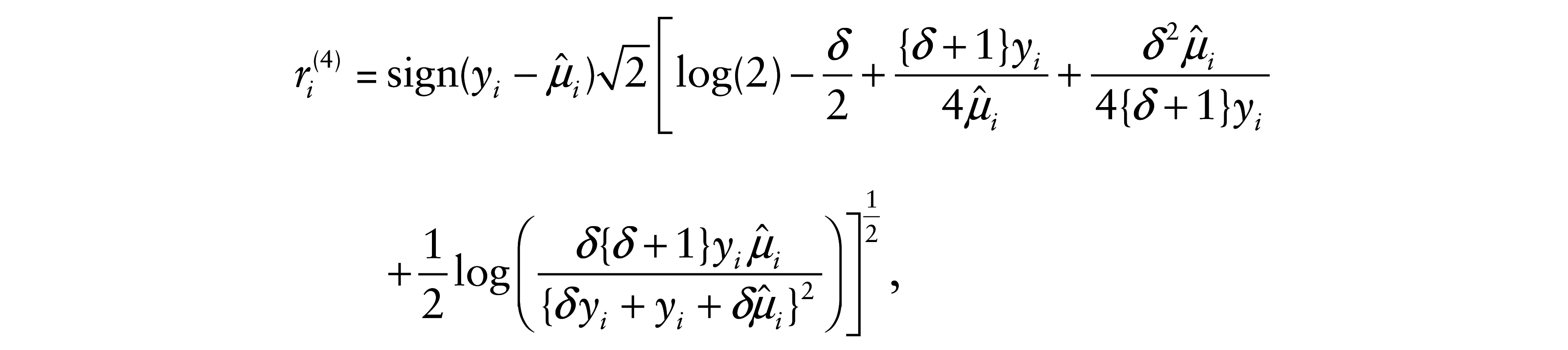
where
7 Simulation study
Based on the approach presented in this article, we develop a set of computational routines in R computer language; see http://www.R-project.org and Barros et al. (2009). These routines contain the functions bsreg, bsreg.fit, diagnostics.bs, envelope.bs, residuals and summary.bs, which are available to interested users upon request from the authors or from the website of the journal; see http://smj.sagepub.com.
We perform a simulation study to examine the distributions of the residuals r(1), r(2), r(3) and r(4) defined in (6.1), (6.2), (6.5) and (6.6), respectively. We use a BS regression model with link function
where the true values of the parameters are taken as β1 = 0.2, β2 = 0.5, and δ = 2 and δ = 25. In this study, we assume that the values of the regressor (xi) are obtained from a uniform distribution in the interval (0, 1). The number of Monte Carlo replications is 5000. Using the relation µi = exp(β1 β2xi), we obtain the values of µi. In each of the 5000 replications, we obtain the observations
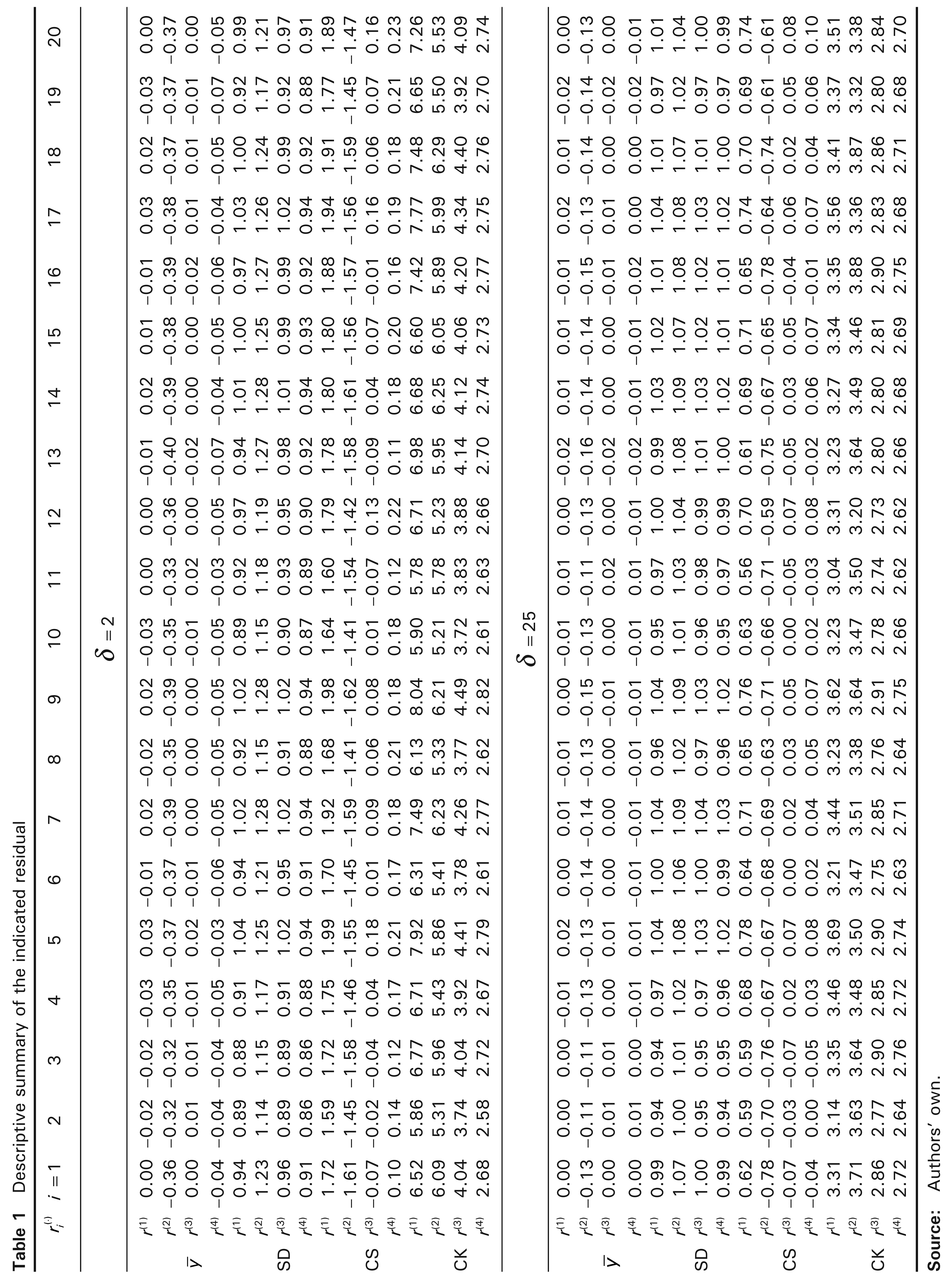
Table 1 displays descriptive statistics based on the mean (
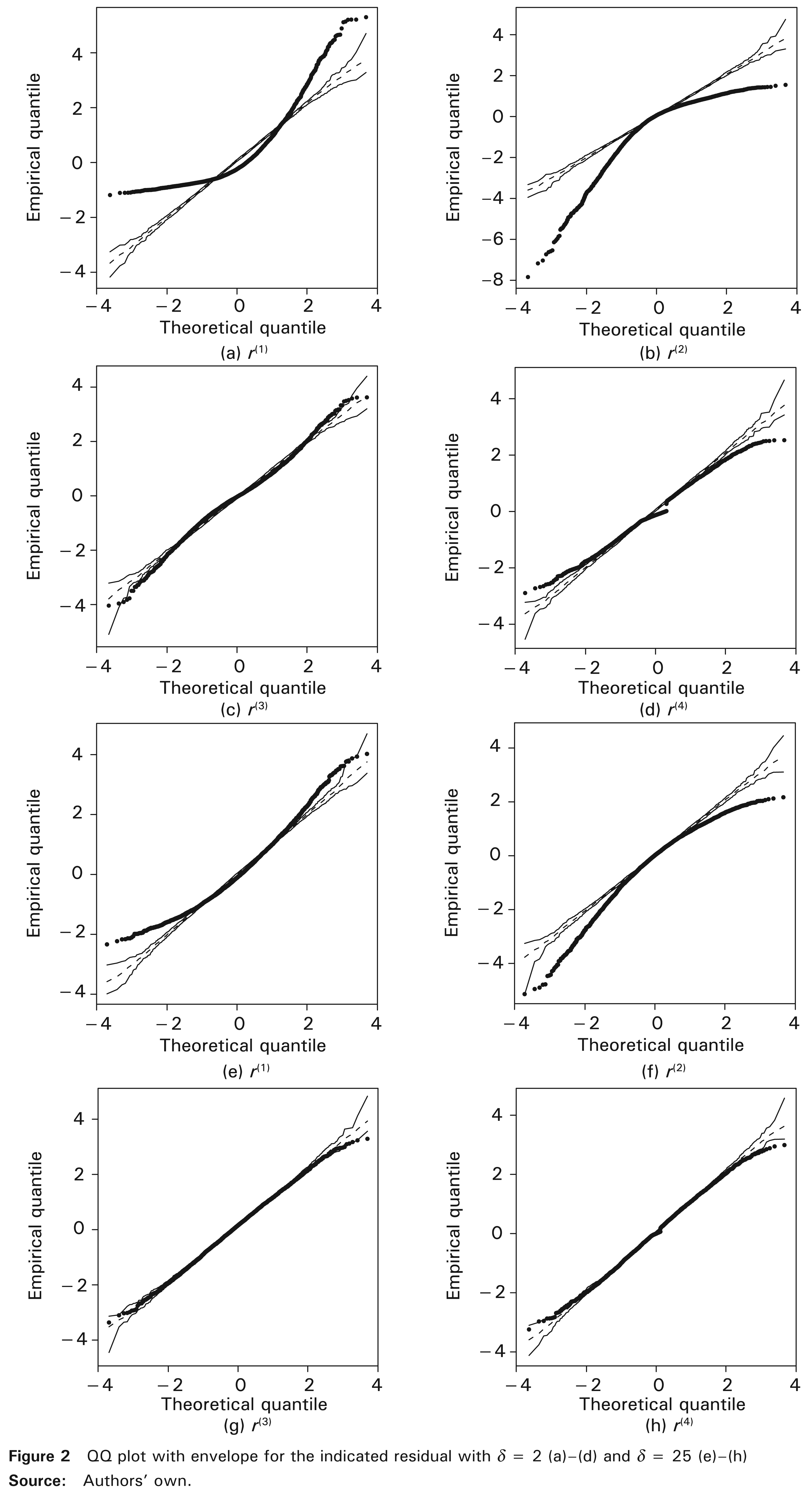
In order to graphically view the aspects detected in Table 1, we perform a comparison between the empirical (sample) distribution of the residuals and the standard normal distribution, by using a quantile against quantile (QQ) plot with simulated envelope; for more details about the QQ plot with envelope, see Atkinson (1985). Figure 2 presents eight QQ plots with simulated envelope, one for each 5000 residuals r(1), r(2), r(3), and r(4) and for each value of δ = 2 and δ = 25. Note that the QQ plots with simulated envelope of the residuals r(1) and r(2) are further away from the diagonal line and are outside the envelope. However, note that the residuals r(3) and r(4) present an approximately linear behaviour and have a good agreement with the normal distribution.
Descriptive summary of the indicated residual
8 Empirical application
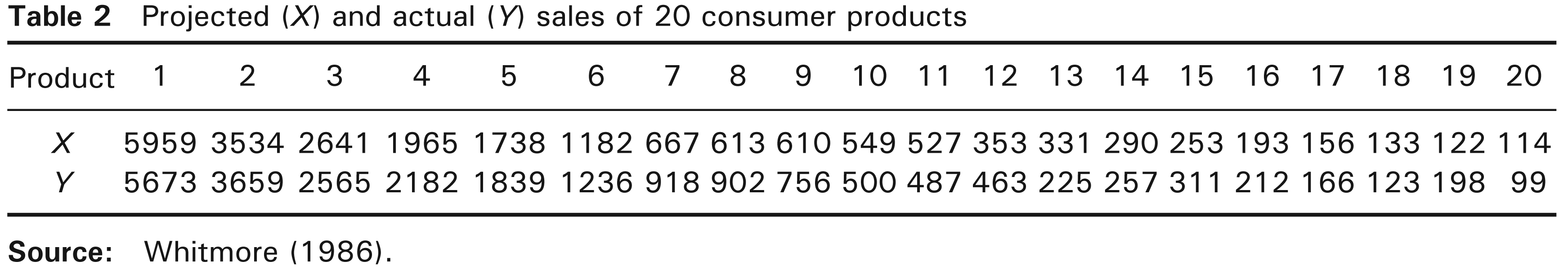
In the following, we analyze a real data set obtained by means of an R package called faraway, corresponding to the projected sales (regressor, xi, in M$) and actual sales (response variable, Yi, in M$) of 20 consumer products; for more details, see Whitmore (1986). These data can be accessed from the faraway package through the command data(cpd) and these are displayed in Table 2.
8.1 Exploratory data analysis
Table 3 provides a descriptive summary of the actual sales (in M$) that includes median (MD), mean (
Projected (X) and actual (Y) sales of 20 consumer products
statistics for the actual sales (in M$)
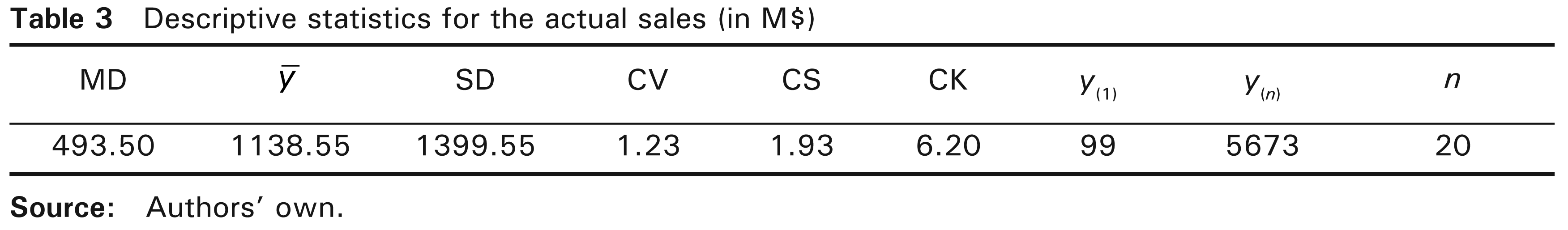
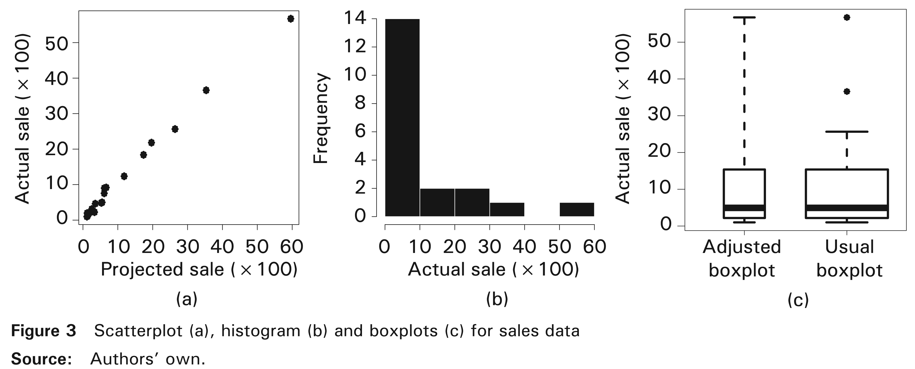
Based on Table 3 and Figure 3, we conduct an exploratory data analysis (EDA). First, from Figure 3(a), we see the actual sale for the ith product (yi) is linearly related to the ith projected sale (xi). In addition, this figure shows evidence that the line goes through the origin. Such an aspect is evaluated in Subsection 8.2. Also, from Figure 3(a), we observe the variability of the sales tends to increase as the sale values increase. This observation, which could be an indication of a non-constant variance in the data, is evaluated in Subsection 8.2. Second, from the histogram displayed in Figure 3(b), we note that the values of actual sales have an empirical distribution that is unimodal and positively skewed, whose values are concentrated primarily in the range [0, 1000]. Third, from Figure 3(c), we detect two atypical data by the usual boxplot, but the adjusted boxplot for asymmetric data do not show atypical data. Fourth, from Table 3 and Figure 3, we detect that the amplitude of the data suggests a high variability, which is corroborated by the high value of their CV (123%). In consequence, the BS regression model given in (3.1) may be suitable for describing the mean of the data, and the non-constant variance and asymmetry detected in these data. It is worth to highlight that none of the BS regression models postulated until now can simultaneously describe all these aspects.
8.2 Estimation and verification of assumptions
Based on the EDA performed in Subsection 8.1, we assume the response Yi ∼ BS(µi , δ) for sale data. Then, the systematic component of the regression model on the mean, by using the identity link function, is expressed as
with β1 and β2 being the regression coefficients and xi the value of the regressor X. We fit the BS model by using the command bsreg.fit ( ). The ML estimates of the parameters of the model given in (8.1), with approximate estimated standard errors (SEs) in parenthesis, are:
The ML estimates of the parameters of the model given in (8.2), with approximate estimated SEs in parenthesis, are: 
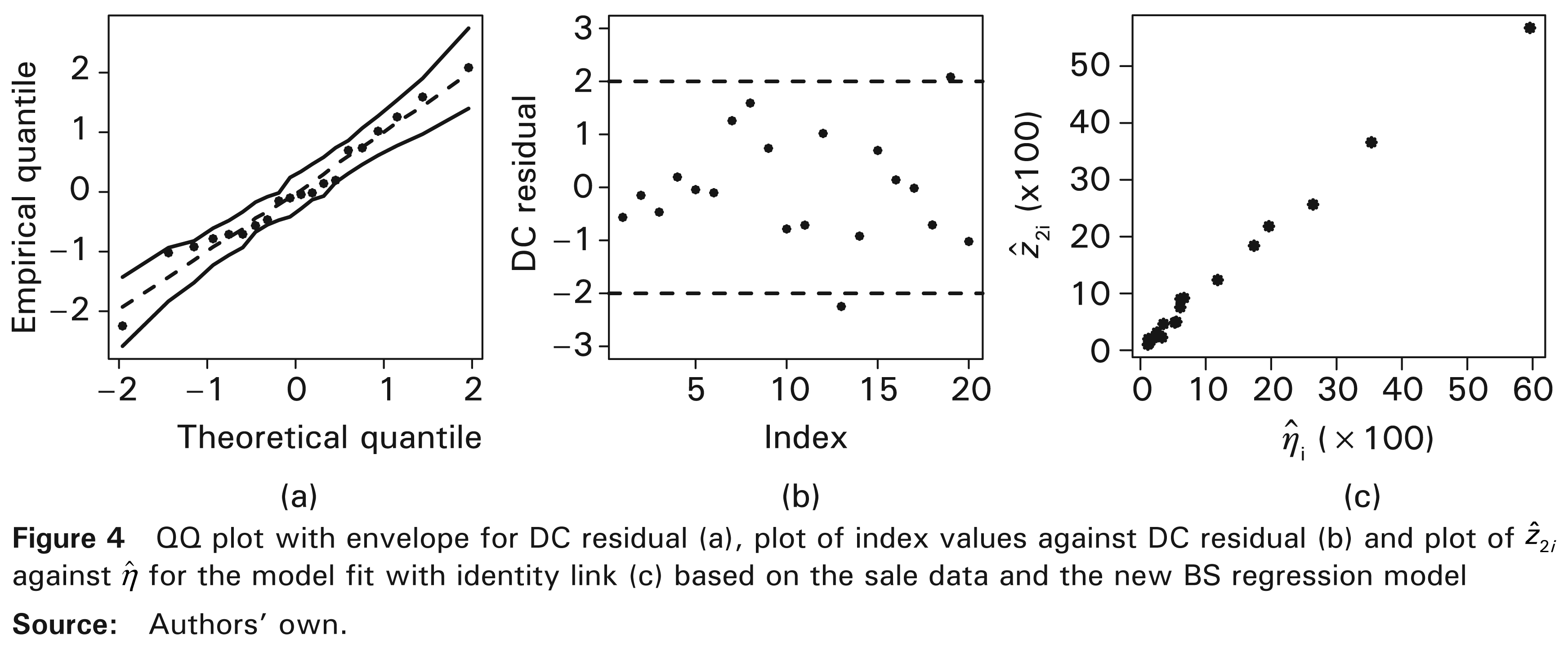
The assumptions of the model given in (8.2) are verified by a residual analysis based on sale data. The normal probability plot with envelope for the DC residual (r(4)) provided in Figure 4(a) is used to verify the distributional assumption of the model given in (8.2). This figure does not show unusual features, so that the assumption that the response variable follows a BS distribution does not seem to be unsuitable. In addition, the independence assumption also is verified by the normal probability with envelope and by the plot of residuals displayed in Figure 4(b), from which outlying observations are not detected. In Section 3, we mentioned that one of the assumptions of the proposed model is that the relation between the variance and mean is described by
We also verify whether the identity link function used in the model given in (8.2) is correct or not. We have that
8.3 Diagnostic analysis
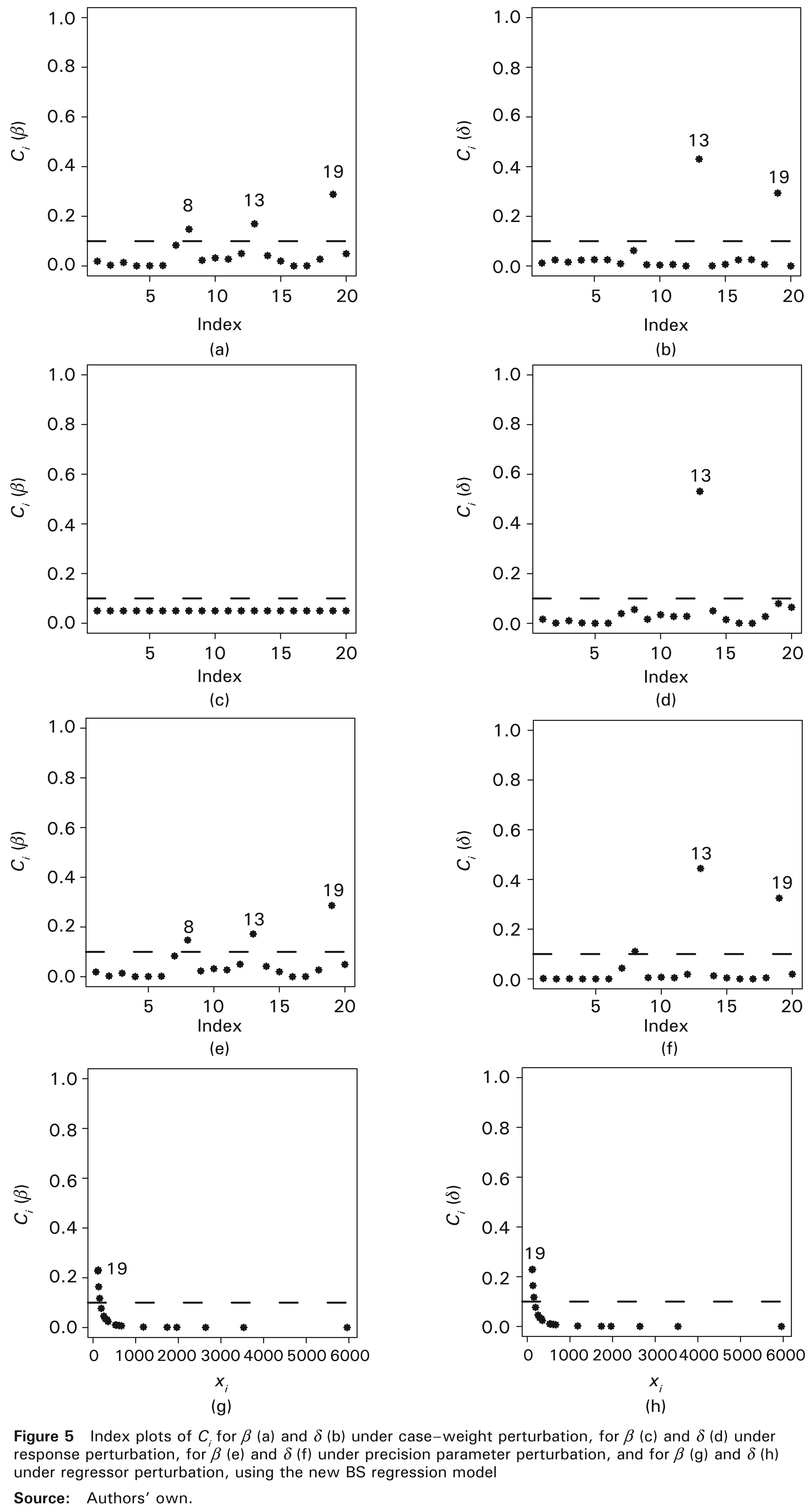
Influence diagnostics for the BS regression model given in (3.1) are presented in Figure 5. We also construct a GL plot (omitted here) based on the results of Section 5, which shows that observation #13 is a leverage point. Figure 5 displays index plots of Ci, from where observations #13 and #19 are detected as potentially influential. Also, we analyze index plots of |
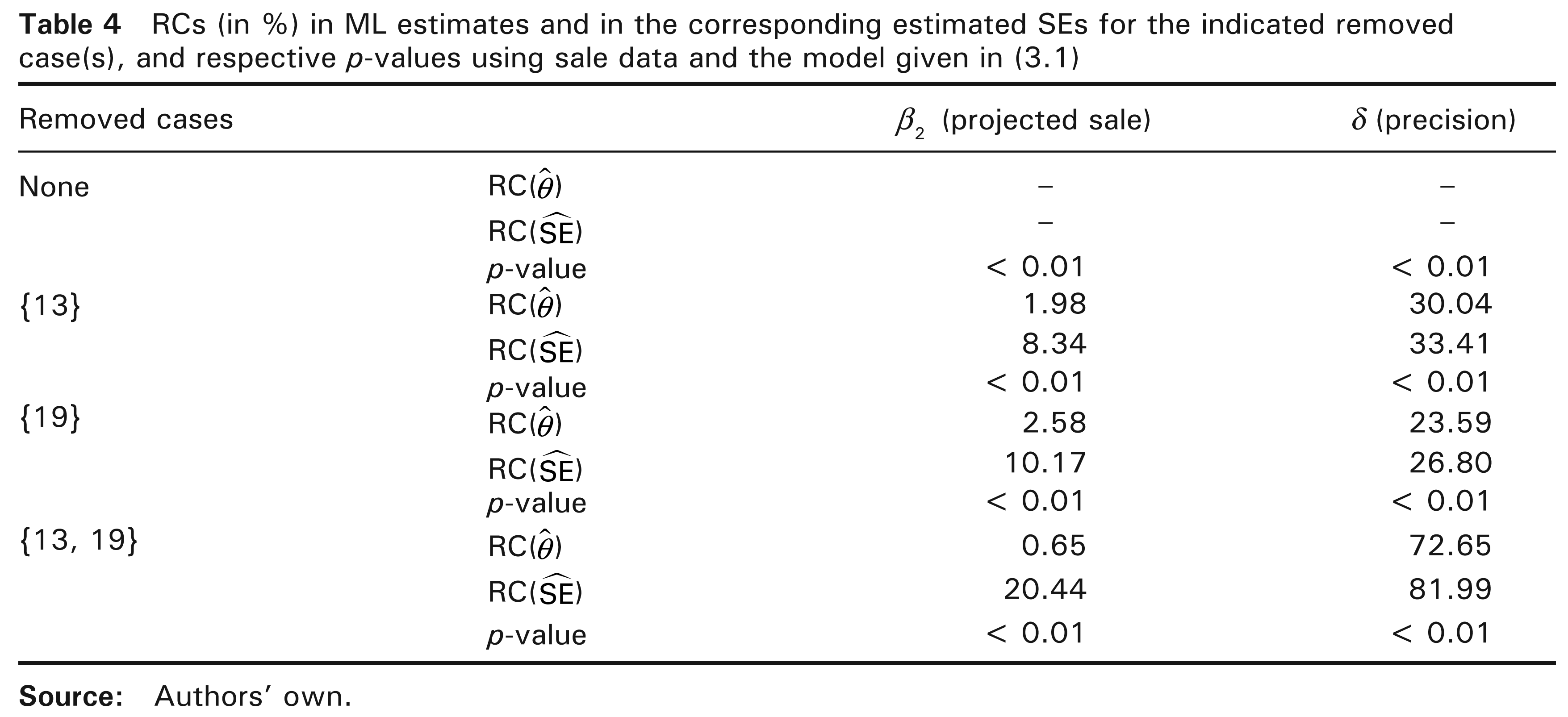
We now investigate the impact on the model inference when the cases detected as potentially influential in the diagnostic analysis are removed. Then, we again estimate the model parameters after removing the sets of observations {13}, {19} and {13, 19}. Table 4 provides the relative changes (RCs) in the parameter estimates and in their corresponding estimated SEs, by using the sale data. These changes are calculated from

where
8.4 The sale prediction model
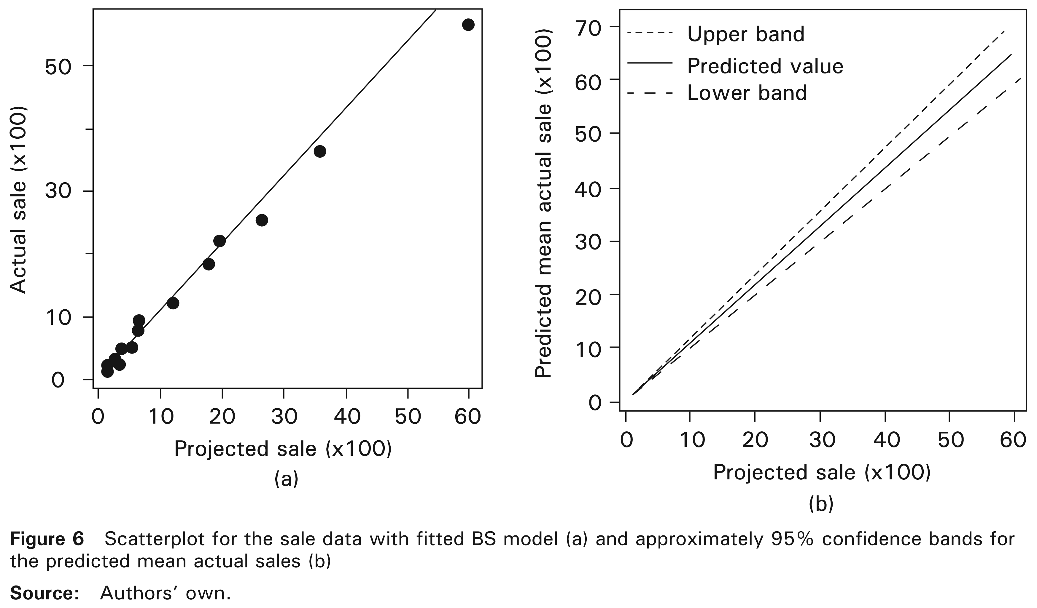
Figure 6(a) shows a scatterplot of projected sales against actual sales, with the estimated model given in (8.2). Note that the fitted line (proposed model) has a good agreement with the real data. We may interpret the estimated coefficients of the final model given in (8.3) as follows. Suppose that the projected sale value increases by p × 100%, so that the projected value is given by xp = [1 + p]x, for 0 < p < 1. Thus, the predicted mean sale value is given by µ(xp) = β2[1 + p]x, and the mean ratio is

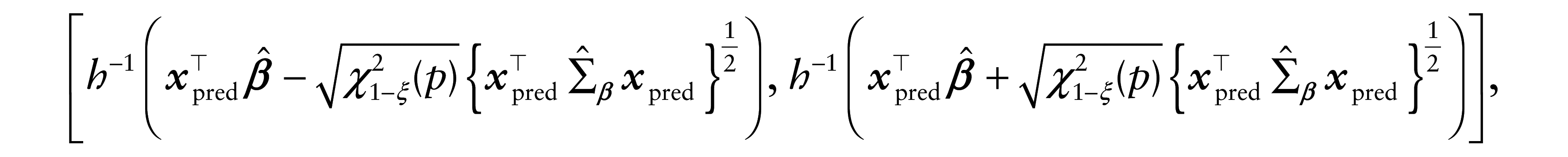
Therefore, if the projected sale increases p%, then the mean sale increases p% too. Based on (3.6) and considering the linear predictor µ(
RCs (in %) in ML estimates and in the corresponding estimated SEs for the indicated removed case(s), and respective p-values using sale data and the model given in (3.1)
9 Conclusions
The new BS regression models proposed in this article have characteristics that are unavailable in the models of this type existing in the literature. Specifically, the new models allow us to describe the mean of the data in their original scale, unlike the existing models, which employ a logarithmic transformation of the data, provoking a possible reduction of the power of the study and difficulties of interpretation. In addition, the new models enable us to describe data with non-constant variance. None of the existing BS models can simultaneously describe all these aspects. Furthermore, the new models are very flexible, because they permit us to use different non-negative link functions to relate the mean with the regressors. We have proposed four types of residuals for the new models and conducted a simulation study to establish their empirical properties in order to evaluate their performances. From this study, we have detected that the deviance component residual, usually employed in generalized linear models, is the most appropriate, which is coherent because the new models have been proposed using a similar idea to these generalized linear models. Moreover, we have developed methods of local influence to assess the potential influence of some observations on the model by using several perturbation schemes. Finally, we have performed a statistical modelling with real data by using the new approach proposed in the article, which have shown the importance of our proposal. The methodology introduced in this article has been implemented in the R software and it is available to interested users.
Footnotes
Acknowledgements
The authors thank the Editor, Professor Jeffrey Simonoff, an anonymous Associate Editor and two anonymous referees for their constructive comments on an earlier version of this manuscript, which resulted in this improved version. The authors gratefully acknowledge financial support from CAPES, CNPq and FACEPE, Brazil, and from FONDECYT 1120879 grant, Chile.
Hessian matrix
For the BS regression model given in (3.1), the second derivative of to βj and βi, for j, l = 1, …, p, is
we can group the values obtained in matrix form as
where to βj and δ, for j = 1, …, p, is
where ai is the ith element of to δ is
the expression given in (A3) can be represented in matrix form as
Then, the Hessian matrix can be expressed as