A model for overdispersed hierarchical ordinal data

Abstract

Non-Gaussian outcomes are frequently modelled using members of the exponential family. In particular, the Bernoulli model for binary data and the Poisson model for count data are well-known. Two reasons for extending this family are (1) the occurrence of overdispersion, implying that the variability in the data is not adequately described by the models, and (2) the incorporation of hierarchical structure in the data. These issues are routinely addressed separately, the first one through overdispersion models, the second one, for example, by means of random effects within the generalized linear mixed models framework. Molenberghs et al. (2007, 2010) introduced a so-called ‘combined model’ that simultaneously addresses both. In these and subsequent papers, a lot of attention was given to binary outcomes, counts, and time-to-event responses. While common in practice, ordinal data have not been studied from this angle. In this article, a model for ordinal repeated measures, subject to overdispersion, is formulated. It can be fitted without difficulty using standard statistical software. The model is exemplified using data from an epidemiological study in diabetic patients and using data from a clinical trial in psychiatric patients.

Keywords

beta distribution generalized linear mixed model maximum likelihood proportional odds model overdispersion

1 Introduction

Next to continuous and binary outcomes, count data features are extensively covered in the modelling literature and play a prominent role in applied statistical work. It is common to place such models in a generalized linear modelling (GLM) framework (Nelder and Wedderburn, 1972; McCullagh and Nelder, 1989; Agresti, 2002). It allows one to specify either the first and second moments only or the full distribution. In the latter case, the exponential family (McCullagh and Nelder, 1989) has been of particular interest, given that it provides an elegant and encompassing mathematical framework with the normal, Bernoulli/binomial, and Poisson models as prominent members.

The elegance of the GLM framework draws from certain linearity properties of the log-likelihood function, leading to mathematically convenient score equations and ultimately to a straightforward use of inferential instruments, both in terms of estimation and inference. A key feature of the GLM model and the exponential family is the ‘mean-variance relationship’, a term used to indicate that the variance v is a deterministic function of the mean . For example, for Bernoulli outcomes with success probability , the variance is $v () (1)$ , while for counts following the Poisson model, the relationship is even simpler, i.e., $v ()$ . In contrast, the mean and variance are entirely separate parameters in case of continuous normally distributed outcomes. Finally, while independently and identically distributed (i.i.d.) binary data cannot contradict the mean-variance relationship, i.i.d. counts can.

The above explains why most early work was on formulating models that explicitly allow for a dispersion not following the base models. It is often referred to as overdispersion, but underdispersion can occur as well. Hinde and Demétrio (1998a, 1998b) provide broad overviews of approaches for dealing with overdispersion, considering moment-based as well as full-distribution avenues. For purely binary data, the mean-variance link can only be violated in case of hierarchical data, e.g., in case of longitudinal data, where an outcome is recorded repeatedly over time for a number of study subjects. Apart from overdispersion, hierarchies in the data imply associations between measurements on the same unit as well. Thus, a flexible parametric model ought to properly capture the mean function, the variance function, and the association function. The so-called generalized linear mixed model (GLMM; Breslow and Clayton, 1993; Wolfinger and O’Connell, 1993; Engel and Keen, 1994; Molenberghs and Verbeke, 2005) has become the dominant tool for hierarchical non-Gaussian data.

Molenberghs, Verbeke and Demétrio (2007; henceforth MVD) and Molenberghs, Verbeke, Demétrio and Vieira (2010; henceforth MVDV) and Molenberghs, Verbeke, Iddi and Demétrio (2012; henceforth MVID) showed that accommodating either overdispersion or hierarchically-induced association may fall short when properly modelling the data. MVD focused on counts, MVDV laid out a general framework, whereas MVID tackles binary and binomial outcomes. The topic of the current article is the modelling of repeated, overdispersed ordinal data.

The article is structured out as follows. In Section 2, two motivating case studies are introduced; they are analyzed in Section 6. It will be shown that the first one shows strong overdispersion and correlation, while the second study will enable to study the model’s behaviour when in fact overdispersion is absent. Section 3 briefly summarizes relevant modelling background; the proposed model for repeated, overdispersed ordinal outcomes is presented in Section 4. Parameter estimation is considered in Section 5.

2 Motivating case studies

2.1 Fluvoxamine trial

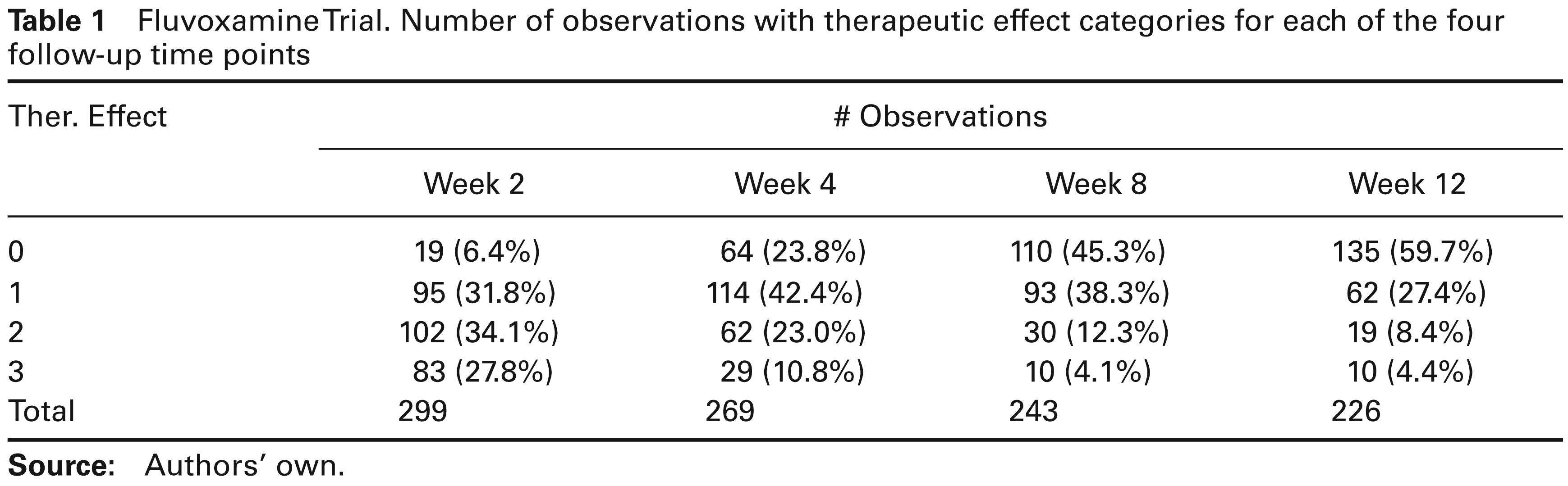
This study is concerned with psychiatric symptoms allegedly resulting from a dysregulation of serotonine in the brain. A multicentre study was undertaken, enrolling 315 patients that were treated by fluvoxamine. The data are discussed in several places, including Molenberghs and Verbeke (2005), Molenberghs and Lesaffre (1994), Kenward, Lesaffre, and Molenberghs (1994), Molenberghs, Kenward, and Lesaffre (1997), and Michiels and Molenberghs (1997). Once recruited, patients were assessed at four visits. The therapeutic effect and the extent of side effects were scored at each visit on an ordinal scale. The side effect response is coded as (1) none; (2) not interfering with functionality; (3) interfering significantly with functionality; (4) side effects surpasses the therapeutic effect. Similarly, the effect of therapy is recorded on a four-point ordinal scale: (1) no improvement or worsening; (2) minimal improvement; (3) moderate improvement and (4) important improvement. Thus, a side effect occurs if new symptoms occur while there is therapeutic effect if old symptoms disappear. A total of 299 patients have at least one measurement, including 242 completers. There is also baseline covariate information on each subject, including gender, age, presence of psychiatric antecedents, initial severity of the disease, duration of the actual mental illness. A summary is given in Table 1.

Table 1
Fluvoxamine Trial. Number of observations with therapeutic effect categories for each of the four follow-up time points

Ther. Effect # Observations

Week 2 Week 4 Week 8 Week 12

0 19 (6.4%) 64 (23.8%) 110 (45.3%) 135 (59.7%)

1 95 (31.8%) 114 (42.4%) 93 (38.3%) 62 (27.4%)

2 102 (34.1%) 62 (23.0%) 30 (12.3%) 19 (8.4%)

3 83 (27.8%) 29 (10.8%) 10 (4.1%) 10 (4.4%)

Total 299 269 243 226

Ther. Effect	# Observations
0	19 (6.4%)	64 (23.8%)	110 (45.3%)	135 (59.7%)
1	95 (31.8%)	114 (42.4%)	93 (38.3%)	62 (27.4%)
2	102 (34.1%)	62 (23.0%)	30 (12.3%)	19 (8.4%)
3	83 (27.8%)	29 (10.8%)	10 (4.1%)	10 (4.4%)
Total	299	269	243	226

Source: Authors’ own.

2.2 Diabetes study

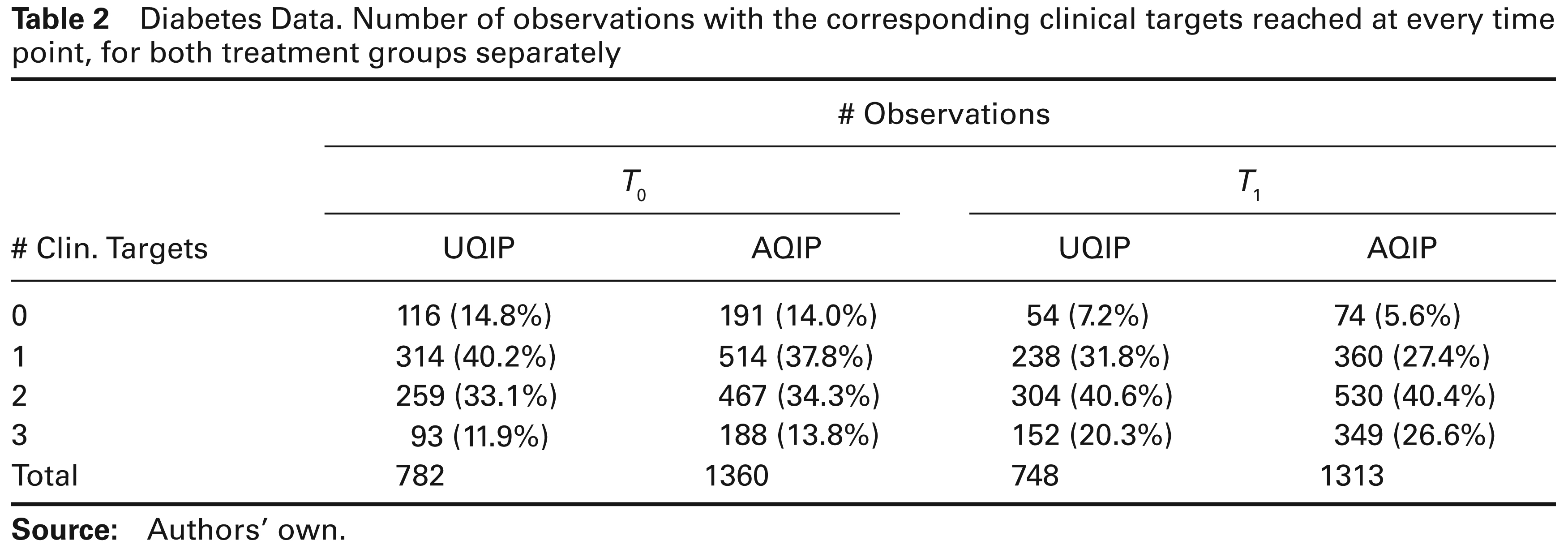
In Belgium, the diabetes project was conducted from January 2005 until December 2006, with the aim to study the effect of implementing a structured model for chronic diabetes care on the patients’ clinical outcomes. General practitioners (GPs) were offered assistance and could redirect patients to the diabetes care team, consisting of a nurse educator, a dietician, an ophthalmologist, and an internal medicine doctor. For the project, two programmes were implemented and GPs were randomized to one of two groups: UQIP: Usual Quality Improvement Programme and AQIP: Advanced Quality Improvement Programme. A total of 120 GPs took part in the study, 53 in the UQIP group and 67 in the AQIP group, including 918 and 1577 patients, respectively.

Table 2
Diabetes Data. Number of observations with the corresponding clinical targets reached at every time point, for both treatment groups separately

# Clin. Targets # Observations

T₀
T₁

UQIP AQIP UQIP AQIP

0 116 (14.8%) 191 (14.0%) 54 (7.2%) 74 (5.6%)

1 314 (40.2%) 514 (37.8%) 238 (31.8%) 360 (27.4%)

2 259 (33.1%) 467 (34.3%) 304 (40.6%) 530 (40.4%)

3 93 (11.9%) 188 (13.8%) 152 (20.3%) 349 (26.6%)

Total 782 1360 748 1313

# Clin. Targets	# Observations
0	116 (14.8%)	191 (14.0%)	54 (7.2%)	74 (5.6%)
1	314 (40.2%)	514 (37.8%)	238 (31.8%)	360 (27.4%)
2	259 (33.1%)	467 (34.3%)	304 (40.6%)	530 (40.4%)
3	93 (11.9%)	188 (13.8%)	152 (20.3%)	349 (26.6%)
Total	782	1360	748	1313

Source: Authors’ own.

During the project, several outcomes useful to evaluate how well diabetes is controlled were measured, at the moment the programme was initiated (time T₀) and one year later (T₁). The most important outcomes were HbA1c (glycosylated hemoglobin), LDL-cholesterol (low-density lipoprotein cholesterol) and SBD (systolic blood pressure). Furthermore, experts specified cut off values defining so-called ‘a clinical target’ for each outcome: HBA1C < 7%, LDL-cholesterol < 100 mg/dl and SBD # 130 mmHg. As a result, for a particular time point, every patient could reach minimum 0–maximum 3 clinical targets. This number was reflected in the variable ‘number of clinical targets’. If at least one measurement per patient was missing, the value for the number of clinical targets was set to missing as well. The data are discussed in Borgermans et al. (2009). A summary is given in Table 2.

3 Background on the exponential family

A fundamental tool, in general and for us here, is the exponential family (Jørgensen, 1987; McCullagh and Nelder, 1989). The generic density for a random variable Y is then:

f (y) f (y |,) \exp \{^{1} [y ()] c (y,)\},

(3.1)

where is the natural parameter and the dispersion parameter; $()$ is the generating function and $c (,)$ is the normalizing function. The mean is $E (Y)^{} ()$ , and the variance equals:

Var (Y)^{2} {^{}}^{} ().

(3.2)

The model naturally leads to a so-called mean–variance relationship: $^{2}^{} [{^{}}^{1} ()] v ()$ , with v(.) the variance function.

The mean , through the function , can depend on covariates x_i for outcome Y_i, with i = 1, …, N. Precisely, $_{i} h (_{i}) h ({x_{i}}^{})$ , for a known function h(.), the inverse link function. The model is termed ‘GLM’. The link function $h ()^{} ()$ is called the natural link, in which case $_{i} {x_{i}}^{}$ . Popular routes for parameter estimation include maximum likelihood and quasi likelihood.

The mean–variance relation can be restrictive. The phenomenon where the empirical variance does not obey the prescribed mean–variance relationship is termed overdispersion. Hinde and Demétrio (1998a, 1998b) offer reviews as to how the GLM can be modified to accommodate overdispersion. One route is via the overdispersion parameter $1$ , so that (3.2) leads to $Var (Y) v ()$ . A route taken up further in this article is the accommodation of overdispersion via random effects. One then combines a model $f (y_{i} |_{i})$ for the outcome given a random effect $_{i}$ with a model for the random effect itself, $f (_{i})$ say. The implied marginal model for Y_i then follows by integration:

f (y_{i}) f (y_{i} |_{i}) f (_{i}) d_{i} .

(3.3)

Two natural ways to introduce random effects into the GLM framework are either by the use of a so-called conjugate distribution (in the sense of Cox and Hinkley, 1974, p. 370, and Lee, Nelder and Pawitan, 2006, p. 178) for the parameter or by including normal random effects into the linear predictor. Mathematically,

f (y |) \exp \{^{1} [yh () g ()] c (y,)\},

(3.4)

f () \exp \{[h () g ()] c * (,)\},

(3.5)

where $g ()$ and $h ()$ are functions, , , and are parameters, and also here normalizing functions, $c (y,)$ and $c * (,)$ , are used to ensure that (3.4)–(3.5) are proper densities. The ensuing marginal model is:

f (y) \exp [c (y,) c * (,) c * (^{1}, \frac{^{1} y}{^{1}})] .

(3.6)

When Y_i would be Bernoulli, then conjugacy leads to the beta distribution for $_{i}$ . By analogy, we will also here opt for the beta distribution, although its use with ordinal data is less straightforward than in the dichotomous case. The rationale is that ordinal outcomes with R categories are conveniently represented by R – 1 non-redundant dummies, so that the beta distribution remains to be an obvious choice.

For longitudinal or otherwise hierarchical data, the GLMM (Breslow and Clayton, 1993; Wolfinger and O’Connell, 1993; Engel and Keen, 1994) is popular. Let now Y_ij be outcome j = 1, …, n_i for subject i = 1, …, N, and let Y _i be the vector consisting of the Y_ij. Assume that, conditionally upon q-dimensional random effects b_i + N(0, D), the outcomes Y_ij are independent with densities:

f_{i} (y_{ij} | b_{i},,) \exp \{^{1} [y_{ij}_{ij} (_{ij})] c (y_{ij},)\},

(3.7)

where

[^{} (_{ij})] (_{ij}) [E (Y_{ij} | b_{i},)] {x^{}}_{ij} {z^{}}_{ij} b_{i}

(3.8)

for a given link function $()$ , with x _ij and z _ij p-dimensional and q-dimensional vectors of known covariate values, and also with a p-dimensional vector of unknown fixed regression coefficients. Further, is a scale or overdispersion parameter. To complete the specification, let $f (b_{i} | D)$ be the density of the N(0, D) distribution for the random effects b_i. MVID indicated that D models both correlation among repeated measures and overdispersion. Relying on a single set of parameters for these two tasks is often too restrictive, motivating the extension of the next section.

4 A Combined proportional Odds-Beta-Normal model

Assume the ordinal outcome Y_ij can take values r = 1, …, R. We replace it by a set of R dummies:

Z_{r, ij} \{\begin{matrix} 1 & if Y_{r, ij} r, \\ 0 & otherwise, \end{matrix}

for r = 1, …, R. Evidently, there are redundant dummies, but any subset of R – 1 components is not. Group the dummies into vectors Z _ij and Z _i for a specific subject i and occasion j, and for a specific subject i, respectively. We assume a multinomial distribution $Z_{ij} multinomial (_{ij})$ , with $_{ij} (_{1, ij},,_{r, ij},,_{R, ij})$ . The multinomial distribution at a given occasion is determined by the modelling choice for the ordinal outcome. Under a proportional odds assumption, using normal random effects b _i + N(0, D) in the linear predictor, and beta random effects $_{ij} Beta (_{j},_{j})$ to capture further overdispersion, the probabilities can be written as:

_{r, ij} \{\begin{matrix} _{ij}_{1, ij} & if r 1, \\ _{ij} (_{r, ij}_{r 1, ij}) & if 1 < r < R, \\ 1_{ij}_{R 1, ij} & if r R . \end{matrix}

(4.1)

where

_{r, ij} \frac{\exp (_{0 r} {x^{}}_{ij} {z^{}}_{ij} b_{i})}{1 \exp (_{0 r} {x^{}}_{ij} {z^{}}_{ij} b_{i})} .

(4.2)

Here, $_{01}_{0, R 1}$ are intercepts, are fixed regression coefficients, and x_ij ( z_ij ) is the design vector for the fixed (random) effects at occasion j. Some choices in the above can be relaxed and/or altered. For example, the $_{j}$ and $_{j}$ parameters, describing the beta distribution, need not be dependent on j. To ensure identifiability, a constraint needs to be applied to it, e.g., $_{j}_{j} 1$ , but it is mathematically convenient to retain them as two separate parameters, with the understanding that the constraint does apply. Finally, the $_{ij}$ within a subject are assumed different from each other and independent. One could allow them to be correlated, or even constant across subjects. This will not be considered here.

As argued in MVDV and MVID, closed-form expressions for marginal means, variances, covariances, and even the entire marginal distribution, i.e., integrated over both sets of random effects, cannot be derived in the binary case with logit link and normal random effects (regardless of the overdispersion random effects). Evidently, the same will be true for the ordinal case. If necessary, numerical integration or other Monte Carlo methods can be used to derive such marginal quantities.

5 Parameter estimation

MVID mentioned several possible estimation strategies, then focused on maximum likelihood. Because likelihood inference is based on the marginal density of the outcomes, one needs to integrate over the normal and beta random effects. MVID proceeded by analytically integrating over the beta random effects, leading to a so-called partially marginalized density. In our case, this takes the form:

f (y_{ij} | b_{i}) \frac{_{j}}{_{j}_{j}} (_{1, ij})^{z_{1, ij}}_{r 2}^{R 1} (_{r, ij}_{r 1, ij})^{z_{r, ij}} {(\frac{_{j}_{j}}{_{j}}_{R 1, ij})}^{z_{R, ij}} .

Then, a generic maximum likelihood routine that allows for integration over normal random effects can be used. We follow this route and use the SAS procedure NLMIXED to this effect. The following choices were made for conducting integration: adaptive Gaussian quadrature, which is more accurate than ordinary Gaussian quadrature (Molenberghs and Verbeke, 2005); the number Q of quadrature points is preferably user-defined than selected in an automated way and, once converged, a numerical sensitivity analysis to check whether Q was chosen sufficiently large is advisable.

6 Data analysis

6.1 Fluvoxamine trial

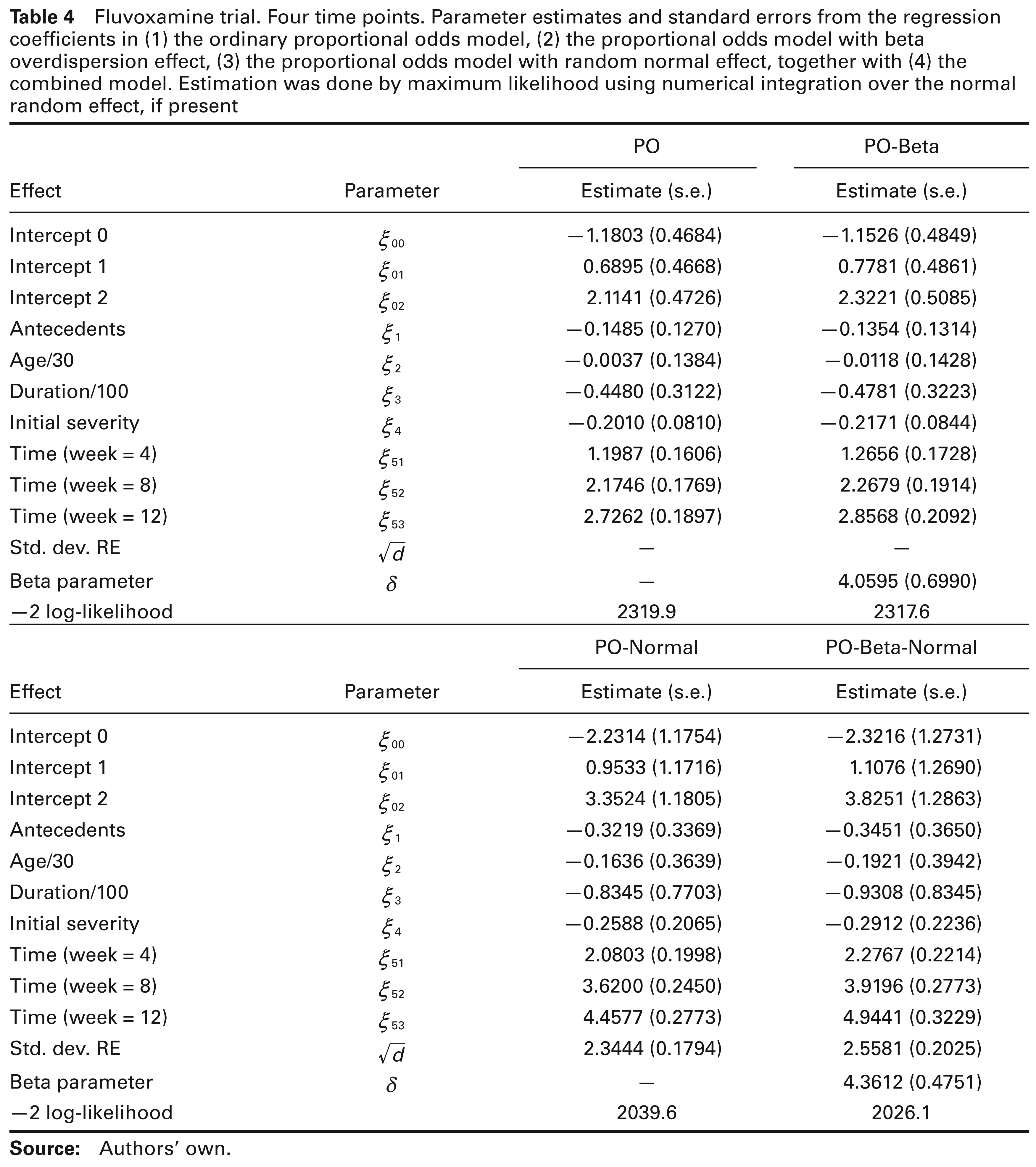
The fluvoxamine trial encompasses four time points. The response studied here is the therapeutic effect, rated on a four-point ordinal scale, as explained in Section 2.1. Two versions are analyzed. First, we use the measurements from the first and the last clinical visits only (week 2 and week 12). Second, all four measurements (weeks 2, 4, 8, and 12) are used. Juxtaposing both can be seen as an informal sensitivity analysis, investigating numerical stability, identifiability, etc. Also, the two-time-point case is similar to the diabetes data set, analyzed in the previous section. The results are presented in Tables 3 and 4. Covariate effects were retained by way of backward selection. Covariates considered are psychiatric antecedents (X_2i), age (X_3i), duration of the illness (X_4i), and initial severity (X_5i). In the analysis of all four repeated measurements, time was allowed to have a differential effect at the various time points.

Let Y_ij be the score of the therapeutic effect for patient i at time point j. We consider the same set of four models as for the diabetes study. The combined proportional odds logistic model for the two-time-point case equals:

\log it [P (Y_{ij} r | t_{ij}, X_{1 i},, X_{4 i})]_{0 r} b_{i}_{1} X_{1 i}_{4} X_{4 i}_{5} t_{ij},

(r = 0, …, 3). For the four-times case the model takes the form:

\log it [P (Y_{ij} r | t_{1 ij}, t_{2 ij}, t_{3 ij}, X_{1 i},, X_{4 i})]

_{0 r} b_{i}_{1} X_{1 i}_{4} X_{4 i}_{51} t_{1 ij}_{52} t_{2 ij}_{53} t_{3 ij},

where t_1ij, t_2ij and t_3ij are dummies corresponding to weeks 4, 8, and 12.

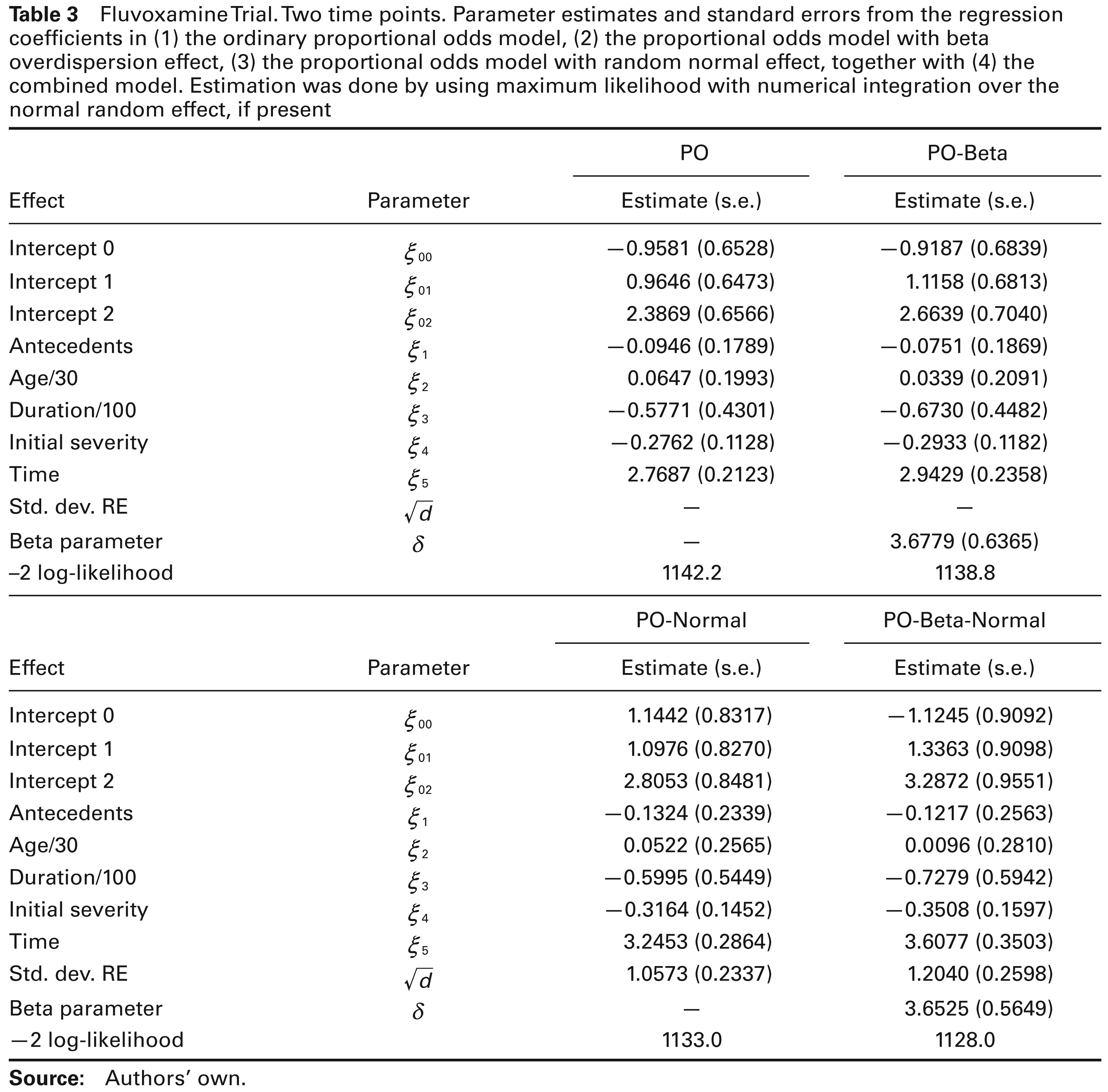
The results obtained here differ qualitatively from the ones reached for the diabetes study. There clearly is an improvement in terms of the likelihood when moving to the overdispersion models, already for the case of only two time points. We will study these model comparisons more formally, realizing that there are some subtle issues.

Table 3
Fluvoxamine Trial. Two time points. Parameter estimates and standard errors from the regression coefficients in (1) the ordinary proportional odds model, (2) the proportional odds model with beta overdispersion effect, (3) the proportional odds model with random normal effect, together with (4) the combined model. Estimation was done by using maximum likelihood with numerical integration over the normal random effect, if present

Effect Parameter PO
PO-Beta

Estimate (s.e.) Estimate (s.e.)

Intercept 0 $_{00}$ —0.9581 (0.6528) —0.9187 (0.6839)

Intercept 1 $_{01}$ 0.9646 (0.6473) 1.1158 (0.6813)

Intercept 2 $_{02}$ 2.3869 (0.6566) 2.6639 (0.7040)

Antecedents $_{1}$ —0.0946 (0.1789) —0.0751 (0.1869)

Age/30 $_{2}$ 0.0647 (0.1993) 0.0339 (0.2091)

Duration/100 $_{3}$ —0.5771 (0.4301) —0.6730 (0.4482)

Initial severity $_{4}$ —0.2762 (0.1128) —0.2933 (0.1182)

Time $_{5}$ 2.7687 (0.2123) 2.9429 (0.2358)

Std. dev. RE $\sqrt{d}$ — —

Beta parameter — 3.6779 (0.6365)

–2 log-likelihood

1142.2
1138.8

Effect
Parameter
PO-Normal
PO-Beta-Normal

Estimate (s.e.)
Estimate (s.e.)

Intercept 0 $_{00}$ 1.1442 (0.8317) —1.1245 (0.9092)

Intercept 1 $_{01}$ 1.0976 (0.8270) 1.3363 (0.9098)

Intercept 2 $_{02}$ 2.8053 (0.8481) 3.2872 (0.9551)

Antecedents $_{1}$ —0.1324 (0.2339) —0.1217 (0.2563)

Age/30 $_{2}$ 0.0522 (0.2565) 0.0096 (0.2810)

Duration/100 $_{3}$ —0.5995 (0.5449) —0.7279 (0.5942)

Initial severity $_{4}$ —0.3164 (0.1452) —0.3508 (0.1597)

Time $_{5}$ 3.2453 (0.2864) 3.6077 (0.3503)

Std. dev. RE $\sqrt{d}$ 1.0573 (0.2337) 1.2040 (0.2598)

Beta parameter — 3.6525 (0.5649)

—2 log-likelihood 1133.0 1128.0

Effect	Parameter	PO	PO-Beta
Intercept 0	$_{00}$	—0.9581 (0.6528)	—0.9187 (0.6839)
Intercept 1	$_{01}$	0.9646 (0.6473)	1.1158 (0.6813)
Intercept 2	$_{02}$	2.3869 (0.6566)	2.6639 (0.7040)
Antecedents	$_{1}$	—0.0946 (0.1789)	—0.0751 (0.1869)
Age/30	$_{2}$	0.0647 (0.1993)	0.0339 (0.2091)
Duration/100	$_{3}$	—0.5771 (0.4301)	—0.6730 (0.4482)
Initial severity	$_{4}$	—0.2762 (0.1128)	—0.2933 (0.1182)
Time	$_{5}$	2.7687 (0.2123)	2.9429 (0.2358)
Std. dev. RE	$\sqrt{d}$	—	—
Beta parameter		—	3.6779 (0.6365)
–2 log-likelihood		1142.2	1138.8
Effect	Parameter	PO-Normal	PO-Beta-Normal
Estimate (s.e.)	Estimate (s.e.)
Intercept 0	$_{00}$	1.1442 (0.8317)	—1.1245 (0.9092)
Intercept 1	$_{01}$	1.0976 (0.8270)	1.3363 (0.9098)
Intercept 2	$_{02}$	2.8053 (0.8481)	3.2872 (0.9551)
Antecedents	$_{1}$	—0.1324 (0.2339)	—0.1217 (0.2563)
Age/30	$_{2}$	0.0522 (0.2565)	0.0096 (0.2810)
Duration/100	$_{3}$	—0.5995 (0.5449)	—0.7279 (0.5942)
Initial severity	$_{4}$	—0.3164 (0.1452)	—0.3508 (0.1597)
Time	$_{5}$	3.2453 (0.2864)	3.6077 (0.3503)
Std. dev. RE	$\sqrt{d}$	1.0573 (0.2337)	1.2040 (0.2598)
Beta parameter		—	3.6525 (0.5649)
—2 log-likelihood		1133.0	1128.0

Source: Authors’ own.

To compare the PO and PO-Beta models for the case of two time points, the likelihood ratio test can be used. The difference in deviance is 3.4. However, care has to be taken when comparing such models, because of the special status of variance components. As explained in Verbeke and Molenberghs (2000), and further expanded upon in Verbeke and Molenberghs (2003) and Molenberghs and Verbeke (2007), two views can be taken. In a hierarchical view, the variance components are formally considered to describe random effects, and hence have the meaning of a variance (like d) or a variance parameter (like ). As a consequence, the null value lies on the boundary of the parameter space, turning this into a non-standard situation. Based upon the work by Stram and Lee (1994, 1995), Self and Liang (1987), Verbeke and Molenberghs (2003) and Molenberghs and Verbeke (2007), the likelihood ratio, score, and Wald tests then do not follow the conventional asymptotic $^{2}$ null distributions, but rather take the form of mixtures of such $^{2}$ distributions. Precisely which one to apply depends on the geometry of the null space. For a single variance parameter, this is a 50:50 mixture of a $_{0}^{2}$ (the degenerate distribution in 0) and a $_{1}^{2}$ , often denoted as $_{0 : 1}^{2}$ . Comparing the PO and PO-Beta models, we obtain $p P (_{0 : 1}^{2} 3.4) 0.5 P (_{0}^{2} 3.4) 0.5 P (_{1}^{2} 3.4) 0.0326$ . In contrast, under a marginal view the only condition imposed on the model is that the marginal distribution be valid. This is a weaker condition, as now the ranges of the variance parameters expand. Importantly, the null value then no longer lies on the boundary of the parameter space, and the problem is regular again. In fact, the variance parameters should now merely be viewed as variance components. In the beta-binomial model, to which the PO-Beta model is very strongly linked, the interpretation is that marginally, the model can produce negative intra-cluster correlation, whereas the marginal model is restricted to non-negative association. In this case, a comparison between PO and PO-Beta produces: $p P (_{1}^{2} 3.4) 0.0652$ . Evidently, this p-value simply is double its hierarchical counterpart, which follows from the nature of this specific mixture. Clearly, the choice matters, because in this case we land at different sides of the 0.05 cut-off value. For the situation of four time points, the likelihood ratio test statistic is 2.3 with p-values of 0.0647 and 0.1294, under the hierarchical and marginal views, respectively.

Likewise, when comparing the PO-Normal and PO-Beta-Normal models, the same null distributions apply. The likelihood ratio test statistic now takes the value 5. The hierarchical p-value, again from a $_{0 : 1}^{2}$ , is 0.0127, with its marginal counterpart being 0.0253. The test statistic with four time points is 13.5, and $p < 0.0001$ and $p 0.0002$ , respectively. Further, we can compare the PO with the PO-Normal, which is a classical test for the need of the random-intercepts variance $d$ . The same mixture distribution should be used here as well. Hierarchically, we find $p 0.0012$ , whereas the marginal counterpart is $p 0.0024$ . Comparing PO-Beta and PO-Beta-Normal produces, hierarchically, $p 0.0005$ and marginally $p 0.0010$ . In the four-time-points case, the corresponding likelihood ratio test statistics are all very large, and all $p < 0.0001$ .

Finally, we can compare PO and PO-Beta-Normal directly. This situation is different from all previous ones, because we now test for two variance components at the same time. Both lie on the boundary of the parameter space, and there is no covariance term between them. This ‘variance-component’ situation was discussed also by Verbeke and Molenberghs (2003). The likelihood ratio test statistic in the two-time-points case is 14.2, with hierarchical $p 0.25 P (_{0}^{2} 14.2) 0.5 P$ $(_{1}^{2} 14.2) 0.25 P (_{2}^{2} 14.2) 0.0003$ . The marginal counterpart is $p P (_{2}^{2}$ $14.2) 0.0008$ . Note that, this time, the marginal p-value is not merely twice the hierarchical version.

From this analysis, we also deduce that there is weak or no evidence for the need of a beta random effect when comparing PO and PO-Beta with two time points. However, the corresponding assessment based on comparing the PO-Normal model and the PO-Beta-Normal model provides much stronger evidence for the need for such beta random effects. In other words, while there seems little evidence for overdispersion based on the model without normal random effects, the need for overdispersion becomes evident when the random effects in the data are accounted for. This strongly suggests that the incorporation of one of the sources of variability may not tell the entire story. We therefore recommend starting model building from the most general model, the PO-Beta-Normal in this case, and then examining whether simplification is possible.

Which model is chosen also has an impact on resulting inference. Consider the time effect based on the model with two time points. The corresponding z-ratio takes values 13.04, 12.48, 11.33, and 10.30 for the PO, PO-Beta, PO-Normal and PO-Beta-Normal models, respectively. Even though not spectacular, the impact is noticeable. Equally, the impact on resulting confidence intervals should not be discarded.

6.2 Diabetes study

We will analyze the diabetes data, introduced in Section 2.2. The rationale for this case study is to contrast it with the previous study. Indeed, the fluvoxamine study exhibits strong correlation and overdispersion, whereas there will be little or no overdispersion here. Because in such a case the beta parameter is expected to grow large, the model could be relatively unstable to fit and therefore empirical evidence needs to be built as to the model’s performance. The issue is known in particular for the combined model in the binary case (Molenberghs et al., 2012), reinforcing the fact that it needs to be scrutinized here too.

Let $Y_{ij} 0,, 3$ be the number of clinical targets patient i reached at time point j. Also, let $t_{ij} 0, 1$ be the time point at which the jth measurement was taken. Consider the combined proportional odds logistic regression model:

\log it [P (Y_{ij} r | t_{ij}, X_{i})]_{0 r} b_{i}_{1} t_{ij}_{2} X_{i},

$(r 0,, 3)$ , where the random intercept b_i is assumed $N (0, d)$ distributed, and $X_{i}$ is an indicator for group. The beta random effect is re-parameterized such that:

\frac{e^{}}{1 e^{}} \frac{}{},

thus simultaneously avoiding identifiability and range violation issues. The parameter is the one entered into the likelihood function. We consider (1) the ordinary proportional odds model, (2) the proportional odds model with beta overdispersion effect, (3) the proportional odds model with random normal effect, and (4) the combined model. Estimates (standard errors) are presented in Table 5. Clearly, there is no significant improvement, neither when we switch from model (1) to model (2), nor when we move from (3) to (4). The estimate for the beta-parameter is large and has a very large standard error. This indicates that there is no overdispersion in the data, in line also with what is observed for binary data (Molenberghs et al., 2012). Fortunately, even though the parameter in the PO-Beta and PO-Beta-Normal models grows large, as is expected because under complete absence of overdispersion , the models nicely converge and lead to reliable estimates and standard errors for the other model parameters. This is corroborated by comparing the left-hand and right-hand columns in Table 5.

Table 4
Fluvoxamine trial. Four time points. Parameter estimates and standard errors from the regression coefficients in (1) the ordinary proportional odds model, (2) the proportional odds model with beta overdispersion effect, (3) the proportional odds model with random normal effect, together with (4) the combined model. Estimation was done by maximum likelihood using numerical integration over the normal random effect, if present

Effect Parameter PO
PO-Beta

Estimate (s.e.) Estimate (s.e.)

Intercept 0 $_{00}$ —1.1803 (0.4684) —1.1526 (0.4849)

Intercept 1 $_{01}$ 0.6895 (0.4668) 0.7781 (0.4861)

Intercept 2 $_{02}$ 2.1141 (0.4726) 2.3221 (0.5085)

Antecedents $_{1}$ —0.1485 (0.1270) —0.1354 (0.1314)

Age/30 $_{2}$ —0.0037 (0.1384) —0.0118 (0.1428)

Duration/100 $_{3}$ —0.4480 (0.3122) —0.4781 (0.3223)

Initial severity $_{4}$ —0.2010 (0.0810) —0.2171 (0.0844)

Time (week = 4) $_{51}$ 1.1987 (0.1606) 1.2656 (0.1728)

Time (week = 8) $_{52}$ 2.1746 (0.1769) 2.2679 (0.1914)

Time (week = 12) $_{53}$ 2.7262 (0.1897) 2.8568 (0.2092)

Std. dev. RE $\sqrt{d}$ — —

Beta parameter — 4.0595 (0.6990)

—2 log-likelihood

2319.9
2317.6

Effect
Parameter
PO-Normal
PO-Beta-Normal

Estimate (s.e.)
Estimate (s.e.)

Intercept 0 $_{00}$ —2.2314 (1.1754) —2.3216 (1.2731)

Intercept 1 $_{01}$ 0.9533 (1.1716) 1.1076 (1.2690)

Intercept 2 $_{02}$ 3.3524 (1.1805) 3.8251 (1.2863)

Antecedents $_{1}$ —0.3219 (0.3369) —0.3451 (0.3650)

Age/30 $_{2}$ —0.1636 (0.3639) —0.1921 (0.3942)

Duration/100 $_{3}$ —0.8345 (0.7703) —0.9308 (0.8345)

Initial severity $_{4}$ —0.2588 (0.2065) —0.2912 (0.2236)

Time (week = 4) $_{51}$ 2.0803 (0.1998) 2.2767 (0.2214)

Time (week = 8) $_{52}$ 3.6200 (0.2450) 3.9196 (0.2773)

Time (week = 12) $_{53}$ 4.4577 (0.2773) 4.9441 (0.3229)

Std. dev. RE $\sqrt{d}$ 2.3444 (0.1794) 2.5581 (0.2025)

Beta parameter — 4.3612 (0.4751)

—2 log-likelihood 2039.6 2026.1

Effect	Parameter	PO	PO-Beta
Intercept 0	$_{00}$	—1.1803 (0.4684)	—1.1526 (0.4849)
Intercept 1	$_{01}$	0.6895 (0.4668)	0.7781 (0.4861)
Intercept 2	$_{02}$	2.1141 (0.4726)	2.3221 (0.5085)
Antecedents	$_{1}$	—0.1485 (0.1270)	—0.1354 (0.1314)
Age/30	$_{2}$	—0.0037 (0.1384)	—0.0118 (0.1428)
Duration/100	$_{3}$	—0.4480 (0.3122)	—0.4781 (0.3223)
Initial severity	$_{4}$	—0.2010 (0.0810)	—0.2171 (0.0844)
Time (week = 4)	$_{51}$	1.1987 (0.1606)	1.2656 (0.1728)
Time (week = 8)	$_{52}$	2.1746 (0.1769)	2.2679 (0.1914)
Time (week = 12)	$_{53}$	2.7262 (0.1897)	2.8568 (0.2092)
Std. dev. RE	$\sqrt{d}$	—	—
Beta parameter		—	4.0595 (0.6990)
—2 log-likelihood		2319.9	2317.6
Effect	Parameter	PO-Normal	PO-Beta-Normal
Estimate (s.e.)	Estimate (s.e.)
Intercept 0	$_{00}$	—2.2314 (1.1754)	—2.3216 (1.2731)
Intercept 1	$_{01}$	0.9533 (1.1716)	1.1076 (1.2690)
Intercept 2	$_{02}$	3.3524 (1.1805)	3.8251 (1.2863)
Antecedents	$_{1}$	—0.3219 (0.3369)	—0.3451 (0.3650)
Age/30	$_{2}$	—0.1636 (0.3639)	—0.1921 (0.3942)
Duration/100	$_{3}$	—0.8345 (0.7703)	—0.9308 (0.8345)
Initial severity	$_{4}$	—0.2588 (0.2065)	—0.2912 (0.2236)
Time (week = 4)	$_{51}$	2.0803 (0.1998)	2.2767 (0.2214)
Time (week = 8)	$_{52}$	3.6200 (0.2450)	3.9196 (0.2773)
Time (week = 12)	$_{53}$	4.4577 (0.2773)	4.9441 (0.3229)
Std. dev. RE	$\sqrt{d}$	2.3444 (0.1794)	2.5581 (0.2025)
Beta parameter		—	4.3612 (0.4751)
—2 log-likelihood		2039.6	2026.1

Source: Authors’ own.

Table 5

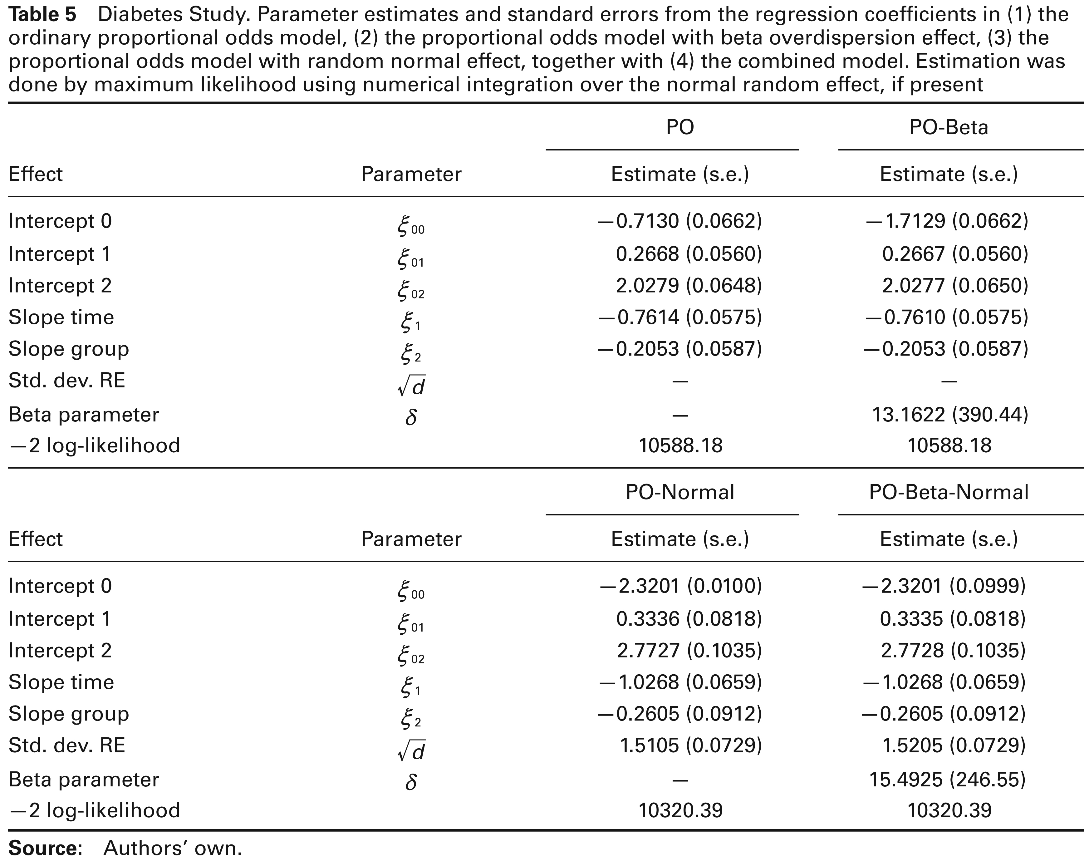
Diabetes Study. Parameter estimates and standard errors from the regression coefficients in (1) the ordinary proportional odds model, (2) the proportional odds model with beta overdispersion effect, (3) the proportional odds model with random normal effect, together with (4) the combined model. Estimation was done by maximum likelihood using numerical integration over the normal random effect, if present

Effect	Parameter	PO	PO-Beta
Effect	Parameter	Estimate (s.e.)	Estimate (s.e.)
Intercept 0	$_{00}$	—0.7130 (0.0662)	—1.7129 (0.0662)
Intercept 1	$_{01}$	0.2668 (0.0560)	0.2667 (0.0560)
Intercept 2	$_{02}$	2.0279 (0.0648)	2.0277 (0.0650)
Slope time	$_{1}$	—0.7614 (0.0575)	—0.7610 (0.0575)
Slope group	$_{2}$	—0.2053 (0.0587)	—0.2053 (0.0587)
Std. dev. RE	$\sqrt{d}$	—	—
Beta parameter		—	13.1622 (390.44)
—2 log-likelihood		10588.18	10588.18
Effect	Parameter	PO-Normal	PO-Beta-Normal
Effect	Parameter	Estimate (s.e.)	Estimate (s.e.)
Intercept 0	$_{00}$	—2.3201 (0.0100)	—2.3201 (0.0999)
Intercept 1	$_{01}$	0.3336 (0.0818)	0.3335 (0.0818)
Intercept 2	$_{02}$	2.7727 (0.1035)	2.7728 (0.1035)
Slope time	$_{1}$	—1.0268 (0.0659)	—1.0268 (0.0659)
Slope group	$_{2}$	—0.2605 (0.0912)	—0.2605 (0.0912)
Std. dev. RE	$\sqrt{d}$	1.5105 (0.0729)	1.5205 (0.0729)
Beta parameter		—	15.4925 (246.55)
—2 log-likelihood		10320.39	10320.39

Source: Authors’ own.

7 Concluding remarks

In this article, we have proposed a model for overdispersed, repeated ordinal data. The model combines the proportional odds assumption to handle the ordinal nature of the outcome, with normal random effects in the linear predictor to deal with correlation across repeated measures, and beta random effects to account for overdispersion. Similar models had been proposed by MVD, MVDV, and MVID, for count data, binary and binomial data, and time-to-event outcomes. Ordinal outcomes seem a logical extension, but the ordinal nature of the outcome is generally handled by replacing it with a set of non-redundant indicator variables. This adds a layer of complexity to the modelling process that had not been studied earlier.

The model is easy to formulate and can be fitted in almost a routine fashion using, for example, the SAS procedure NLMIXED. Example code is provided and briefly discussed in the Appendix.

We applied the method to two sets of data, with quite different results. In the diabetes study, there clearly is no need for an overdispersion random effect, so that the conventional generalized linear mixed model, the PO-Normal model in this instance, suffices. For the fluvoxamine trial the situation is different and presents a peculiarity. First comparing the univariate PO model with the PO-Beta model for overdispersion seems to suggest that there no overdispersion is present in the data. However, comparing the PO model with the PO-Normal model suggests that there is a need for normal random effects, which is not surprising given the longitudinal design. Once accounting for the normal random effects, strong evidence is found in favour of overdispersion, when comparing the PO-Normal to the PO-Beta-Normal model. The conclusion is that a forward selection on these sources of variability is not the best route. Instead, a backward selection procedure is advisable, where the more complex model, i.e., the PO-Beta-Normal model, is fitted first. The consequence is that one better starts with the model correcting for overdispersion in addition to correcting for correlation. In other words, a combined model such as the PO-Beta-Normal model would have to be considered more, and more routinely, than is currently the case.

Footnotes

Acknowledgements

Financial support from the IAP research network #P7/06 of the Belgian Government (Belgian Science Policy) is gratefully acknowledged.

SAS implementation

By way of example code, we will illustrate the procedures for the case of four time points per subject. These procedures can simply be reformulated by the user to the case of different numbers of time points, and different numbers of categories per ordinal outcome.

We use the following instance of the NLMIXED procedure in SAS, for the proportional odds model with normal random effect. In line with Molenberghs and Verbeke (2005, Ch. 18) the programme makes use of so-called general-likelihood feature, i.e., a user-defined likelihood that can be applied with the ‘general()’ option in the MODEL statement: proc nlmixed data=fluvo qpoints=10; parms int0=–2 int1=1 int2=3 beta11=1.5 beta12=3 beta13=4 beta2=–0.5 beta3=–0.1 beta4=–0.5 beta5=–0.1 sigma=1; title “Proportional Odds with Normal Random Effect”; eta = b + beta11*t1 + beta12*t2 + beta13*t3 + beta2*anteced + beta3*age1 + beta4*duration1 + beta5*severit0; if theff = 0 then lik = exp(int0+eta)/(1+exp(int0+eta)); else if theff = 1 then lik = exp(int1+eta)/(1+exp(int1+eta)) – exp(int0+eta)/(1+exp(int0+eta)); else if theff = 2 then lik = exp(int2+eta)/(1+exp(int2+eta)) – exp(int1+eta)/(1+exp(int1+eta)); else if theff = 3 then lik = 1 – exp(int2+eta)/(1+exp(int2+eta)); loglik = log(lik); model theff ~ general(loglik); random b ~ normal(0, sigma**2) subject = patient; run;

Similar logic in programming the model was followed by Booth et al. (2003). For a given data analysis, it is best to let the number of quadrature points (‘qpoint=’ option) be decided using a numerical sensitivity analysis. This is easily done by progressively letting the number of quadrature points increase, until parameter estimates and all related quantities (including standard errors, log-likelihood at maximum, etc.) stabilize.

The special case of the proportional odds model, without random effects, simply is obtained by removing the RANDOM statement, and by excluding the random intercept: proc nlmixed data=fluvo; parms int0=–2 int1=1 int2=3 beta11=1.5 beta12=3 beta13=4 beta2=–0.5 beta3=–0.1 beta4=–0.5 beta5=–0.1; title “Proportional Odds without Random Effects”; eta = beta11*t1 + beta12*t2 + beta13*t3 + beta2*anteced + beta3*age1 + beta4*duration1 + beta5*severit0; if theff = 0 then lik = exp(int0+eta)/(1+exp(int0+eta)); else if theff = 1 then lik = exp(int1+eta)/(1+exp(int1+eta)) – exp(int0+eta)/(1+exp(int0+eta)); else if theff = 2 then lik = exp(int2+eta)/(1+exp(int2+eta)) – exp(int1+eta)/(1+exp(int1+eta)); else if theff = 3 then lik = 1 – exp(int2+eta)/(1+exp(int2+eta)); loglik = log(lik); model theff ~ general(loglik); run;

The general likelihood feature is also ideally suited to implement the combined models. The following SAS code is an example of this for a proportional combined odds model: proc nlmixed data=fluvo qpoints=10; parms int0=–2 int1=1 int2=3 beta11=1.5 beta12=3 beta13=4 beta2=–0.5 beta3=–0.1 beta4=–0.5 beta5=–0.1 delta=0.1 sigma=1; title “Proportional Odds With Beta and Normal Random Effects”; eta = beta11*t1 + beta12*t2 + beta13*t3 + beta2*anteced + beta3*age1 + beta4*duration1 + beta5*severit0 + b; nu=exp(delta)/(1+exp(delta)); if theff = 0 then lik = nu*exp(int0+eta)/(1+exp(int0+eta)); else if theff = 1 then lik = nu*exp(int1+eta)/(1+exp(int1+eta)) – nu*exp(int0+eta)/(1+exp(int0+eta)); else if theff = 2 then lik = nu*exp(int2+eta)/(1+exp(int2+eta)) – nu*exp(int1+eta)/(1+exp(int1+eta)); else if theff = 3 then lik = 1 – nu*exp(int2+eta)/(1+exp(int2+eta)); loglik = log(lik); model theff ~ general(loglik); random b ~ normal(0, sigma**2) subject = patient; run;

The combined model is relatively easy to implement and certainly of the same order of programming complexity as the classical proportional odds model with random effect.

References

Agresti

(2002) Categorical Data Analysis, 2nd edition. New York: John Wiley & Sons.

Booth

Casella

Friedl

Hobert

(2003) Negative binomial loglinear mixed models. Statistical Modelling, 3, 179–81.

Borgermans

Goderis

Van Den Broeke

Verbeke

Carbonez

Ivanova

Mathieu

Aertgeerts

Heyrman

Grol

(2009) Interdisciplinary diabetes care Teams operating on the interface between primary and specialty care are associated with improved outcomes of care: Findings from the Leuven Diabetes Project. BMC Health Services Research, 9, 179.

Breslow

Clayton

(1993) Approximate inference in generalized linear mixed models. Journal of the American statistical Association, 88, 9–25.

Cox

Hinkley

(1974) Theoretical statistics. London: Chapman & Hall/CRC.

Engel

Keen

(1994) A simple approach for the analysis of generalized linear mixed models. Statistica Neerlandica, 48, 1–22.

Hinde

Demétrio

CGB

(1998a) Over-dispersion: Models and estimation. Computational Statistics and Data Analysis, 27, 151–70.

Hinde

Demétrio

CGB

(1998b) Overdispersion: Models and estimation. São Paulo: XIII Sinape.

Jørgensen

(1987) Exponential dispersion models. Journal of the Royal Statistical Society, Series B, 49, 127–62.

10.

Kenward

Lesaffre

Molenberghs

(1994) An application of maximum likelihood and generalized estimating equations to the analysis of ordinal data from a longitudinal study with cases missing at random. Biometrics, 50, 945–53.

11.

Lee

Nelder

Pawitan

(2006) Generalized linear models with random effects: unified analysis via H-likelihood. Boca Raton: Chapman & Hall/CRC.

12.

McCullagh

Nelder

(1989) Generalized linear models. London: Chapman & Hall/CRC.

13.

Michiels

Molenberghs

(1997) Protective estimation of longitudinal categorical data with nonrandom dropout. Communications in Statistics, Theory and Methods, 26, 65–94.

14.

Molenberghs

Kenward

Lesaffre

(1997) The analysis of longitudinal ordinal data with non-random dropout. Biometrika, 84, 33–44.

15.

Molenberghs

Lesaffre

(1994) Marginal modelling of correlated ordinal data using a multivariate Plackett distribution. Journal of the American Statistical Association, 89, 633–44.

16.

Molenberghs

Verbeke

(2005) Models for discrete longitudinal data. New York: Springer.

17.

Molenberghs

Verbeke

(2007) Likelihood ratio, score, and Wald tests in a constrained parameter space. The American Statistician, 61, 1–6.

18.

Molenberghs

Verbeke

Demétrio

CGB

(2007) An extended random-effects approach to modeling repeated, overdispersed count data. Lifetime Data Analysis, 13, 513–31.

19.

Molenberghs

Verbeke

Demétrio

CGB

Vieira

(2010) A family of generalized linear models for repeated measures with normal and conjugate random effects. Statistical Science, 25, 325–47.

20.

Molenberghs

Verbeke

Iddi

Demétrio

CGB

(2012) A combined beta and normal random-effects model for repeated, overdispersed binary and binomial data. Journal of Multivariate Analysis, 111, 94–109.

21.

Nelder

Wedderburn

RWM

(1972) Generalized linear models. Journal of the Royal Statistical Society, Series B, 135, 370–84.

22.

Self

Liang

(1987) Asymptotic properties of maximum likelihood estimators and likelihood ratio tests under nonstandard conditions. Journal of the American Statistical Association, 82, 605–10.

23.

Stram

Lee

(1994) Variance components testing in the longitudinal mixed effects model. Biometrics, 50, 1171–77.

24.

Stram

Lee

(1995) Correction to: Variance components testing in the longitudinal mixed effects model. Biometrics, 51, 1196.

25.

Verbeke

Molenberghs

(2000) Linear mixed models for longitudinal data. New York: Springer-Verlag.

26.

Verbeke

Molenberghs

(2003) The use of score tests for inference on variance components. Biometrics, 59, 254–62.

27.

Wolfinger

O’Connell

(1993) Generalized linear mixed models: A pseudo-likelihood approach. Journal of Statistical Computation and Simulation, 48, 233–43.

# Clin. Targets	# Observations
	T₀		T₁
	UQIP	AQIP	UQIP	AQIP
0	116 (14.8%)	191 (14.0%)	54 (7.2%)	74 (5.6%)
1	314 (40.2%)	514 (37.8%)	238 (31.8%)	360 (27.4%)
2	259 (33.1%)	467 (34.3%)	304 (40.6%)	530 (40.4%)
3	93 (11.9%)	188 (13.8%)	152 (20.3%)	349 (26.6%)
Total	782	1360	748	1313