Subject-specific Bradley–Terry–Luce models with implicit variable selection

Abstract

The Bradley–Terry–Luce (BTL) model for paired comparison data is able to obtain a ranking of the objects that are compared pairwise by subjects. The task of each subject is to make preference decisions in favour of one of the objects. This decision is binary when subjects prefer either the first object or the second object, but can also be ordinal when subjects make their decisions on more than two preference categories. Since subject-specific covariates, which reflect characteristics of the subject, may affect the preference decision, it is essential to incorporate subject-specific covariates into the model. However, the inclusion of subject-specific covariates yields a model that contains many parameters and thus estimation becomes challenging. To overcome this problem, we propose a procedure that is able to select and estimate only relevant variables.

Keywords

boosting Bradley–Terry–Luce model Paired comparison subject-specific covariate variable selection

1 Introduction

In paired comparisons, several objects are compared pairwise to obtain an overall preference ranking of the objects. In many application fields, such as, marketing research or psychometric experiments, objects are presented in a pairwise manner to judges, or, as they are called here, subjects. Their task for each comparison is to make a preference decision in favour of one of the presented objects according to specific subjective criteria, for example, the fragrance of perfumes when two perfumes are the objects being compared. Subjects can typically choose to prefer either the first or the second object, so that the response is represented by a binary variable. Alternatively, the subjects can make their preference decisions on more than two preference categories, such as, preferring the first object strongly or weakly, preferring neither of the objects, or preferring the second object strongly or weakly. This procedure yields an ordinal response that allows for a more precise preference ranking of the objects because it uses additional information about how strongly an object is preferred.

One of the most widely used models for paired comparisons with a binary response is the model suggested by Bradley and Terry (1952). It is closely related to the choice axiom of Luce (1959) with the restriction of choices to between two objects. Thus, the model is also known as Bradley–Terry–Luce (BTL) model. Several extensions have been proposed in the literature to allow for responses with more than two preference categories. The former approaches allowed only a third category and were proposed by Rao and Kupper (1967) and Davidson (1970). Later, ordinal BTL models that allow for any number of ordered response categories were considered by Tutz (1986), Agresti (1992), Dittrich et. al. (2004)) and Dittrich et. al.(2007). Ordinal regression models, in particular the cumulative logit model and the adjacent categories logit model, are in common use when an ordinal response is present. The models presented in this paper assume independence among all observations, so that pairwise ratings from the same subject are modelled as independent. However, in some applications, including a dependence structure is more realistic. In this context, Böckenholt (2001) introduced dependencies among observations by including subject- and object-specific random components.

The main objective of this article is to develop a method that allows for variable selection in a model that also contains subject-specific covariates. These covariates are characteristics of the subject and are assumed to affect the decision of a subject. Selection of relevant subject-specific covariates is very important because subject-specific BTL models typically contain a large number of parameters, and the estimation of all these parameters becomes challenging. Therefore, we focus on detecting important characteristics that determine the preference of objects.

2 Paired comparison models

2.1 The binary BTL model

Let $M$ be the number of objects that are being compared and let the pair $(r, s)$ refer to the comparison of object $r$ and object $s$ . The response connected to this comparison is denoted by $Y_{rs}$ , where $Y_{rs} = 1$ indicat indicates the preference for object r and $Y_{r s} = 2$ indicates the preference for object s. Let $π_{k}^{(r, s)} : = ℙ (Y_{r s} = k | (r, s))$ with k = 1, 2 and $π_{1}^{(r, s)} + π_{2}^{(r, s)} = 1$ denote the probability of whether object r (for k = 1) or object s (for k = 2) is preferred. The binary BTL model can then be written as a logistic model

\begin{matrix} log (π_{1}^{(r, s)} / (1 - π_{1}^{(r, s)})) & = & γ_{r} - γ_{s} \\ = & x_{1}^{(r, s)} γ_{1} + \dots + x_{M - 1}^{(r, s)} γ_{M - 1} \\ = & {(x^{(r, s)})}^{⊤} γ, \end{matrix}

(2.1)

where the components of the vector

{(x^{(r, s)})}^{⊤} = (x_{1}^{(r, s)}, \dots, x_{M - 1}^{(r, s)})

are defined as

x_{m}^{(r, s)} = \{\begin{matrix} + 1 & if m = r \\ - 1 & if m = s \\ 0 & otherwise . \end{matrix}

Given the pair

(r, s)

, the vector

{(x^{(r, s)})}^{⊤} = (0, \dots, 1, 0, \dots, - 1, 0 \dots, 0)

has a

1

on the

r

th position and a

- 1

on the

s

th position. The vector

γ = {(γ_{1}, \dots, γ_{M - 1})}^{⊤}

contains all object parameters that are to be estimated, where each parameter

γ_{m}

reflects the worth of object

m

. For model identifiability, we use the restriction

γ_{M} = 0

, that is, object

M

is considered as reference object. The ranking of objects is based on estimated object parameters, where estimation is carried out by maximum likelihood estimation for ordinary logistic models (Turner and Firth, 2012).

2.2 Ordinal BTL models

In the binary BTL model, the subjects can prefer the first object or the second object of a comparison. In more general settings, the subjects can make their preference decisions on more than two preference categories. In this case, the binary response is extended to a symmetric ordinal response $Y_{rs} \in {1, \dots, K}$ , where $K$ denotes an arbitrary number of response categories. In our notation, lower response categories indicate the preference for object $r$ . Thus, $Y_{rs} = 1$ is the most favourable response category for object $r$ and $Y_{rs} = K$ is the most favourable response category for object $s$ , or, equivalently, the least favourable response category for object $r$ . To ensure that the comparison of the pair $(r, s)$ yields the same result as the comparison of the pair $(s, r)$ , the ordinal response is assumed to be symmetric, that is, $Y_{rs} = k \Leftrightarrow Y_{sr} = K - k + 1$ and therefore $π_{k}^{(r, s)} = π_{K - k + 1}^{(s, r)}$ (Agresti 1992).

2.2.1 The cumulative model

The cumulative BTL model for ordinal responses uses the cumulative probabilities $ℙ (Y_{rs} \leq k | (r, s)) = π_{1}^{(r, s)} + \dots + π_{k}^{(r, s)}$ and $ℙ (Y_{rs} > k | (r, s)) = π_{k + 1}^{(r, s)} + \dots + π_{K}^{(r, s)}$ , with $ℙ (Y_{rs} \leq k | (r, s)) + ℙ (Y_{rs} > k | (r, s)) = π_{1}^{(r, s)} + \dots + π_{K}^{(r, s)} = 1$ . The model can be formulated as a cumulative logit model (McCullagh, 1980) with the link function $g = {(g_{1}, \dots, g_{K - 1})}^{⊤}$ , where

g_{k} (π_{1}^{(r, s)}, \dots, π_{K}^{(r, s)}) = log (\frac{π_{1}^{(r, s)} + \dots + π_{k}^{(r, s)}}{1 - (π_{1}^{(r, s)} + \dots + π_{k}^{(r, s)})})

links the considered probabilities to the linear predictor

η_{k}^{(r, s)}

, so that

\begin{matrix} g_{k} (π_{1}^{(r, s)}, \dots, π_{K}^{(r, s)}) & = & η_{k}^{(r, s)} & = & θ_{k} + (γ_{r} - γ_{s}) \\ = & θ_{k} + (x_{1}^{(r, s)} γ_{1} + \dots + x_{M - 1}^{(r, s)} γ_{M - 1}) \\ = & θ_{k} + {(x^{(r, s)})}^{⊤} γ, \end{matrix}

(2.2)

for all

k = 1, \dots, K - 1

and with the threshold parameters

- \infty = θ_{0} < θ_{1} < \dots < θ_{K - 1} < θ_{K} = \infty

. Because of the symmetric response, the thresholds need to be restricted as follows (see Tutz, 1986):

(1) If $K$ is odd

θ_{k} = - θ_{K - k} for k = 1, \dots, \frac{K - 1}{2} = ⌊\frac{K - 1}{2}⌋ .

(2.3)

(2) If $K$ is even

θ_{K / 2} = 0 and θ_{K / 2 - k} = - θ_{K / 2 + k} for k = 1, \dots, \frac{K}{2} - 1 = ⌊\frac{K - 1}{2}⌋ .

(2.4)

It can be seen that only

q : = ⌊\frac{K - 1}{2}⌋

threshold parameters need to be estimated; the other ones are determined by the symmetry constraints (2.3) and (2.4).

2.2.2 The adjacent categories model

Another model that also allows for ordinal responses is the adjacent categories BTL model. It is based on the adjacent categories logit model using the link function $g = {(g_{1}, \dots, g_{K - 1})}^{⊤}$ , with

g_{k} (π_{1}^{(r, s)}, \dots, π_{K}^{(r, s)}) = log (\frac{π_{k}^{(r, s)}}{π_{k + 1}^{(r, s)}}) .

The model is then defined by

g_{k} (π_{1}^{(r, s)}, \dots, π_{K}^{(r, s)}) = η_{k}^{(r, s)} = θ_{k} + {(x^{(r, s)})}^{⊤} γ, k = 1, \dots, K - 1 .

(2.5)

Here, the same restrictions (2.3) and (2.4) are valid and allow for symmetric thresholds see Agresti, (1992). The adjacent categories BTL model can also be represented as a log-linear model, which has been extensively discussed in the literature (see Agresti 1992; Dittrich et. al., 1998, 2004, 2007). When the response consists of

K = 2

categories, the binary BTL model (2.1) is a special case of the cumulative BTL model (2.2) and the adjacent categories BTL model (2.5). In this case, the cumulative BTL model and the adjacent categories BTL model are equivalent.

It should be noted that the cumulative model and the adjacent categories model for ordinal responses use the same set of linear predictors

η_{k}^{(r, s)} = θ_{k} + {(x^{(r, s)})}^{⊤} γ, k = 1, \dots, q .

(2.6)

Therefore, the inclusion of subject-specific covariates for both models is obtained by modifying the same linear predictors.

3 Including subject-specific covariates

A very restrictive assumption for the models considered in Section 2.2 is that the worth of an object is the same for all subjects. Therefore, the ranking of the objects is the same for all subjects. However, in most applications it is to be expected that the preference for an object and thus the ranking of all objects depends on characteristics of the subject that makes the preference decision (Dittrich et. al., 1998; Francis et. al., 2002). To explicitly model this heterogeneity, we introduce subject-specific covariates $x_{i, 1}, \dots, x_{i, P}$ , which can be both categorical or continuous characteristics of the subject. In this case, $P$ reflects the number of characteristics and $i$ refers to a single subject. The object parameters are now assumed to be determined by these characteristics, such that the object parameters vary across subjects. The resulting object parameter for subject $i$ is then specified by

\begin{matrix} γ_{i, m} = γ_{m} + \sum_{p = 1}^{P} x_{i, p} γ_{m, p}, \end{matrix}

where

γ_{m}

is a parameter for object

m

that is independent of the characteristics of the subject, and

γ_{m, p}

is a modifying effect for object

m

depending on the

p

th subject-specific covariate. This means that

γ_{m, p}

is a subject–object interaction parameter. To ensure model identifiability, we constraint the subject–object interaction parameters by setting

γ_{M, p} = 0

, for all

p = 1, \dots, P

(Francis et. al., 2002). Assuming that there are

i = 1, \dots, I

subjects, the linear predictor

η_{k}^{(r, s)}

from equation (2.6) can be replaced by a more flexible linear predictor

η_{k}^{(r, s), i}

that also considers subject-specific covariates and has the form

\begin{matrix} η_{k}^{(r, s), i} & = & θ_{k} + (γ_{i, r} - γ_{i, s}) & = & θ_{k} + (γ_{r} - γ_{s}) + \sum_{p = 1}^{P} x_{i, p} (γ_{r, p} - γ_{s, p}) \\ = & θ_{k} + \sum_{m = 1}^{M - 1} x_{m}^{(r, s)} γ_{m} + \sum_{p = 1}^{P} \sum_{m = 1}^{M - 1} x_{i, p} x_{m}^{(r, s)} γ_{m, p} \\ = & θ_{k} + {(x^{(r, s)})}^{⊤} γ + \sum_{p = 1}^{P} {(x_{p}^{(r, s), i})}^{⊤} γ_{p} . \end{matrix}

Here, the vector

{(x_{p}^{(r, s), i})}^{⊤} = (x_{i, p} x_{1}^{(r, s)}, \dots, x_{i, p} x_{M - 1}^{(r, s)})

contains all subject–object interactions that belong to the

p

th subject-specific covariate and

γ_{p}^{⊤} = (γ_{1, p}, \dots, γ_{M - 1, p})

is the corresponding vector of subject–object (interaction) parameters, such that

γ_{m, p}

refers to the

m

th object and the

p

th subject-specific covariate.

In the absence of subject-specific covariates, that is, $x_{i, p} = 0$ , for all $i, p$ , one obtains an ordinal BTL model as described previously. The model that considers subject-specific covariates is more flexible and accounts for heterogeneity between subjects but suffers from the large number of parameters. This is because one has to estimate $M - 1$ subject–object parameters, namely, $γ_{p}^{⊤} = (γ_{1, p}, \dots, γ_{M - 1, p})$ , for each additional subject-specific covariate (that is, when $p$ increases by $1$ ). To overcome this problem, we present a component-wise boosting algorithm that implicitly selects the influential variables.

4 Boosting

4.1 Basic concept of boosting

Before introducing the boosting algorithm for ordinal BTL models, we will first illustrate the concept of boosting on a linear regression model and then proceed to boosting for ordinal BTL models.

Assume the linear regression model with $C$ covariates and $J$ observations. In matrix representation, the model can be described as

y = X β + ε,

with the vectors

y = {(y_{1}, \dots, y_{J})}^{⊤}

ε = {(ε_{1}, \dots, ε_{J})}^{⊤}

β = {(β_{0}, \dots, β_{C})}^{⊤}

and the design matrix

X = [x_{0}, x_{1}, \dots, x_{C}]

that contains the components

x_{c} = {(x_{1, c}, \dots, x_{J, c})}^{⊤}

for

c = 0, 1, \dots, C

. The structure of a generalized linear model (GLM) is determined by

μ_{j} = E (y_{j} | x_{j}) = h (η_{j})

, where

h

is a known response function and

g = h^{- 1}

is the link function that links the conditional expectation

E (y_{j} | x_{j})

to the linear predictor

η_{j} = \sum_{c = 0}^{C} x_{j, c} β_{c}

. Using the vectors

μ = {(μ_{1}, \dots, μ_{J})}^{⊤}

and

η = {(η_{1}, \dots, η_{J})}^{⊤}

, we can also write

μ = h (η)

and

g (μ) = η

. The linear model above can be incorporated within the framework of GLMs by using the identity function as the link function, that is,

μ_{j} = g (μ_{j}) = η_{j} = h (η_{j})

. For a large number of covariates

C

, it is of interest to estimate the model using only influential variables. There are several methods that perform well in such high-dimensional settings while offering a sparse model; one of these methods is boosting (see Bühlmann, 2006). Boosting has its origin in the machine learning community (see Schapire 1990; Freund 1995, 1997) and can be formulated within the framework of statistical modelling as iteratively fitting parts of the model using the residuals of the previous iteration as the response of the current iteration (Friedman et. al., 2000; Friedman 2001). The basic concept of boosting is to use a set of so-called base learners

f (\cdot)

and combine them to gain a strong learner. A base learner can be a function of a set of covariates or even a single covariate. In this article, we will consider only linear base learners that are able to express a linear effect of the considered covariate(s). In the linear model, a single linear base learner for the

c

th component is, for example,

f (x_{c}, β_{c}) = x_{c} β_{c} .

Tutz and Binder (2006) introduced likelihood-based boosting for GLMs. Instead of the iteratively refitting of residuals, they used the linear predictor $η^{(b - 1)}$ of the previous iteration $(b - 1)$ as an offset that adds up to the linear predictor $η^{(b)}$ of the current iteration $b$ . We describe a component-wise boosting algorithm, where component-wise means that in each iteration only a single component is considered at a time.

Component-wise Boosting

Step 1: Initialization

Fit the intercept model $μ^{(0)} = h (η^{(0)}) = h (x_{0} β_{0}),$ with $x_{0} = {(x_{1, 0}, \dots, x_{J, 0})}^{⊤} = {(1, \dots, 1)}^{⊤}$ by maximizing the likelihood to obtain the estimated intercept ${\hat{β}}_{0}$ . Initialize

{\hat{β}}^{(0)} = {({\hat{β}}_{0}, {\hat{β}}_{1}, \dots, {\hat{β}}_{C})}^{⊤} = {({\hat{β}}_{0}, 0, \dots, 0)}^{⊤} and {\hat{η}}^{(0)} = x_{0} {\hat{β}}_{0} .

Step 2: For each boosting iteration $b = 1, 2, \dots, b_{} stop$

(a) Estimation: Fit the models

μ = h ({\hat{η}}^{(b - 1)} + f (x_{c}, β_{c}))

for all components

c = 0, \dots, C

by one-step Fisher scoring, where

{\hat{η}}^{(b - 1)}

is used as an offset. This yields the one-step Fisher scoring estimates

{\hat{β}}_{c}

for the corresponding

c

th component. In general, the Fisher scoring algorithm is an iterative estimation procedure and uses the Fisher-matrix and the score function (for more details, see Tutz and Binder 2006).

(b) Selection: From the models fitted in (a), choose the component $c^{*}$ that yields the best fit with respect to some criteria (e.g., the model with the lowest deviance, Akaike information criterion (AIC) or Bayesian information criterion (BIC)) and set

{\hat{β}}_{c^{*}} = {(0, \dots, 0, {\hat{β}}_{c^{*}}, 0, \dots, 0)}^{⊤} .

${\hat{η}}^{(b)} = {\hat{η}}^{(b - 1)} + X {\hat{β}}_{c^{*}}$ , with $X = [x_{0}, x_{1}, \dots, x_{C}]$

${\hat{β}}^{(b)} = {\hat{β}}^{(b - 1)} + {\hat{β}}_{c^{*}}$

4.2 Boosting ordinal BTL models

Boosting ordinal BTL models The boosting algorithm described in this section is a component-wise boosting procedure based on the pomBoost algorithm (Zahid and Tutz, 2013), which has been developed for the cumulative logit model. It allows for ordinal responses and can be extended to the adjacent categories logit model by modifying the link function $g = {(g_{1}, \dots, g_{K - 1})}^{⊤}$ to obtain the adjacent categories logit model (see Section 2.2). We will use a specific feature of the pomBoost algorithm, which allows to split the parameters into two groups to distinguish between obligatory parameters that have to be included in the model and optional parameters that might be of relevance and where a variable selection is applied. In our context, the object parameters $γ^{⊤} = (γ_{1}, \dots, γ_{M - 1})$ are considered as obligatory and the subject-specific parameters $γ_{p}^{⊤} = (γ_{1, p}, \dots, γ_{M - 1, p})$ , for all $p = 1, \dots, P$ are considered as optional. To be more flexible, one can divide the $P$ optional subject-specific covariates into two disjoint sets $V_{grouped}$ and $V_{single}$ , with $V_{grouped} \cup V_{single} = {1, \dots, P}$ . This will allow selection of two different types of covariates, namely,

$V_{grouped}$ : subject-specific covariates, for which all the associated subject–object interactions should be selected simultaneously and

$V_{single}$ : subject-specific covariates, for which all associated subject–object interactions should be selected separately.

The reason for distinguishing these two groups is that for some subject-specific covariates, it might be interesting for the practitioner to have the possibility to select the respective subject–object interactions simultaneously or separately (we refer to the application section for an illustrating example). The subject–object interaction parameters that are associated with the $p$ th subject-specific covariate are given by the set of parameters $γ_{1, p}, \dots, γ_{M - 1, p}$ . If the subject-specific covariate is considered as being from $V_{grouped}$ , the parameters are included as a set or left out, which yields variable selection in terms of the subject-specific covariates. However, if the subject-specific covariate is considered as being from $V_{single}$ , only single parameters from the set are included or left out, which yields selection of subject–object interactions.

The boosting algorithm below uses the design matrix for paired comparisons $X = [Q, X_{0}, X_{1}, \dots, X_{P}]$ , where $Q$ contains the components for the thresholds, $X_{0}$ contains the components for the objects and $X_{1}, \dots, X_{P}$ contain the components for the subject-specific covariates (for more details on the multivariate structure, see Appendix A). Specifically, all matrices $X_{p}$ , with $p = 1, \dots, P$ , have $M - 1$ columns, where each column is denoted by $x_{p, m}$ and reflects a single subject–object interaction between the $p$ th subject-specific covariate and object $m$ . Thus, these matrices have the form $X_{p} = [x_{p, 1}, \dots, x_{p, M - 1}]$ . The algorithm proposed is the following:

BTLboost

Step 1: Initialization

Fit the intercept model $μ^{(0)} = h (η^{(0)}) = h (Q θ)$ by maximizing the likelihood in order to obtain estimates for the threshold parameters $θ = {(θ_{1}, \dots, θ_{q})}^{⊤}$ . Initialize

{\hat{β}}^{(0)} = ({\hat{θ}}^{⊤}, {\hat{γ}}^{⊤}, {\hat{γ}}_{1}^{⊤}, \dots, {\hat{γ}}_{P}^{⊤}) = {({\hat{θ}}_{1}, \dots, {\hat{θ}}_{q}, 0, \dots, 0)}^{⊤} and {\hat{η}}^{(0)} = X {\hat{β}}^{(0)} .

Step 2: For each boosting iteration

b = 1, 2, \dots, b_{stop}

Step 2.1: Update of threshold and object parameters

Estimation: Fit the model $μ = h ({\hat{η}}^{(b - 1)} + Q θ + X_{0} γ)$ by one-step Fisher scoring, where ${\hat{η}}^{(b - 1)}$ is used as an offset. One obtains the estimates ${\hat{θ}}^{⊤} = ({\hat{θ}}_{1}, \dots, {\hat{θ}}_{q})$ , ${\hat{γ}}^{⊤} = ({\hat{γ}}_{1}, \dots, {\hat{γ}}_{M - 1})$ and defines

{\hat{β}}_{0}^{⊤} = ({\hat{θ}}^{⊤}, {\hat{γ}}^{⊤}, {\hat{γ}}_{1}^{⊤}, \dots, {\hat{γ}}_{P}^{⊤}) = ({\hat{θ}}_{1}, \dots, {\hat{θ}}_{q}, {\hat{γ}}_{1}, \dots, {\hat{γ}}_{M - 1}, 0, \dots, 0) .

Update:

${\hat{η}}^{(b)} = {\hat{η}}^{(b - 1)} + X {\hat{β}}_{0}$

${\hat{β}}^{(b)} = {\hat{β}}^{(b - 1)} + {\hat{β}}_{0}$

Step 2.2: Update of parameters for the optional covariates

(a) Estimation: For each subject-specific covariate $p = 1, \dots, P$ , fit the models

μ = \{\begin{matrix} h ({\hat{η}}^{(b)} + X_{p} γ_{p}) & if p \in V_{grouped} \\ h ({\hat{η}}^{(b)} + x_{p, m} γ_{m, p}), \forall m \in {1, \dots, M - 1} & if p \in V_{single} \end{matrix},

where

{\hat{η}}^{(b)}

is used as offset. The estimated parameters

{\hat{γ}}_{p}

and

{\hat{γ}}_{m, p}

are obtained by one-step Fisher scoring.

(b) Selection: From the models fitted in (a), choose the model that maximally improves the fit with respect to some criteria (e.g., deviance, AIC or BIC) and set $X_{best} = x_{p^{*}, m^{*}}$ if the $(p^{*}, m^{*})$ -th subject–object interaction yields the best fit or $X_{best} = X_{p^{*}}$ if the set of subject–object interactions associated with the $p^{*}$ -th subject-specific covariate yields the best fit. This yields the estimated parameter vector

{\hat{β}}_{best}^{⊤} = ({\hat{θ}}^{⊤}, {\hat{γ}}^{⊤}, {\hat{γ}}_{1}^{⊤}, \dots, {\hat{γ}}_{P}^{⊤}) = \{\begin{matrix} (0, \dots, 0, {\hat{γ}}_{p^{*}, m^{*}}, 0, \dots, 0) & if X_{best} = x_{p^{*}, m^{*}} \\ (0, \dots, 0, {\hat{γ}}_{p^{*}}^{⊤}, 0, \dots, 0) & if X_{best} = X_{p^{*}} \end{matrix} .

${\hat{η}}^{(b)} = {\hat{η}}^{(b)} + X {\hat{β}}_{best}$

${\hat{β}}^{(b)} = {\hat{β}}^{(b)} + {\hat{β}}_{best}$

Within each boosting iteration, the algorithm switches between two stages. The first stage (Step $2.1$ ) considers only the object parameters along with the threshold parameters for an update, so that these parameters will always be part of the paired comparison model. In the second stage (Step $2.2$ ), we consider the subject-specific covariates that might enter into the paired comparison model. If the associated subject–object interactions are to be selected simultaneously ( $p \in V_{grouped}$ ), the full subject-specific parameter vector $γ_{p}$ is updated. If they are to be selected separately ( $p \in V_{single}$ ), only a single subject–object interaction parameter $γ_{p, m}$ from the full subject-specific parameter $γ_{p}^{⊤} = (γ_{1, p}, \dots, γ_{M - 1, p})$ is updated within each boosting iteration. This procedure is repeated until a predefined number of boosting iterations $b_{stop}$ is reached. In the next section, we discuss how the optimal number of boosting iterations can be obtained.

4.3 Stopping criteria

The number of boosting iterations $b_{stop}$ is the main tuning parameter in boosting. Typically, a sufficiently high number of iterations is chosen; the optimal number of iterations $b_{stop}^{*}$ is then determined afterwards. Common choices for determining $b_{stop}^{*}$ are either information criteria, such as, the AIC or BIC, or cross-validation. In this paper, we consider only the two information criteria mentioned earlier, which are known measures for the trade-off between goodness-of-fit and model complexity. The computation of both criteria is based on the deviance $Dev ({\hat{η}}^{(b)})$ and the degrees of freedom $df (b)$ after $b$ boosting iterations.

The AIC and BIC after $b$ iterations are given by

AIC (b) = Dev ({\hat{η}}^{(b)}) + 2 \cdot df (b)

and

BIC (b) = Dev ({\hat{η}}^{(b)}) + log (n) \cdot df (b),

where

n

is the number of observations, or, in our case, the number of comparisons that are made by all subjects, namely,

n = (\begin{matrix} M \\ 2 \end{matrix})

. The penalty term, which is

2

for the AIC and

log (n)

for the BIC, controls the model complexity, so that, in general, higher values for the penalty term result in sparser models.

Since the boosting algorithm is an iterative procedure, the true degrees of freedom $df (b)$ after $b$ boosting iterations are unknown and need to be approximated. In the literature, it is often suggested to use the trace of the hat matrix after $b$ boosting iterations as an approximation for the degrees of freedom (Tutz and Binder, 2006; Bühlmann and Hothorn, 2007a). Thus, a possible approximation of the degrees of freedom $df (b)$ is given by

{df}_{trace} (b) = trace (H_{b}),

where

H_{b}

is the approximate hat matrix after

b

iterations. A detailed derivation of the formula for this hat matrix can be found in Zahid and Tutz (2013).

An alternative, computationally simpler method proposed by Bühlmann and Hothorn (2007b) uses the size of the active set, which corresponds to the number of non-zero parameters in the $b$ th boosting iteration, in order to approximate the degrees of freedom $df (b)$ . In this case, the number of non-zero coefficients until the $b$ th boosting iteration is given by

{df}_{actset} (b) = q + (M - 1) + \sum_{m, p}^{} I ({\hat{γ}}_{m, p}^{(b)} \neq 0),

(4.1)

where

q

is the number of threshold parameters,

M - 1

is the number of object parameters,

{\hat{γ}}_{m, p}^{(b)}

are all non-zero subject–object parameters of the

b

th iteration, and

I (\cdot)

is the indicator function, such that

I (\cdot) = 1

if the expression

(\cdot)

is true, else

I (\cdot) = 0

. To limit the computational burden, we use this more convenient method to approximate the degrees of freedom in the simulation and application section.

The optimal stopping iteration $b_{stop}^{*}$ is chosen from among the iterations $b = 1, \dots, b_{stop}$ as the one yielding the best (=lowest) $AIC$ or $BIC$ , respectively. Thus, one has to compute the AIC or BIC for all iterations. The optimal stopping iteration is then determined afterwards using

b_{stop}^{*} = b \Leftrightarrow AIC (b_{stop}^{*}) = min_{b = 1, \dots, b_{stop}} AIC (b),

when the AIC is chosen as stopping criterion or

b_{stop}^{*} = b \Leftrightarrow BIC (b_{stop}^{*}) = min_{b = 1, \dots, b_{stop}} BIC (b),

when the BIC is chosen as stopping criterion, respectively.

5 Simulation

5.1 Simulation set-up

We investigate the performance of the boosting algorithm for different simulation settings with $100$ simulations for each setting. For the simulated data, we generate $20$ subject-specific covariates denoted by $p = 1, \dots, 20$ from the following distributions $X_{1}, \dots, X_{10} \sim B (1, 0.5)$ and $X_{11}, \dots, X_{20} \sim N (0, 1)$ and use $M = 6$ objects that have to be compared by $I = 200$ subjects. We use $K = 3$ response categories, so that each simulated subject has the possibility to prefer the first object, neither of the objects or the second object. In all settings, the ordinal response is computed by assuming an underlying cumulative BTL model with the linear predictor

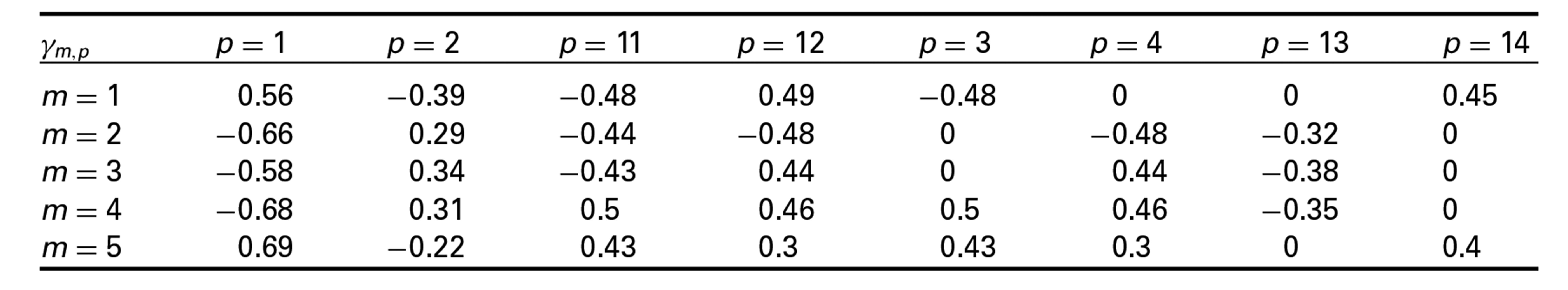
η_{k}^{(r, s), i} = θ_{k} + \sum_{m = 1}^{M - 1} x_{m}^{(r, s)} γ_{m} + \sum_{p = 1}^{P} \sum_{m = 1}^{M - 1} x_{i, p} x_{m}^{(r, s)} γ_{m, p}, k = 1, 2,

using the threshold parameters

θ_{1} = - θ_{2} = - 0.8

and the object parameters

γ = {(γ_{1}, \dots, γ_{M - 1})}^{⊤} = {(1.5, 1.1, 0.7, - 0.7, - 1)}^{⊤}

. The settings are organized as follows.

Setting 1: Only the subject-specific covariates $p = 1, 2, 11, 12$ are influential (parameter values can be obtained from Table 1), while all other subject-specific covariates are non-influential. For each subject-specific covariate, the associated subject–object interactions are selected simultaneously, that is, $V_{grouped} = {1, \dots, 20}$ and $V_{single} = \emptyset$ .

Table 1
Influential subject–object interaction parameters.

$γ_{m, p}$	$p = 1$	$p = 2$	$p = 11$	$p = 12$	$p = 3$	$p = 4$	$p = 13$	$p = 14$
$m = 1$	0.56	$-$ 0.39	$-$ 0.48	0.49	$-$ 0.48	0	0	0.45
$m = 2$	$-$ 0.66	0.29	$-$ 0.44	$-$ 0.48	0	$-$ 0.48	$-$ 0.32	0
$m = 3$	$-$ 0.58	0.34	$-$ 0.43	0.44	0	0.44	$-$ 0.38	0
$m = 4$	$-$ 0.68	0.31	0.5	0.46	0.5	0.46	$-$ 0.35	0
$m = 5$	0.69	$-$ 0.22	0.43	0.3	0.43	0.3	0	0.4

Source: Authors' computation.

Setting 2: Only the subject-specific covariates $p = 3, 4, 13, 14$ are influential (parameter values can be obtained from Table 1). For each subject-specific covariate, the associated subject–object interactions are selected separately, that is, $V_{grouped} = \emptyset$ and $V_{single} = {1, \dots, 20}$ .

Setting 3: In this setting, we consider a miss-specified model. That is, after computing the ordinal response using the influential subject-specific covariates $p = 1, 2, 3, 4, 11, 12, 13, 14$ with the associated parameter values from Table 1, some influential subject-specific covariates were removed from the simulated data set:

(a) The covariates $p = 3, 4, 13, 14$ were removed and the boosting algorithm was applied as in Setting 1, that is, the subject–object interactions for each subject-specific covariate were selected simultaneously, so that all considered covariates are from $V_{grouped}$ .

(b) The covariates $p = 1, 2, 11, 12$ were removed and the boosting algorithm was applied as in Setting 2, that is, the subject–object interactions for each subject-specific covariate were selected separately, so that all considered covariates are from $V_{single}$ .

Setting 4: Same as Setting 1, except that only one subject-specific covariate, $p = 1$ , is considered as influential.

Setting 5: Same as Setting 2, except that only one subject-specific covariate, $p = 3$ , is considered as influential.

As variable selection criterion in each boosting iteration, we use the deviance, which often yields the fully saturated model when the stopping iteration is sufficiently high, i.e., $b_{stop} \to \infty$ (see Bühlmann and Yu, 2003). Therefore, there is a need for determining the optimal number of iterations $b_{stop}^{*}$ using a stopping criterion that chooses the best model among all iterations. In the next section, we compare the results when the AIC and BIC are used as stopping criteria. The degrees of freedoms for the computation of the AIC and BIC are approximated as in equation (4.1).

5.2 Results

Results To investigate the performance of the algorithm, we compute the hit rate

H R = \frac{\sum_{p = 1}^{p} \sum_{m = 1}^{M - 1} I (γ_{m, p} \neq 0) \cdot I ({\hat{γ}}_{m, p} \neq 0)}{\sum_{p = 1}^{p} \sum_{m = 1}^{M - 1} I (γ_{m, p} \neq 0)},

which represents the percentage of correctly identified influential subject–object interactions, and the false alarm rate

F A R = \frac{\sum_{p = 1}^{p} \sum_{m = 1}^{M - 1} I (γ_{m, p} = 0) \cdot I ({\hat{γ}}_{m, p} \neq 0)}{\sum_{p = 1}^{p} \sum_{m = 1}^{M - 1} I (γ_{m, p} = 0)},

which represents the percentage of non-influential subject–object interactions that are mistakenly identified as influential subject–object interactions. The closer the hit rate to 1 and the closer the false alarm rate to 0, the better, because then the model contains many influential subject–object interactions and few non-influential subject–object interactions at the same time.

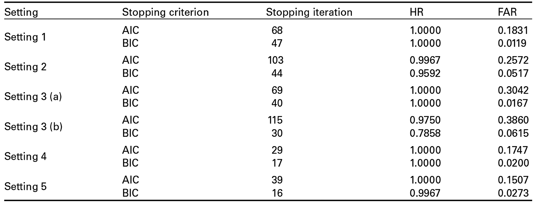
Table 2 shows the averaged number of boosting iterations, as well as the averaged hit rates and false alarm rates over all $100$ simulations in each setting. As the model complexity is supposed to be penalized stronger by the BIC, one sees an earlier stopping of the boosting algorithm when using the BIC instead of the AIC. Except for Setting 2 and Setting 3 (b), the hit rates for the AIC and BIC are very similar and close to 1, that is, the boosting algorithm was always able to identify all (or almost all when using the BIC in Setting 5) influential covariates for Settings 1, 3 (a), 4 and 5. However, at the same time, using the BIC yields a much lower false alarm rate suggesting that using the BIC is more appropriate. In Setting 2, we have a slightly higher hit rate when the AIC is used (the difference in the hit rates is $0.9967 - 0.9592 = 0.0375$ ). However, the false alarm rate is almost five times higher when the AIC is used instead of the BIC ( $0.2572$ compared to $0.0517$ ). Using the AIC in Setting 3 (a) yields a higher hit rate, where the difference in the hit rates is $0.975 - 0.7858 = 0.1892$ . At the same time, the false alarm rate is much worse ( $0.3860$ for the AIC and $0.0615$ for the BIC). Thus, the question of whether the AIC or BIC should be used depends on whether one is interested in identifying most of the influential subject–object interactions (then the AIC might be more appropriate) or in identifying many influential subject–object interactions and few non-influential subject–object interactions at the same time (then the BIC might be more appropriate). In all settings, the false alarm rate is much higher when the AIC is used instead of the BIC. This suggests that more non-influential subject–object interactions are included in the final model determined by the AIC.

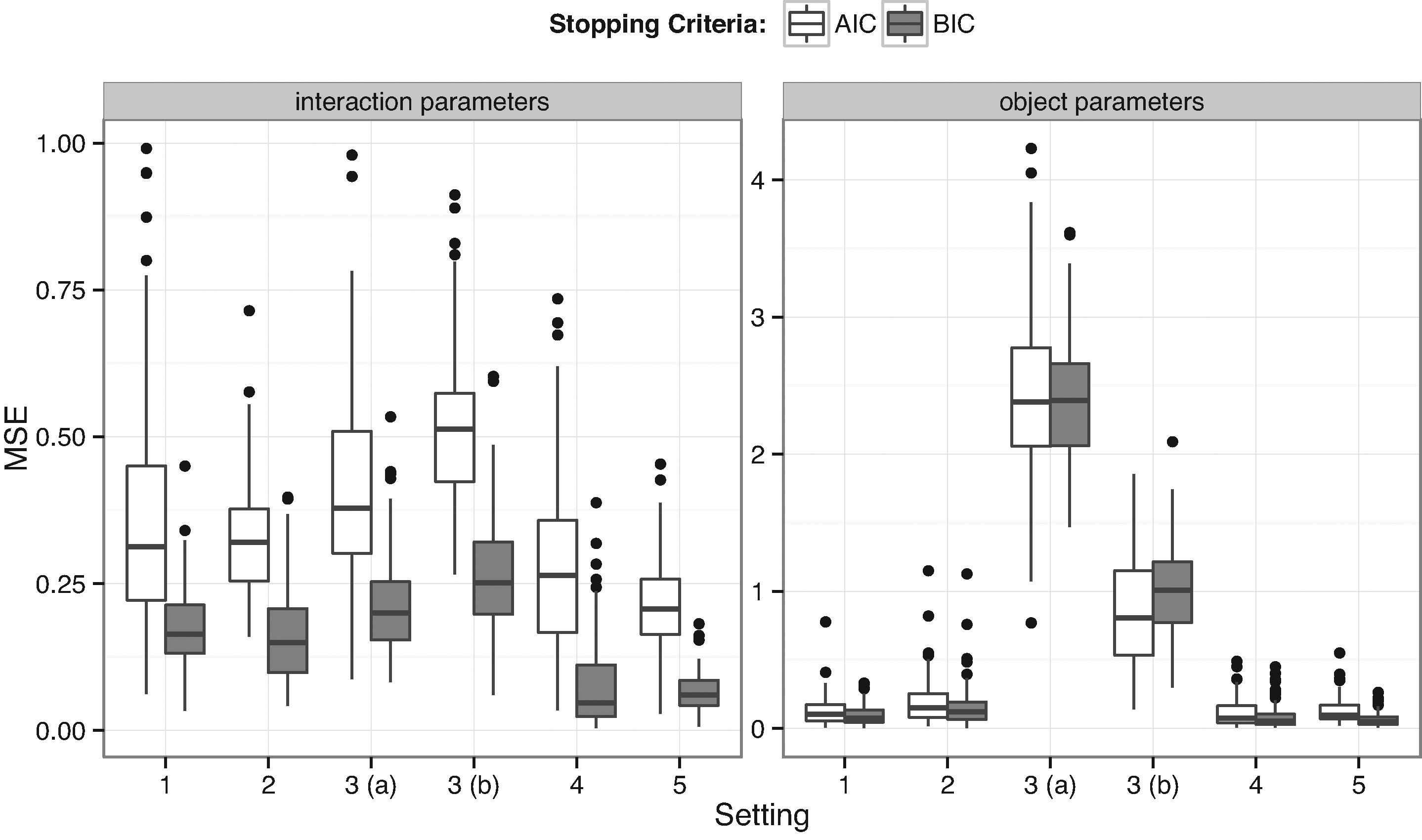
To measure the discrepancy of the parameter estimates with the true parameter values, we use the Mean squared error (MSE). Before computing the MSE for the final model, a final refitting step using the selected subject–object interaction parameters is done. Figure 1 displays the MSE for all simulations and suggests that for the selected subject–object interaction parameters the BIC performs better than the AIC because of smaller MSEs in all settings. It can also be seen that in Setting 3, where a miss-specified model is considered, the MSEs are much larger for the object parameters than for the selected subject–object interaction parameters as compared to the other settings.

Table 2
Average of the HR, the FAR and the number of boosting iterations.

Setting Stopping criterion Stopping iteration HR FAR

Setting 1 AIC 68 1.0000 0.1831

BIC 47 1.0000 0.0119

Setting 2 AIC 103 0.9967 0.2572

BIC 44 0.9592 0.0517

Setting 3 (a) AIC 69 1.0000 0.3042

BIC 40 1.0000 0.0167

Setting 3 (b) AIC 115 0.9750 0.3860

BIC 30 0.7858 0.0615

Setting 4 AIC 29 1.0000 0.1747

BIC 17 1.0000 0.0200

Setting 5 AIC 39 1.0000 0.1507

BIC 16 0.9967 0.0273

Setting	Stopping criterion	Stopping iteration	HR	FAR
Setting 1	AIC	68	1.0000	0.1831
	BIC	47	1.0000	0.0119
Setting 2	AIC	103	0.9967	0.2572
BIC	44	0.9592	0.0517
Setting 3 (a)	AIC	69	1.0000	0.3042
BIC	40	1.0000	0.0167
Setting 3 (b)	AIC	115	0.9750	0.3860
BIC	30	0.7858	0.0615
Setting 4	AIC	29	1.0000	0.1747
BIC	17	1.0000	0.0200
Setting 5	AIC	39	1.0000	0.1507
BIC	16	0.9967	0.0273

Source: Authors' computation.

Figure 1

Source: Authors' computation.

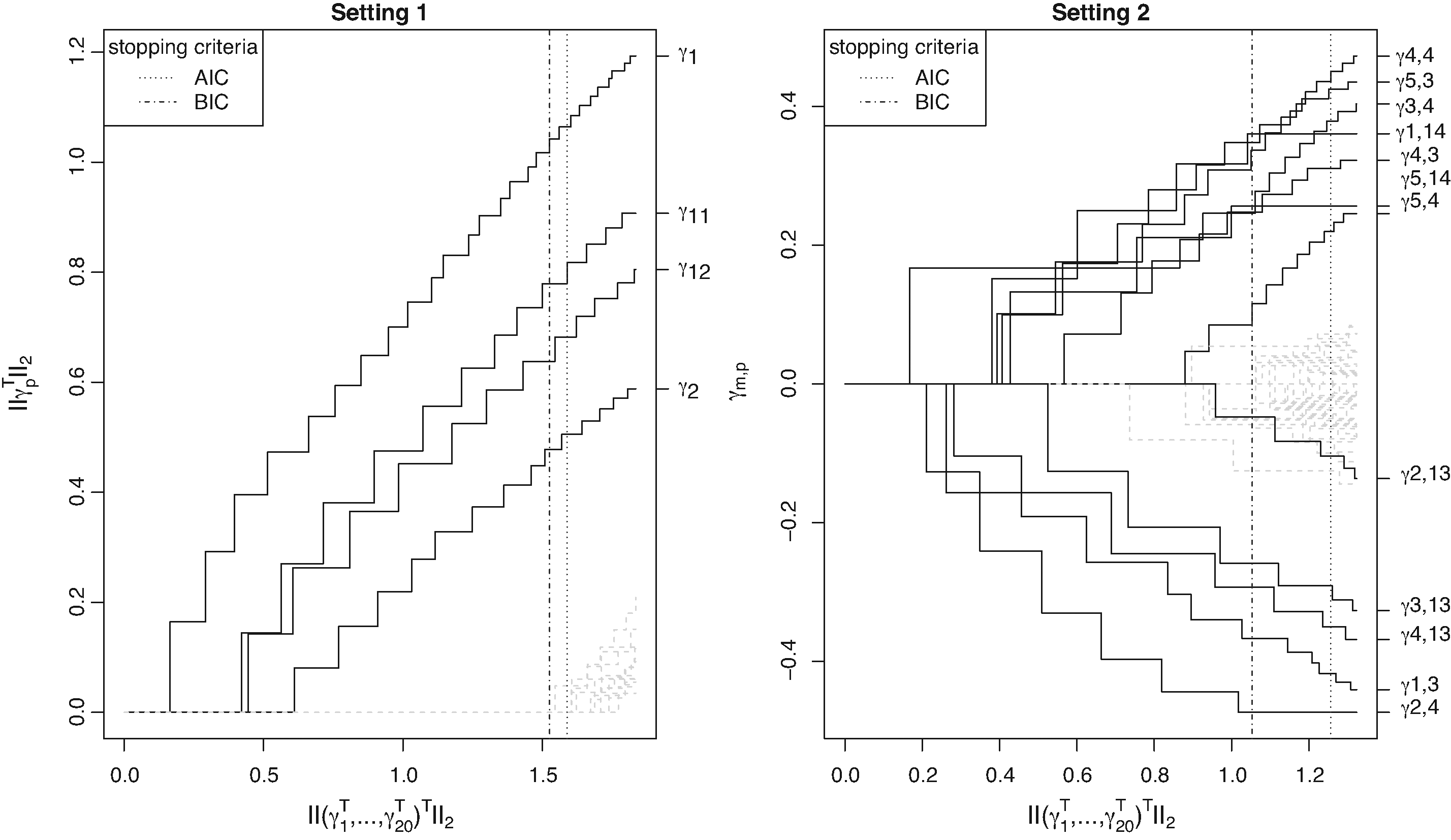
Figure 2 illustrates an exemplary coefficient build-up of the estimated parameters for one out of the $100$ simulations of Setting 1 and Setting 2. Within each boosting iteration of Setting 1 (left figure), the set of subject–object interaction parameters associated with a single subject-specific covariate are updated. Therefore, the norm of a single subject-specific parameter vector $| | {\hat{γ}}_{p}^{⊤} | |$ for each of the $p = 1, \dots, 20$ covariates is plotted against the norm of the parameter vector containing all subject–object parameters $| | {({\hat{γ}}_{1}^{⊤}, \dots, {\hat{γ}}_{20}^{⊤})}^{⊤} | |$ . Conversely, in Setting 2 (right figure) only the parameter of a single subject–object interaction is updated within each boosting iteration. Therefore, the estimates for a single subject–object interaction parameter ${\hat{γ}}_{m, p}$ are plotted against the norm of the parameter vector containing all subject–object parameters $| | {({\hat{γ}}_{1}^{⊤}, \dots, {\hat{γ}}_{20}^{⊤})}^{⊤} | |$ . The coefficient paths show that the non-influential subject–object interaction parameters (dashed gray lines) enter the model in higher boosting iterations and their parameter estimates are small because they are either selected and updated in higher boosting iterations, or they are updated only a few number of times. Since the AIC determines a higher optimal boosting iteration than the BIC, the figure confirms that the final model based on the AIC criterion contains more non-influential subject–object interactions than the final model based on the BIC criterion.

Figure 2

Source: Authors' computation.

6 CEMS data

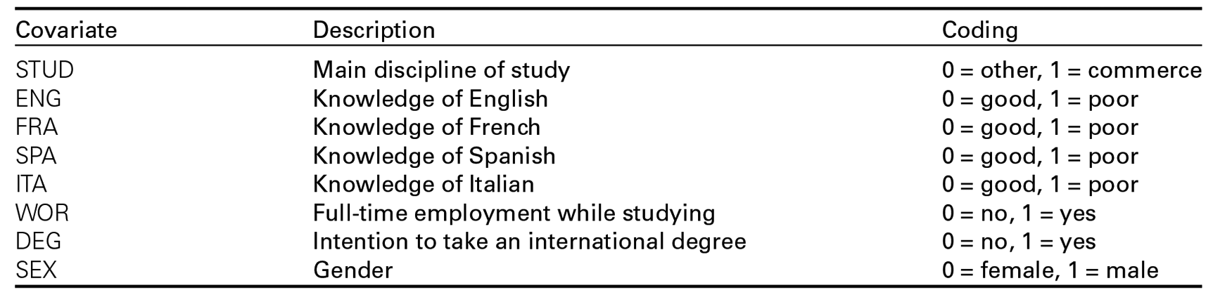
6CEMS data To illustrate how the variable selection method works, we use the Community of European management schools (CEMS) data from Dittrich et. al. (1998), which was collected in a survey of $303$ students of the Vienna University of Economics. The aim of the study was to investigate the preferences of students for studying at least one semester abroad in one of six different universities (London, Paris, Barcelona, St.Gall, Milan and Stockholm) and to establish an overall ranking of these universities. For each of the $(\begin{matrix} M \\ 2 \end{matrix}) = (\begin{matrix} 6 \\ 2 \end{matrix}) = 15$ comparisons of universities, the students could either prefer the first university, none of both universities or the second university. Additionally, the data contains $P = 8$ subject-specific different characteristics of the students (subject-specific covariates). An overview is given in Table 3.

Table 3
Description of subject-specific covariates.

Covariate Description Coding

STUD Main discipline of study 0 = other, 1 = commerce

ENG Knowledge of English 0 = good, 1 = poor

FRA Knowledge of French 0 = good, 1 = poor

SPA Knowledge of Spanish 0 = good, 1 = poor

ITA Knowledge of Italian 0 = good, 1 = poor

WOR Full-time employment while studying 0 = no, 1 = yes

DEG Intention to take an international degree 0 = no, 1 = yes

SEX Gender 0 = female, 1 = male

Covariate	Description	Coding
STUD	Main discipline of study	0 = other, 1 = commerce
ENG	Knowledge of English	0 = good, 1 = poor
FRA	Knowledge of French	0 = good, 1 = poor
SPA	Knowledge of Spanish	0 = good, 1 = poor
ITA	Knowledge of Italian	0 = good, 1 = poor
WOR	Full-time employment while studying	0 = no, 1 = yes
DEG	Intention to take an international degree	0 = no, 1 = yes
SEX	Gender	0 = female, 1 = male

Source: Authors' computation.

A model that includes all these subject-specific covariates has a total number of $40$ subject–object interaction parameters. To identify only influential subject-specific covariates, we apply the BTLboost algorithm with two different settings.

In the first setting, we use $V_{grouped} = {STUD, WOR, DEG, SEX}$ and $V_{single} = {ENG, FRA, SPA, ITA}$ . Therefore, subject-specific covariates containing information about the knowledge of a specific language are included in the set $V_{single}$ and are selected interaction-wise, so that the final model does not necessarily contain all subject–object interactions that are associated to a specific language. In contrast to this, the set $V_{grouped}$ contains subject-specific covariates that are selected along with all associated subject–object interactions. This distinction was chosen because language-specific covariates may interact stronger with one university. For example, students with poor knowledge of Italian may have a lower tendency to prefer the university of Milan.

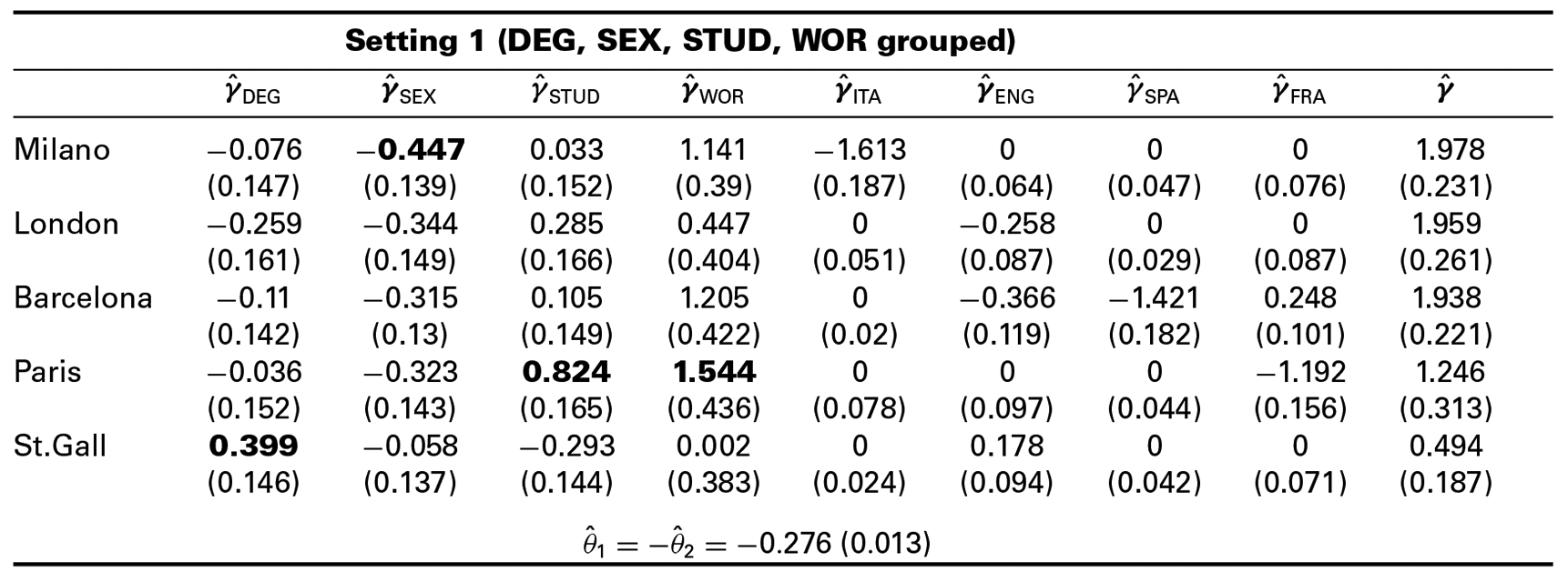
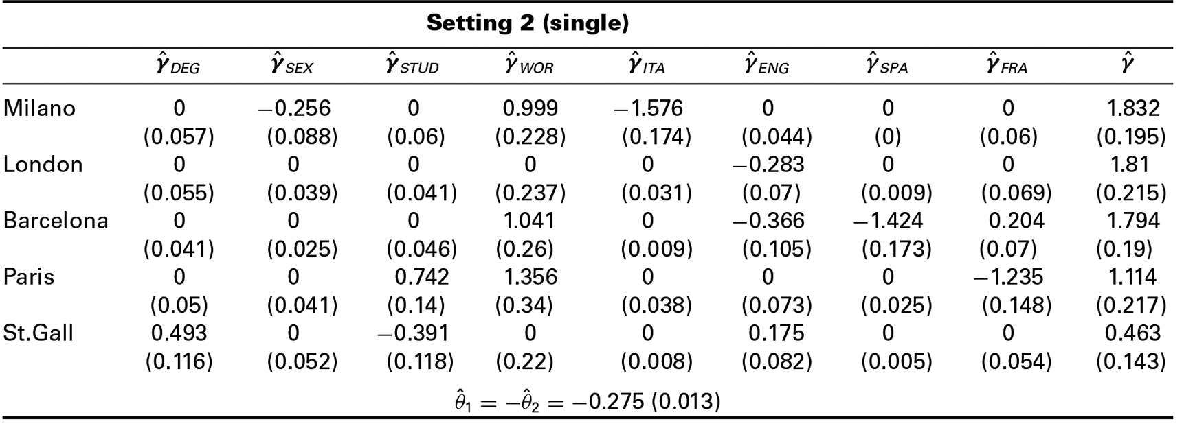
In the second setting, we use $V_{single} = {STUD, WOR, DEG, SEX, ENG, FRA, SPA, ITA}$ and $V_{grouped} = \emptyset$ . Thus, for each subject-specific covariate only the associated subject–object interactions are considered. For both settings, we apply the BTLboost algorithm to the cumulative BTL model using the AIC and BIC as stopping criteria. The estimated parameters after a final refitting step with bootstrapped standard errors can be found in Table 4 and Table 5. Because the BIC performed better in the simulation study, both tables show only the estimated parameters when using the BIC as stopping criterion. The optimal number of iterations when using the BIC was 34 in the first setting and 30 in the second setting.

Table 4

Estimates for selected subject–object interaction and object parameters after a final refitting step for Setting 1. The figures in brackets reflect standard error estimates based on $1000$ bootstrapped samples.

Setting 1 (DEG, SEX, STUD, WOR grouped)
	${\hat{γ}}_{DEG}$	${\hat{γ}}_{SEX}$	${\hat{γ}}_{STUD}$	${\hat{γ}}_{WOR}$	${\hat{γ}}_{ITA}$	${\hat{γ}}_{ENG}$	${\hat{γ}}_{SPA}$	${\hat{γ}}_{FRA}$	$\hat{γ}$
Milano	$-$ 0.076	$-$ 0.447	0.033	1.141	$-$ 1.613	0	0	0	1.978
	(0.147)	(0.139)	(0.152)	(0.39)	(0.187)	(0.064)	(0.047)	(0.076)	(0.231)
London	$-$ 0.259	$-$ 0.344	0.285	0.447	0	$-$ 0.258	0	0	1.959
	(0.161)	(0.149)	(0.166)	(0.404)	(0.051)	(0.087)	(0.029)	(0.087)	(0.261)
Barcelona	$-$ 0.11	$-$ 0.315	0.105	1.205	0	$-$ 0.366	$-$ 1.421	0.248	1.938
	(0.142)	(0.13)	(0.149)	(0.422)	(0.02)	(0.119)	(0.182)	(0.101)	(0.221)
Paris	$-$ 0.036	$-$ 0.323	0.824	1.544	0	0	0	$-$ 1.192	1.246
	(0.152)	(0.143)	(0.165)	(0.436)	(0.078)	(0.097)	(0.044)	(0.156)	(0.313)
St.Gall	0.399	$-$ 0.058	$-$ 0.293	0.002	0	0.178	0	0	0.494
	(0.146)	(0.137)	(0.144)	(0.383)	(0.024)	(0.094)	(0.042)	(0.071)	(0.187)
${\hat{θ}}_{1} = - {\hat{θ}}_{2} = - 0.276 (0.013)$

Source: Authors' computation.

Table 5

Estimates for selected subject–object interactions and object parameters after a final refitting step for Setting 2. The figures in brackets reflect standard error estimates based on $1000$ bootstrapped samples.

Setting 2 (single)
	${\hat{γ}}_{DEG}$	${\hat{γ}}_{SEX}$	${\hat{γ}}_{STUD}$	${\hat{γ}}_{WOR}$	${\hat{γ}}_{ITA}$	${\hat{γ}}_{ENG}$	${\hat{γ}}_{SPA}$	${\hat{γ}}_{FRA}$	$\hat{γ}$
Milano	0	$-$ 0.256	0	0.999	$-$ 1.576	0	0	0	\hskip 3.6pt1.832
	(0.057)	(0.088)	(0.06)	(0.228)	(0.174)	(0.044)	(0)	(0.06)	(0.195)
London	0	0	0	0	0	$-$ 0.283	0	0	\hskip 3.6pt1.81
	(0.055)	(0.039)	(0.041)	(0.237)	(0.031)	(0.07)	(0.009)	(0.069)	(0.215)
Barcelona	0	0	0	1.041	0	$-$ 0.366	$-$ 1.424	0.204	\hskip 3.6pt1.794
	(0.041)	(0.025)	(0.046)	(0.26)	(0.009)	(0.105)	(0.173)	(0.07)	(0.19)
Paris	0	0	0.742	1.356	0	0	0	$-$ 1.235	\hskip 2.8pt1.114
	(0.05)	(0.041)	(0.14)	(0.34)	(0.038)	(0.073)	(0.025)	(0.148)	(0.217)
St.Gall	0.493	0	$-$ 0.391	0	0	0.175	0	0	\hskip 3.4pt0.463
	(0.116)	(0.052)	(0.118)	(0.22)	(0.008)	(0.082)	(0.005)	(0.054)	(0.143)
${\hat{θ}}_{1} = - {\hat{θ}}_{2} = - 0.275 (0.013)$

Source: Authors' computation.

The results show that the ranking of objects (here universities), which is based on ordering the estimates for $\hat{γ}$ , is the same for both settings. Milan has the greatest estimate (e.g., ${\hat{γ}}_{Milan} = 1.978$ from Table 4) and thus the most preferred university is Milan, followed by London, Barcelona, Paris, St.Gall and the reference university Stockholm, for which $γ_{Stockholm} = 0$ . However, the ranking changes for different values of the subject-specific covariates. For example, if we consider students who are employed full-time while studying ( $WOR = 1$ ), the ranking is based on $\hat{γ} + {\hat{γ}}_{WOR}$ yielding a different university ranking for those students. The estimates ${\hat{γ}}_{London, ENG}, {\hat{γ}}_{Paris, FRA}, {\hat{γ}}_{Milan, ITA}$ and ${\hat{γ}}_{Barcelona, SPA}$ are all negative valued, and therefore they indicate that students with poor knowledge of English, French, Italian and Spanish have a lower tendency to prefer the universities in London, Paris, Milan and Barcelona, respectively. The main difference between Setting 1 and Setting 2 is that the subject–object interactions associated with the subject-specific covariates STUD, WOR, DEG and SEX were selected simultaneously in Setting 1 and separately in Setting 2. Nevertheless, all subject–object interactions that are highlighted in boldface in Table 4 were also identified in Setting 2. These subject–object interactions are the ones with the largest absolute value within the associated subject-specific parameter. Thus, the model from Setting 2 was able to identify the subject–object interactions from Setting 1 with the strongest effect.

7 Concluding remarks

Boosting is a technique that addresses the estimation problems in high-dimensional settings and provides variable selection when using component-wise boosting. In this article, we proposed a new estimation procedure for ordinal BTL models based on this technique. The simulation results showed that the method performs well concerning the identification of influential covariates. In the application section, the selected subject–object interactions are similar to those from the final model of Dittrich et. al. (1998), although they used a different model and a variable selection approach based on forward selection and backward elimination. In the algorithm proposed here, the variable selection is carried out during the fitting process. Thus, it can also be applied in cases where the maximum likelihood estimate does not exist, for example, when the data contains more subject-specific covariates than observations.

The model estimation for ordinal BTL models is computed with the ordBTL package (Casalicchio, 2013), which is implemented in the statistical software R (R Core Team, 2013). The package is able to fit models with any number of response categories and implements the BTLboost algorithm. The data used in Section 6 is also available in the package. Other packages for model estimation, which can handle responses up to 3 categories but have no built-in variable selection procedure, are prefmod (Hatzinger and Dittrich, 2012) and BradleyTerry2 (Turner and Firth, 2012).

8 Appendix A: Matrix representation

The representation used here is that of a multivariate generalized linear model, which has, in terms of paired comparisons, the following basic form

g (π^{(r, s), i}) = η^{(r, s), i} = X^{(r, s), i} β,

(A.1)

where

g

is a

(K - 1)

-dimensional link function,

β

is the vector of coefficients,

π^{(r, s), i} = {(π_{1}^{(r, s), i}, \dots, π_{K}^{(r, s), i})}^{⊤}

is the vector of response probabilities,

η^{(r, s), i} = {(η_{1}^{(r, s), i}, \dots, η_{K - 1}^{(r, s), i})}^{⊤}

is the subject-specific linear predictor, and

X^{(r, s), i}

is the design matrix for the pair

(r, s)

and subject

i

. If the design matrix and the link function

g

is specified, the Fisher scoring algorithm for multivariate maximum likelihood estimation can be used to obtain the parameter estimates (see Fahrmeir and Tutz, 2001; Tutz, 2012).

Before describing the design matrix in more detail, we first let $θ^{⊤} = (θ_{1}, \dots, θ_{q})$ , with $q = ⌊\frac{K - 1}{2}⌋$ , denote a vector containing all threshold parameters that have to be estimated and ${\tilde{θ}}^{⊤} = (θ_{1}, \dots, θ_{K - 1})$ denote a vector containing all threshold parameters in the model, including those that are restricted by the symmetry constraints from equations (2.3) and (2.4). For each pair $(r, s)$ and each subject $i$ , we define the matrix $Q^{(r, s), i}$ of dimension $(K - 1) \times q$ , such that

Q^{(r, s), i} θ_{} = \tilde{θ}

(A.2)

satisfies the symmetry constraints and ensures that the thresholds will be symmetric. Thus, the matrix can be seen as a so-called constraint matrix (for more details, see Yee, 2010).

To obtain the general structure of $Q^{(r, s), i}$ , we use the null vector $0_{q}^{⊤} = (0, \dots, 0)$ of length $q$ and the matrices

I_{q \times q} = (\begin{matrix} 1 & 0 & \dots & 0 \\ 0 & 1 & ⋱ & ⋮ \\ ⋮ & ⋱ & ⋱ & 0 \\ 0 & \dots & 0 & 1 \end{matrix}) and J_{q \times q} = (\begin{matrix} 0 & \dots & 0 & - 1 \\ ⋮ & ⋰ & - 1 & 0 \\ 0 & ⋰ & ⋰ & ⋮ \\ - 1 & 0 & \dots & 0 \end{matrix}) .

The matrix

Q^{(r, s), i}

satisfying equation (A.2) is a block matrix that has the same form for each pair

(r, s)

and each subject

i

, namely,

Q^{(r, s), i} = [\begin{matrix} I_{q \times q} \\ {0_{q}}^{⊤} \\ J_{q \times q} \end{matrix}] if K is even and Q^{(r, s), i} = [\begin{matrix} I_{q \times q} \\ J_{q \times q} \end{matrix}] if K is odd .

The subject-specific design matrix used in equation (A.1) is given by

X^{(r, s), i} = [Q^{(r, s), i}, \underset{\begin{matrix} X_{0}^{(r, s), i} \end{matrix}}{\underset{⏟}{1_{K - 1} \otimes {(x^{(r, s)})}^{⊤}}}, \underset{\begin{matrix} X_{1}^{(r, s), i} \end{matrix}}{\underset{⏟}{1_{K - 1} \otimes {(x_{1}^{(r, s), i})}^{⊤}}}, \dots, \underset{\begin{matrix} X_{P}^{(r, s), i} \end{matrix}}{\underset{⏟}{1_{K - 1} \otimes {(x_{P}^{(r, s), i})}^{⊤}}}],

where the vector

1_{K - 1} = {(1, \dots, 1)}^{⊤}

has the length

K - 1

. In a complete paired comparison experiment, we have

(\begin{matrix} M \\ 2 \end{matrix})

comparisons for each subject, where

(\begin{matrix} M \\ 2 \end{matrix}) = \frac{M!}{2! (M - 2)!}

denotes the binomial coefficient representing the number of all distinct pairs when comparing

M

different objects, namely,

(1, 2), (1, 3), \dots, (r, s), \dots, (M - 1, M), for all r < s .

The complete design matrix

X

contains information about all possible comparisons made by any subject and has therefore

I \cdot (\begin{matrix} M \\ 2 \end{matrix})

rows. It can be written as a block matrix of the form

X = [\begin{matrix} \begin{matrix} \begin{matrix} \begin{matrix} X^{(1, 2), 1} \\ ⋮ \end{matrix} \\ X^{(M - 1, M), 1} \end{matrix} \\ ⋮ \\ X^{(1, 2), I} \\ ⋮ \end{matrix} \\ X^{(M - 1, M), I} \end{matrix}] = [\begin{matrix} \begin{matrix} \begin{matrix} Q^{(1, 2), 1} \\ ⋮ \end{matrix} \\ Q^{(M - 1, M), 1} \\ ⋮ \end{matrix} \\ Q^{(1, 2), I} \\ ⋮ \\ \underset{Q}{\underset{︸}{Q^{(M - 1, M), 1}}} \end{matrix} \begin{matrix} \begin{matrix} \begin{matrix} X_{0}^{(1, 2), 1} \\ ⋮ \end{matrix} \\ X_{0}^{(M - 1, M), 1} \\ ⋮ \end{matrix} \\ Q_{0}^{(1, 2), I} \\ ⋮ \\ \underset{X_{0}}{\underset{︸}{Q_{0}^{(M - 1, M), 1}}} \end{matrix} \begin{matrix} \begin{matrix} \begin{matrix} X_{1}^{(1, 2), 1} \\ ⋮ \end{matrix} \\ X_{1}^{(M - 1, M)} \\ ⋮ \end{matrix} \\ X_{1}^{(1, 2), I} \\ ⋮ \\ \underset{X_{1}}{\underset{︸}{X_{1}^{(M - 1, M), 1}}} \end{matrix} \begin{matrix} \begin{matrix} \begin{matrix} \dots \end{matrix} \\ \dots \\ ⋮ \end{matrix} \\ \dots \\ \dots \end{matrix} \begin{matrix} \begin{matrix} \begin{matrix} X_{P}^{(1, 2), 1} \\ ⋮ \end{matrix} \\ X_{P}^{(M - 1, M), 1} \\ ⋮ \end{matrix} \\ X_{P}^{(1, 2), I} \\ ⋮ \\ \underset{X_{P}}{\underset{︸}{X_{P}^{(M - 1, M), 1}}} \end{matrix}],

where

Q

is the matrix for the thresholds

θ

X_{0}

is the matrix for the object parameters

γ

and

X_{1}, \dots, X_{P}

are matrices for the subject-specific parameters

γ_{1}, \dots, γ_{P}

The linear predictor $η = {({η^{(1, 2), 1}}^{⊤}, \dots, {η^{(M - 1, M), 1}}^{⊤}, \dots, {η^{(1, 2), I}}^{⊤}, \dots, {η^{(M - 1, M), I}}^{⊤})}^{⊤}$ contains all comparisons made by any subject and has the form $η = X β,$ with the vector $β = (θ^{⊤}, γ^{⊤}, γ_{1}^{⊤}, \dots, γ_{P}^{⊤})$ containing all parameters that have to be estimated, that is, all $q$ threshold parameters, all $M - 1$ object parameters and all $M - 1$ subject–object interaction parameters for each of the $P$ subject-specific covariates.

Footnotes

Acknowledgments

Financial support from LMUexcellent is gratefully acknowledged.

References

Agresti

(1992) Analysis of ordinal paired comparison data. Journal of the Royal Statistical Society. Series C (Applied Statistics) , 41, 287–97.

Böckenholt

(2001) Hierarchical modeling of paired comparison data. Psychological Methods , 6, 49.

Bradley

Terry

(1952) Rank analysis of incomplete block designs: I. The method of paired comparisons. Biometrika , 39, 324–45.

Bühlmann

(2006) Boosting for high-dimensional linear models. The Annals of Statistics , 34, 559–83.

Bühlmann

Hothorn

(2007a) Boosting algorithms: Regularization, prediction and model fitting. Statistical Science , 22, 477–505.

Bühlmann

Hothorn

(2007b) Rejoinder: Boosting algorithms: Regularization, prediction and model fitting. Statistical Science , 22, 516–22.

Bühlmann

(2003) Boosting with the L₂-loss: Regression and classification. Journal of the American Statistical Association , 98, 324–39.

Casalicchio

(2013) ordBTL: Modelling comparison data with ordinal response . R package version 0.8.

Davidson

(1970) On extending the Bradley-Terry model to accommodate ties in paired comparison experiments. Journal of the American Statistical Association , 65, 317–28.

10.

Dittrich

Hatzinger

Katzenbeisser

(1998) Modelling the effect of subject-specific covariates in paired comparison studies with an application to university rankings. Journal of the Royal Statistical Society: Series C (Applied Statistics) , 47, 511–25.

11.

Dittrich

Hatzinger

Katzenbeisser

(2004) A log-linear approach for modelling ordinal paired comparison data on motives to start a PhD programme. Statistical Modelling , 4, 181–93.

12.

Dittrich

Francis

Hatzinger

Katzenbeisser

(2007) A paired comparison approach for the analysis of sets of Likert-scale responses. Statistical Modelling , 7, 3–28.

13.

Fahrmeir

Tutz

(2001) Multivariate statistical modelling based on generalized linear models . New York: Springer.

14.

Francis

Dittrich

Hatzinger

Penn

(2002) Analysing partial ranks by using smoothed paired comparison methods: An investigation of value orientation in Europe. Journal of the Royal Statistical Society: Series C (Applied Statistics) , 51, 319–36.

15.

Freund

(1995) Boosting a weak learning algorithm by majority. Information and Computation , 121, 256–85.

16.

Freund

(1997) A decision-theoretic generalization of on-line learning and an application to boosting? Journal of Computer and System Sciences , 55, 119–39.

17.

Friedman

Hastie

Tibshirani

(2000) Special invited paper. Additive ogistic regression: A statistical view of boosting. The Annals of Statistics , 28, 337–74.

18.

Friedma

(2001) Greedy function approximation: A gradient boosting machine. The Annals of Statistics , 29, 1189–232.

19.

Hatzinger

Dittrich

(2012) prefmod: An R package for modeling preferences based on paired comparisons, rankings, or ratings. Journal of Statistical Software , 48, 1–31.

20.

Luce

(1959) Individual choice behavior a theoretical analysis . New York: Wiley.

21.

McCullagh

(1980) Regression models for ordinal data. Journal of the Royal Statistical Society. Series B (Methodological) , 42, 109–42.

22.

R Core Team (2013) R: A language and environment for statistical computing . R Foundation for Statistical Computing Vienna, Austria.

23.

Rao

Kupper

(1967) Ties in paired-comparison experiments: A generalization of the Bradley-Terry model. Journal of the American Statistical Association , 62, 194–204.

24.

Schapire

(1990) The strength of weak learnability. Machine Learning , 5, 197–227.

25.

Turner

Firth

(2012) Bradley-Terry models in R: The BradleyTerry2 package. Journal of Statistical Software , 48.

26.

Tutz

(1986) Bradley-Terry-Luce models with an ordered response. Journal of Mathematical Psychology , 30, 306–16.

27.

Tutz

(2012) Regression for categorical data . Cambridge University Press.

28.

Tutz

Binder

(2006) Generalized additive modeling with implicit variable selection by likelihood-based boosting. Biometrics , 62, 961–71.

29.

Yee

(2010) The VGAM package for categorical data analysis. Journal of Statistical Software , 32, 1–34.

30.

Zahid

Tutz

(2013) Proportional odds models with high-dimensional data structure. International Statistical Review , 81, 388–406.

Subject-specific Bradley–Terry–Luce models with implicit variable selection

Abstract

Keywords

1 Introduction

2 Paired comparison models

2.1 The binary BTL model

2.2.1 The cumulative model

4 Boosting

4.1 Basic concept of boosting

4.2 Boosting ordinal BTL models

4.3 Stopping criteria

5.1 Simulation set-up

Table 1 Influential subject–object interaction parameters.

8 Appendix A: Matrix representation

Footnotes

Acknowledgments

References

Table 1
Influential subject–object interaction parameters.