Nuclear penalized multinomial regression with an application to predicting at bat outcomes in baseball

Abstract

We propose the nuclear norm penalty as an alternative to the ridge penalty for regularized multinomial regression. This convex relaxation of reduced-rank multinomial regression has the advantage of leveraging underlying structure among the response categories to make better predictions. We apply our method, nuclear penalized multinomial regression (NPMR), to Major League Baseball play-by-play data to predict outcome probabilities based on batter–pitcher matchups. The interpretation of the results meshes well with subject-area expertise and also suggests a novel understanding of what differentiates players.

Keywords

multinomial regression Reduced-rank regression baseball nuclear norm proximal gradient descent

1 Introduction

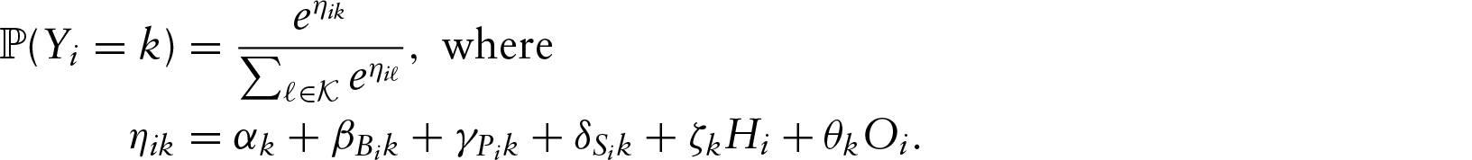
A baseball game comprises a sequence of matchups between one batter and one pitcher. Each matchup, or plate appearance (PA), results in one of several outcomes. Disregarding some obscure possibilities, we consider nine categories for PA outcomes: flyout (F), groundout (G), strikeout (K), base on balls (BB), hit by pitch (HBP), single (1B), double (2B), triple (3B) and home run (HR).

A problem which has received a prodigious amount of attention in sabermetric (the study of baseball statistics) literature is determining the value of each of the above outcomes, as it leads to scoring runs and winning games. But that is only half the battle. Much less work in this field focuses on an equally important problem: optimally estimating the probabilities with which each batter and pitcher will produce each PA outcome. Even for ‘advanced metrics’, this second task is usually done by taking simple empirical proportions, perhaps shrinking them towards a population mean using a Bayesian prior.

In statistics literature, on the other hand, many have developed shrinkage estimators for a set of probabilities with application to batting averages, starting with Stein's estimator (Efron and Morris, 1975). Since then, Bayesian approaches to this problem have been popular. Morris (1983) and Brown (2008) used empirical Bayes for estimating batting averages, which are binomial probabilities. We are interested in estimating multinomial probabilities, such as the nested Dirichlet model of Null (2009) and the hierarchical Bayesian model of Albert (2016). What all of the earlier works have in common is that they do not account for the ‘strength of schedule’ faced by each player: How skilled were his opponents?

The state-of-the-art approach, Deserved Run Average (Judge and BP Stats Team, 2015; DRA) is similar to the adjusted plus–minus model from basketball and the Rasch model used in psychometrics. The latter models the probability (on the logistic scale) that a student correctly answers an exam question as the difference between the student's skill and the difficulty of the question. DRA models players’ skills as random effects and also includes fixed effects like the identity of the ballpark where the PA took place. Each category of the response has its own binomial regression model. Taking HR as an example, each batter $B$ has a propensity $β_{B}^{HR}$ for hitting home runs, and each pitcher $P$ has a propensity $γ_{P}^{HR}$ for allowing home runs. Distilling the model to its elemental form, if $Y$ denotes the outcome of a PA between batter $B$ and pitcher $P$ ,

ℙ (Y = HR | B, P) = \frac{e^{α^{HR} + β_{B}^{HR} + γ_{P}^{HR}}}{1 + e^{α^{HR} + β_{B}^{HR} + γ_{P}^{HR}}} .

(Actually, in detail DRA uses the probit rather than the logit link function.)

One bothersome aspect of DRA is that the probability estimates do not sum to one; a natural solution is to use a single multinomial regression model instead of several independent binomial regression models. Making this adjustment would result in a model very similar to ridge multinomial regression (described in Section 3.3), and we will compare the results of our model with the results of ridge regression as a proxy for DRA. Ridge multinomial regression applied to this problem has about 8 000 parameters to estimate (one for each outcome for each player) on the basis of about 160 000 PAs in a season, bound together only by the restriction that probability estimates sum to one. One may seek to exploit the structure of the problem to obtain better estimates, as in ordinal regression. The categories have an ordering, from least to most valuable to the batting team:

K < G < F < BB < HBP < 1 B < 2 B < 3 B < HR,

with the ordering of the first three categories depending on the game situation. But the proportional odds model used for ordinal regression assumes that when one outcome is more likely to occur, the outcomes close to it in the ordering are also more likely to occur. That assumption is woefully off base in this setting because as we show in the following, players who hit a lot of home runs tend to strike out often, and they tend not to hit many triples. The proportional odds model is better suited for response variables on the Likert scale (Likert, 1932), for example.

Figure 1:

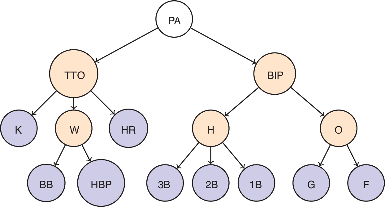
Illustration of the hierarchical structure among the PA outcome categories, adapted from Baumer and Zimbalist (2014). Dark terminal nodes correspond to the nine outcome categories in the data. Light internal nodes have the following meaning: TTO, three true outcomes; BIP, balls in play; W, walks; H, hits; O, outs. Outcomes close to each other (in terms of number of edges separating them) tend to occur in similar circumstances

The actual relationships among the outcome categories are more similar to the hierarchical structure illustrated by Figure 1. The outcomes fall into two categories: balls in play (BIP) and the ‘three true outcomes’ (TTO). The TTO, as they have become traditionally known in sabermetric literature, include home runs, strikeouts and walks (which itself includes BB and HBP). The distinction between BIP and TTO is important because the former category involves all eight position players in the field on defence, whereas the latter category involves only the batter and the pitcher. Figure 1 has been designed (roughly) by baseball experts so that terminal nodes close to each other (by the number of edges separating them) are likely to co-occur. Players who hit a lot of home runs tend to strike out a lot, and the outcomes K and HR are only two edges away from each other. Hence, the graph reveals something of the underlying structure in the outcome categories.

Figure 2:

Biplots of the principal component analyses of player outcome matrices, separate for batters and pitchers. The dots represent players and the arrows (corresponding to the top and right axes) show the loadings for the first two principal components on each of the outcomes. We exclude outcomes for which the loadings of both of the first two principal components are sufficiently small

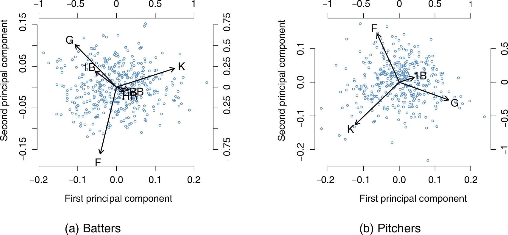
This structure is further evidenced by principal component (PC) analysis of the player–outcome matrix, illustrated in Figure 2 and Table 1. The player–outcome matrix has a row for each player giving the proportion of PAs which have resulted in each of the nine outcomes in the dataset. For batters, the PC which describes most of the variance in observed outcome probabilities has negative loadings on all of the BIP outcomes and positive loadings on all of the TTO outcomes. For both batters and pitchers, the percentage of variance explained after two PCs drops off precipitously.

Table 1:

Visualization of principal component analysis of player–outcome matrices, separate for batters and for pitchers. The visualization shows the loadings for each PC, along with a highlighted bar plot corresponding to the percentage of variance explained by each PC, which is also printed in the row below the matrix of PC loadings

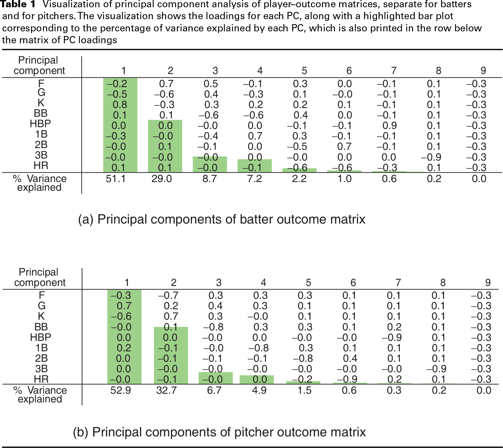
PC analysis is useful for illustrating the relationships between the outcome categories. For example, Table 1(a) suggests that batters who tend to hit singles (1B) more than average also tend to ground out (G) more than average. So an estimator of a batter's groundout rate could benefit from taking into account the batter's single rate, and vice versa. This is an example of the type of structure in outcome categories that motivates our proposal, which aims to leverage this structure to obtain better regression coefficient estimates in multinomial regression.

In Section 2, we review reduced-rank multinomial regression, a first attempt at leveraging this structure. We improve on this in Section 3 by proposing nuclear penalized multinomial regression (NPMR), a convex relaxation of the reduced-rank problem. We compare our method with ridge regression in a simulation study in Section 4. In Section 5, we apply our method and interpret the results on the baseball data, as well as another application. The manuscript concludes with a discussion in Section 6.

2 Multinomial logistic regression and reduced rank

Suppose that we observe data $x_{i} \in ℝ^{p}$ and $Y_{i} \in {1, . . ., K}$ for $i = 1, . . ., n$ . We use $X$ to denote the matrix with rows $x_{i}$ , specifically $X = (x_{1}, . . ., x_{n})^{T}$ . The multinomial logistic regression model assumes that the $Y_{i}$ are conditional on $X$ , independent and that for $k = 1, . . ., K :$

ℙ (Y_{i} = k | x_{i}) = \frac{e^{α_{k} + x_{i}^{T} β_{k}}}{\sum_{ℓ = 1}^{K} e^{α_{ℓ} + x_{i}^{T} β_{ℓ}}},

(2.1)

where

α_{k} \in ℝ

and

β_{k} \in ℝ^{p}

are fixed, unknown parameters. The model (2.1) is not identifiable because an equal increase in the same element of each of the

β_{k}

(or in each of the

α_{k}

) does not the change the estimated probabilities. That is, for each choice of parameter values, there is an infinite set of choices which have the same likelihood as the original choice, for any observed data. This problem may readily be resolved by adopting the restriction for some

k_{0} \in {1, . . ., K}

that

α_{k_{0}} = 0

and

β_{k_{0}} = 0_{p}

. However, depending on the method used to fit the model, this identifiability issue may not interfere with the existence of a unique solution; in such a case, we do not adopt this restriction. For example, fitting the model with ridge regression would involve minimizing the sum of the negative log-likelihood and the sum of squares of the regression coefficients. Adding this strictly convex function to the objective leads to a unique solution. See the appendix for a detailed discussion.

In contrast with logistic regression, multinomial regression involves estimating not a vector but a matrix of regression coefficients: one for each independent variable, for each class. We denote this matrix by $B = (β_{1}, . . ., β_{K})$ . Motivated by the PC analysis from Section 1, instead of learning a coefficient vector for each class, we might do better by learning a coefficient vector for each of a smaller number $r$ of latent variables, each having a loading on the classes. For $r = 1$ , this is the stereotype model originally proposed by Anderson (1984), who observed its applicability to multinomial regression problems with structure between the response categories, including ordinal structure. Greenland (1994) argued for the stereotype model as an alternative in medical applications to the standard techniques for ordinal categorical regression: the cumulative-odds and continuation-ratio models.

Yee and Hastie (2003) generalized the model to reduced-rank vector generalized linear models. In detail, the reduced-rank multinomial logistic model (RR-MLM) fits (2.1) by solving, for some $r \in {1, . . ., K - 1}$ , the optimization problem:

\begin{array}{l} \underset{α \in ℝ^{K}, B \in ℝ^{p \times K}}{minimize} - \sum_{i = 1}^{n} \log (\sum_{k = 1}^{K} \frac{e^{α_{k} + x_{i}^{T} β_{k}}}{\sum_{l = 1}^{K} e^{α_{l} + x_{i}^{T} β_{l}}} 𝕀_{{Y_{i} = k}}) \\ subject to rank (B) \leq r, α_{1} = 0, β_{1} = 0_{p} . \end{array}

(2.2)

If rank

(B) < r

, then there exist

A \in ℝ^{p \times r}

C \in ℝ^{K \times r}

such that

B = A C^{T}

. Under this factorization, the

r

columns of

C

can be interpreted as defining latent outcome variables, each with a loading on each of the

K

outcome classes. The

r

columns of

A

give regression coefficient vectors for these latent outcome variables rather than the outcome classes.

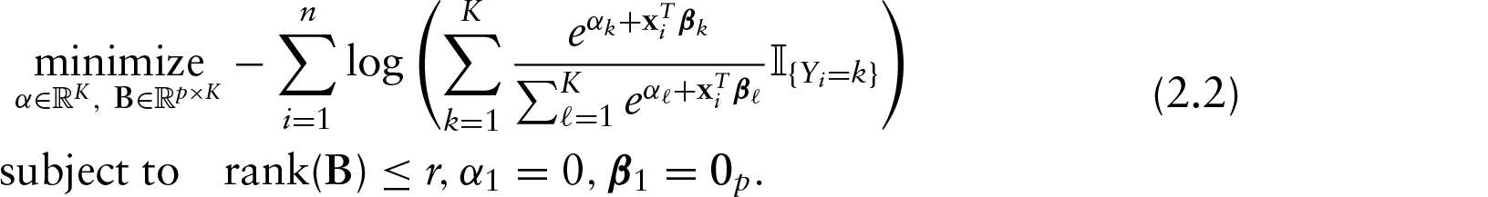
The optimization problem (2.2) is not convex because rank $(\cdot)$ is not a convex function. Yee (2010) implemented an alternating algorithm to solve it in the R (R Core Team, 2016) package VGAM. However, this algorithm is too slow for feasible application to datasets as large as the one motivating Section 1. See Section 5.1 for a detailed description of the dataset.

3 Nuclear penalized multinomial regression

Because of the computational difficulty of solving (2.2), we propose replacing the rank restriction with a restriction on the nuclear norm $| | \cdot | |_{*}$ (defined in the following) of the regression coefficient matrix. For some $ρ > 0$ , this convex optimization problem is:

\begin{array}{l} \underset{α \in ℝ^{K}, B \in ℝ^{p \times K}}{minimize} - \sum_{i = 1}^{n} \log (\sum_{k = 1}^{K} \frac{e^{α_{k} + x_{i}^{T} β_{k}}}{\sum_{ℓ = 1}^{K} e^{α_{ℓ} + x_{i}^{T} β_{ℓ}}} 𝕀_{{Y_{i} = k}}) \\ subject to {‖ B ‖}_{*} \leq ρ . \end{array}

(3.1)

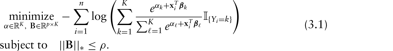
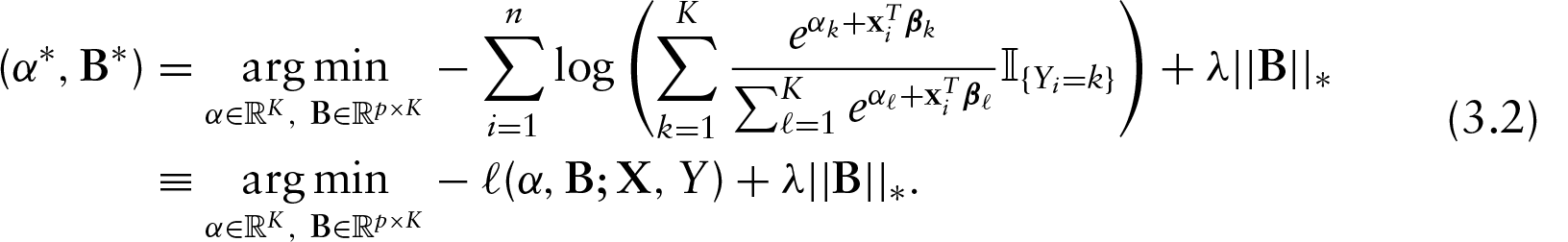
We prefer to frame the problem in its equivalent Lagrangian form: For some $λ > 0$ ,

\begin{array}{l} (α^{*}, B^{*}) = \underset{α \in ℝ^{K}, B \in ℝ^{p \times K}}{arg min} - \sum_{i = 1}^{n} \log (\sum_{k = 1}^{K} \frac{e^{α_{k} + x_{i}^{T} β_{k}}}{\sum_{ℓ = 1}^{K} e^{α_{ℓ} + x_{i}^{T} β_{ℓ}}} 𝕀_{{Y_{i} = k}}) + λ {‖ B ‖}_{*} \\ \equiv \underset{α \in ℝ^{K}, B \in ℝ^{p \times K}}{arg min} - ℓ (α, B; X, Y) + λ {‖ B ‖}_{*} \end{array}

(3.2)

This optimization problem (3.2) is what we call NPMR. We use

ℓ (α, B; X, Y)

to denote the log-likelihood of the regression coefficients

α

and B, given the data

X

and

Y

. The nuclear norm of a matrix is defined as the sum of its singular values, that is, the

ℓ_{1}

-norm of its vector of singular values. Explicitly, consider the singular value decomposition of B given by

Σ V^{T}

, with

U \in ℝ^{p \times p}

and

V \in ℝ^{K \times K}

orthogonal and

Σ \in ℝ^{p \times K}

having values

σ_{1}, . . ., σ_{\min {p, K}}

along the main diagonal and zeros elsewhere. Then

{‖ B ‖}_{*} = \sum_{d = 1}^{\min {p, K}} σ_{d} .

In the same way that the lasso induces sparsity of the estimated coefficients in a regression, solving (3.2) drives some of the singular values to exactly zero. Because the number of nonzero singular values is the rank of a matrix, the result is that the estimated coefficient matrix

B^{*}

tends to have less than full rank. Thus, (3.2) is a convex relaxation of the reduced-rank multinomial logistic regression problem, in much the same way as the lasso is a convex relaxation of the best subset regression (Tibshirani, 1996). The convexity of (3.2) makes it easier to solve than (2.2), and we discuss algorithms for solving it in Sections 3.1 and 3.2. In practice, we recommend using standard cross-validation (CV) techniques for selecting the regularization parameter

λ

, which controls the rank of the solution. For CV loss, we use multinomial deviance; other choices are valid. Throughout this manuscript we use ten fold CV.

Consider the singular value decomposition $U^{*} Σ^{*} V^{* T}$ of the $p \times K$ estimated coefficient matrix $B^{*}$ . Each column of the $K \times K$ orthogonal matrix $V^{*}$ represents a latent variable as a linear combination of the $K$ outcome categories. Meanwhile, each row of $U^{*} Σ^{*}$ specifies for each predictor variable a coefficient for each latent variable, rather than for each outcome category. By estimating some of the singular values of $B^{*}$ (the entries of the diagonal $p \times K$ matrix $Σ^{*}$ ) to be zero, we reduce the number of coefficients to be estimated for each predictor variable from (a) one for each of $K$ outcome categories; to (b) one for each of some smaller number of latent variables. These latent variables learned by the model express relationships between the outcomes because two categories for which a latent variable has both large positive coefficients are both likely to occur for large values of that latent variable. Similarly, if a latent variable has a large positive coefficient for one category and a large negative coefficient for another, those two categories oppose each other diametrically with respect to that latent variable.

3.1 Proximal gradient descent

NPMR relies on solving (3.2). The objective is convex but non-differentiable where any singular values of B are zero, so we cannot use gradient descent. Generally, when minimizing a function $f : ℝ^{d} \to ℝ$ of a vector $x \in ℝ^{d}$ , the gradient descent update of step size $s$ takes the form

x^{(t + 1)} = x^{(t)} - s \nabla f (x^{(t)}),

or equivalently (Hastie et al., 2015),

x^{(t + 1)} = \underset{x \in ℝ^{d}}{arg min} ł {f (x^{(t)}) + ⟨ \nabla f (x^{(t)}), x - x^{(t)} ⟩ + \frac{1}{2 s} | | x - x^{(t)} | |_{2}^{2}} .

Still, if

f

is non-differentiable, as it is in (3.2), then

\nabla f

is undefined. However, if

f

is the sum of two convex functions

g

and

h

, with

g

differentiable, we can instead apply the generalized gradient update step (Hastie et al., 2015):

x^{(t + 1)} = \underset{x \in ℝ^{d}}{arg min} ł {g (x^{(t)}) + ⟨ \nabla g (x^{(t)}), x - x^{(t)} ⟩ + \frac{1}{2 s} | | x - x^{(t)} | |_{2}^{2} + h (x)} .

(3.3)

Repeatedly applying this update is known as proximal gradient descent (PGD). In (3.2), we have

x = (α, B)

g = - ℓ

and

h = | | \cdot | |_{*}

. So the PGD update step is:

\begin{matrix} (α^{(t + 1)}, B^{(t + 1)}) = & \arg \min_{α, B} {- ℓ (α^{(t)}, . B^{(t)}; X, Y) \\ + ⟨ - X^{T} (Y - P^{(t)}), B - B^{(t)} ⟩ + ⟨ - 1_{n}^{T} (Y - P^{(t)}), α - α^{(t)} ⟩ \\ + \frac{1}{2 s} | | B - B^{(t)} | |_{F}^{2} + \frac{1}{2 s} | | α - α^{(t)} | |_{2}^{2} + λ | | B | |_{*}}, \end{matrix}

where

Y \in {0, 1}^{n \times K}

is the matrix containing the response variable and

P \in (0, 1)^{n \times K}

is the matrix containing the fitted values. That is, for

i = 1, . . ., n

and

k = 1, . . ., K

{Y}_{i k} = 𝕀_{{Y_{i = k}}}, and {P}_{i k} = \frac{e^{α_{k} + x_{i}^{T} β_{k}}}{\sum_{ℓ = 1}^{k} e^{α_{ℓ} + x_{i}^{T} β_{ℓ}}} .

(3.4)

The squared Frobenius norm

| | \cdot | |_{F}^{2}

is the sum of the squares of the entries of a matrix.

The problem is separable in $α$ and B:

\begin{matrix} \begin{matrix} α^{(t + 1)} & = \arg \min_{α} {⟨ - 1_{n}^{T} (Y - P^{(t)}), α - α^{(t)} ⟩ + \frac{1}{2 s} | | α - α^{(t)} | |_{2}^{2}} \\ = α^{(t)} + s 1_{n}^{T} (Y - P^{(t)}), and \end{matrix} \end{matrix}

(3.5)

\begin{matrix} \begin{matrix} B^{(t + 1)} & = \arg \min_{B} {⟨ - X^{T} (Y - P^{(t)}), B - B^{(t)} ⟩ + \frac{1}{2 s} | | B - B^{(t)} | |_{F}^{2} + λ | | B | |_{*}} \\ = S_{s λ}^{*} (B^{(t)} + s X^{T} (Y - P^{(t)})), \end{matrix} \end{matrix}

(3.6)

where

S_{s λ}^{*} : ℝ^{p \times K} \to ℝ^{p \times K}

is the soft-thresholding operator on the singular values of a matrix. Explicitly, if a matrix

M \in ℝ^{p \times K}

has singular value decomposition

U Σ V^{T}

, then

S_{s λ}^{*} (M) = U S_{s λ} (Σ) V^{T}

, where

{S_{s λ} (Σ)}_{jk} = sign (Σ_{jk}) \max {| Σ_{jk} | - s λ, 0} .

S_{s λ}^{*}

is called the proximal operator of the nuclear norm, and in general solving (3.3) involves the proximal operator of

h

, hence the name PGD.

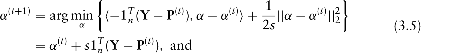
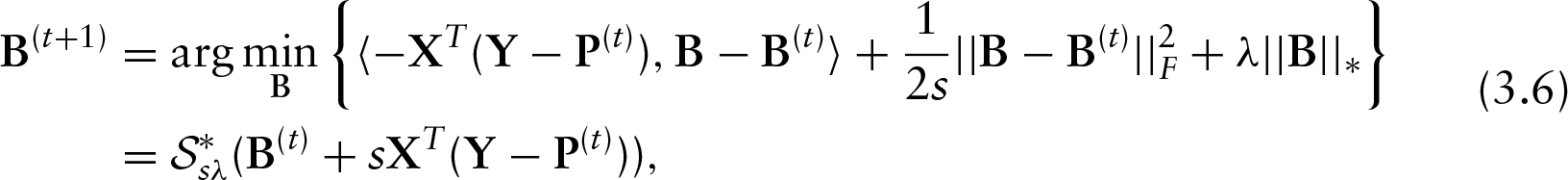
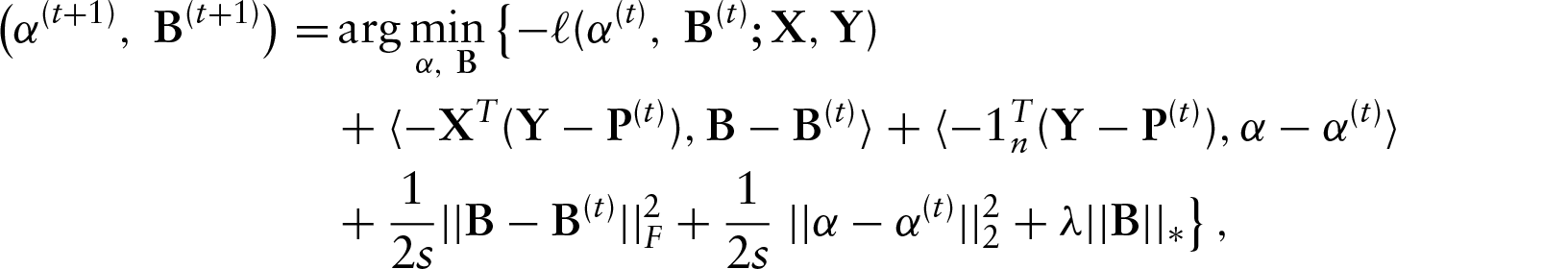
So to solve (3.2), initialize $α$ and B, and iteratively apply the updates (3.5) and (3.6). Due to Nesterov (2007), this procedure converges with step size $s \in (0, 1 / L)$ if the log-likelihood $ℓ$ is continuously differentiable and has Lipschitz gradient with Lipschitz constant $L$ . The appendix includes a proof that the gradient of $ℓ$ is Lipschitz with constant $L = \sqrt{K} | | X | |_{F}^{2}$ , but in practice we recommend starting with step size $s = 0.1$ and halving the step size if any PGD step would result in an increase of the objective function (3.2).

3.2 Accelerated PGD

In practice, we find that it helps to speed things up considerably to use an accelerated PGD method, also due to Nesterov (2007). Specifically, we iteratively apply the following updates:

$α^{(t + 1)} = α^{(t)} + s 1_{n}^{T} (Y - P^{(t)})$

$A^{(t + 1)} = B^{(t)} + \frac{t}{t + 3} (B^{(t)} - B^{(t - 1)})$

$P^{(t + 1)} = P (α^{(t + 1)}, A^{(t + 1)})$

$B^{(t + 1)} = S_{s λ}^{*} (A^{(t + 1)} + s X^{T} (Y - P^{(t + 1)}))$

The function $P (\cdot)$ in Step 3 returns the matrix of fitted probabilities based on the regression coefficients as described in (3.4). Step 2 is the key to the acceleration because it uses the ‘momentum’ in B to push it further in the same direction it is heading. We strongly recommend using this accelerated version of PGD, and our implementation of NPMR is available on the Comprehensive R Archive Network as the R package npmr.

3.3 Related work

Tutz and Gertheiss (2016) provide a systematic review of regularized regression for categorical data. NPMR is a novel method in this category and would fit well in their section on categorical response variables. The authors describe penalties for variable selection multinomial logistic regression and in ordinal regression. None of these methods induces low rank in the solution, as NPMR does. The idea of using a nuclear norm penalty as a convex relaxation to reduced-rank regression has previously been proposed in the Gaussian regression setting (Chen et al., 2013), but we are not aware of any attempt to do so in the multinomial setting.

The nearest competitor to NPMR that can feasibly be applied to the baseball matchup dataset is multinomial ridge regression, which penalizes the squared Frobenius norm (the sum of the squares of the entries) of the coefficient matrix, instead of the nuclear norm. In detail, ridge regression estimates the regression coefficients by solving the optimization problem

(α^{*}, B^{*}) = \underset{α \in ℝ^{K}, B \in ℝ^{p \times K}}{\arg \min} - ℓ (α^{(t)}, B^{(t)}; X, Y) + λ {‖ B ‖}_{F}^{2} .

(3.7)

This model is very similar to the state of the art in public sabermetric literature for evaluating pitchers on the basis of outcomes while simultaneously controlling for sample size, opponent strength and ballpark effects (Judge and BP Stats Team, 2015). Software is available to solve this problem very quickly in the R package glmnet (Friedman et al., 2010). This is the standard approach used for regularized multinomial regression problems, so we use it as the benchmark against which to compare the performance of NPMR in Sections 4 and 5.

4 Simulation study

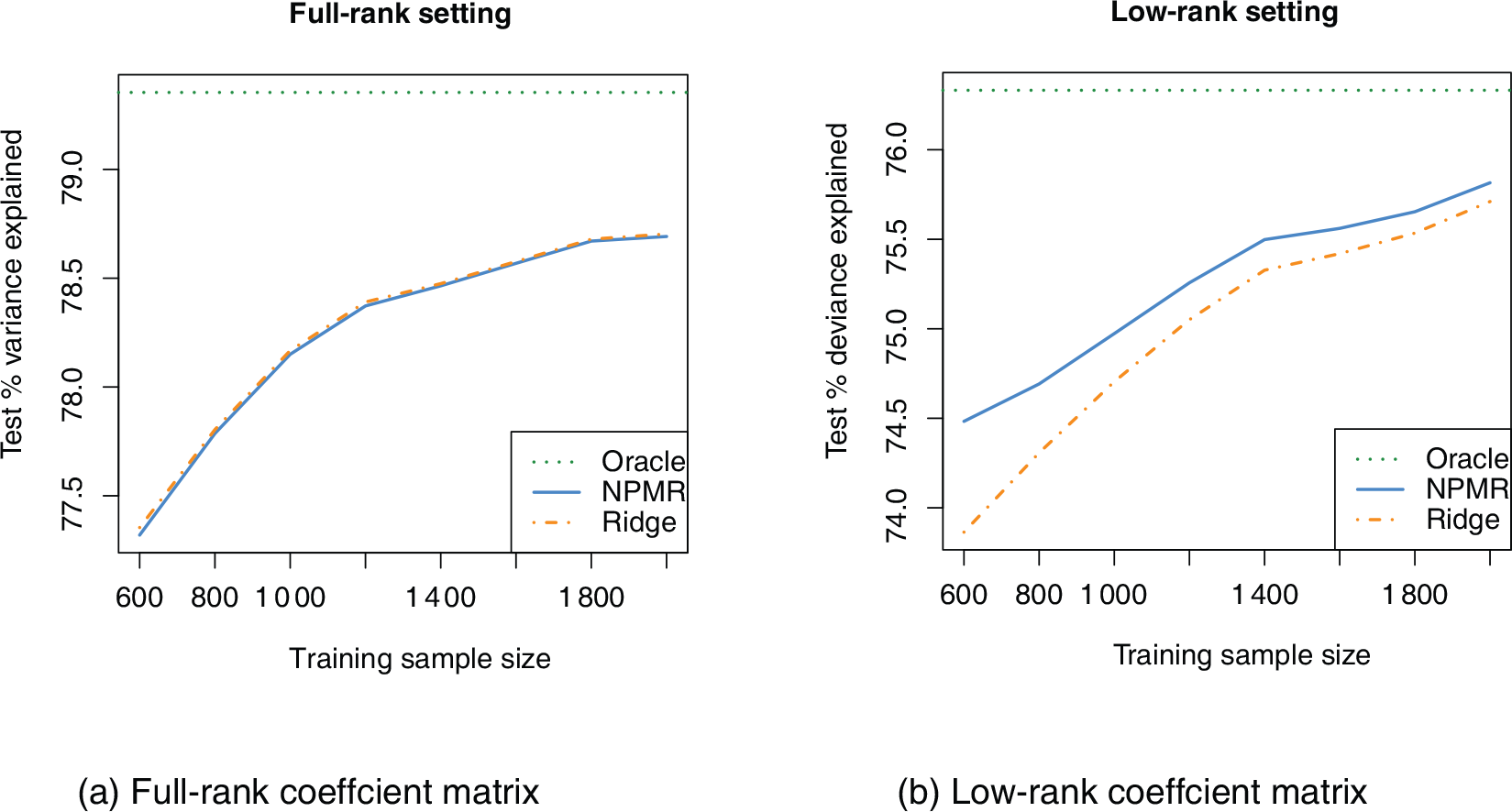
In this section, we present the results of two different simulations, one using a full-rank coefficient matrix and the other using a low-rank coefficient matrix. In both settings, we vary the training sample size $n$ from 600 to 2 000, and we fix the number of predictor variables to be 12 and the number of levels of the response variable to be 8. Given design matrix $X \in ℝ^{n \times 12}$ and coefficient matrix $B \in ℝ^{12 \times 8}$ , we simulate the response according to the multinomial regression model. Explicity, for $i = 1, . . ., n$ and $k = 1, . . ., 8$ ,

ℙ (Y_{i} = k) = \frac{e^{X β_{k}}}{\sum_{ℓ = 1}^{8} e^{X β_{ℓ}}} .

For both simulations, the entries of

X

are i.i.d. standard normal:

x_{i} \overset{i .i .d .}{\sim} Normal (0_{12}, I_{12})

for

i = 1, . . ., n

. However, the simulations differ in the generation of the coefficient matrix B. In the full-rank setting, the entries of B follow an i.i.d. standard normal distribution: For

k = 1, . . ., 8

β_{k} \overset{i .i .d .}{\sim} Normal (0_{12}, I_{12}) .

(4.1)

Figure 3:

Simulation results. We plot the percentage of deviance explained in a test set against training sample size. The oracle prediction is based on the known class probabilities from which the test class was drawn. In (a), the full-rank setting, ridge regression outperforms NPMR by a slim margin. In (b), the low-rank setting, NPMR wins, especially for smaller sample sizes

In the low-rank setting, we first simulate two intermediary matrices $A \in ℝ^{12 \times 2}$ and $C \in ℝ^{8 \times 2}$ with i.i.d. standard normal entries, and we then define $B = A C^{T}$ so that the rank of B is 2. In each simulation, we fit ridge regression and NPMR to the training sample of size $n$ and estimate the out-of-sample error by simulating 10 000 test observations, comparing the model's predictions on those test observations with the simulated response. The results of 3 500 simulations in each setting, for each training sample size $n$ , are presented in Figure 3.

In these simulations and throughout this manuscript, we evaluate the methods using percentage of deviance explained in the test set. Multinomial deviance is twice the negative log of the probability predicted for the class observed. The null deviance corresponds to using the overall frequency of each class in the training set as the predicted probability for that class. The percentage of deviance explained is the difference between the null deviance and the deviance of the method's predictions, divided by the null deviance.

In the full-rank setting, we expect ridge regression to out perform NPMR because ridge regression shrinks all coefficient estimates towards zero, which is the mean of the generating distribution for the coefficients in the simulation. If this were a Gaussian regression problem instead of a multinomial regression problem, then the ridge regression coefficient estimates would correspond (Hastie et al., 2009) to the posterior mean estimate under a Bayesian prior of (4.1). In fact, ridge regression does beat NPMR in this simulation (for all training sample sizes $n$ ), but NPMR's performance is surprisingly close to that of ridge regression.

The low-rank setting is one in which NPMR should have better test performance than does ridge regression. NPMR bets on sparsity in the singular values of the coefficient matrix, and in this setting the bet pays off. The simulation results verify that this intuition is correct. NPMR beats ridge regression for all training sample sizes $n$ , but especially for smaller sample sizes. By betting (correctly in this case) on the coefficient matrix having less than full rank, NPMR learns more accurate estimates of the coefficient matrix. As the training sample size increases, learning the coefficient matrix becomes easier, and the performance gap between the two methods shrinks but remains evident.

In summary, this simulation demonstrates that each of NPMR and ridge regression is superior in a simulation tailored to its strengths, confirming our intuition. Furthermore, in a simulation constructed in favour of ridge regression, NPMR performs nearly as well. Meanwhile, NPMR leads to more significant gains over ridge regression in the low-rank setting. In this simulation and in the applications to follow, the number of response categories is more than just a few. This is intentional; for a small number of classes, for example, $K = 3 or 4$ , then ridge regression would estimate a low-rank regression coefficient matrix itself, as the rank can be no larger than the number of columns.

5 Results

5.1 Implementation details

The 2015 MLB play-by-play dataset from Retrosheet includes an entry for every PA during the six-month regular season. For the purposes of fitting NPMR to predict the outcomes of PAs, the following relevant variables are recorded for the $i^{th}$ PA: the identity ( $B_{i}$ ) of the batter; the identity ( $P_{i}$ ) of the pitcher; the identity ( $S_{i}$ ) of the stadium where the PA took place; an indicator ( $H_{i}$ ) of whether the batter's team is the home team; and finally an indicator ( $O_{i}$ ) of whether the batter's handedness (left or right) is opposite to that of the pitcher.

For each outcome $k \in K \equiv {K, G, F, BB, HBP, 1 B, 2 B, 3 B, HR}$ , the multinomial model fit by both NPMR and ridge regression is specified by

\begin{array}{l} ℙ (Y_{i} = k) = \frac{e^{η_{i k}}}{Σ_{ℓ \in κ} e^{η_{i ℓ}}}, where \\ η_{i k} = α_{k} + β_{B_{i} k} + γ_{P_{i} k} + δ_{S_{i} k} + ζ_{k} H_{i} + θ_{k} O_{i} . \end{array}

The parameters introduced have the following interpretation:

α_{k}

is an intercept corresponding to the league-wide frequency of outcome

k

;

β_{B_{i} k}

corresponds to the tendency of batter

B_{i}

to produce outcome

k

;

γ_{P_{i} k}

corresponds to the tendency of pitcher

P_{i}

to produce outcome

k

;

δ_{S_{i} k}

corresponds to the tendency of stadium

S_{i}

to produce outcome

k

;

ζ_{k}

corresponds to the increase in likelihood of outcome

k

due to home field advantage; and

θ_{k}

corresponds to the increase in likelihood of outcome

k

due to the batter having the opposite handedness of the pitcher's.

NPMR and ridge regression fit the same multinomial regression model and differ only in the regularizations used in their objective functions, yielding different results. See Section 3 for details. However, there is a minor tweak to NPMR for application to these data. Instead of adding to the objective a penalty on the nuclear norm of the whole coefficient matrix, we add penalties on the nuclear norms of the three coefficient sub-matrices corresponding to batters, pitchers and stadiums. The coefficients for home-field advantage and opposite handedness remain unpenalized. The result is that NPMR learns different latent variables for batters than it does for pitchers, instead of learning one set of latent variables for both groups.

We process the PA data before applying NPMR and ridge regression. First, we define a minimum PA threshold separately for batters and pitchers. For batters, the threshold is the $390^{th}$ -largest number of PAs among all batters. This corresponds roughly to the number of rostered batters at any given time during the MLB regular season. Batters who fall below the PA threshold are labelled ‘replacement level’ and within each defensive position are grouped together into a single identity. For example, ‘replacement-level catcher’ is a batter in the dataset just like Mike Trout is, and the former label includes all PAs by a catcher who does not meet the PA threshold. Similarly, we define the PA threshold for pitchers to be the $360^{th}$ -largest number of PAs among all pitchers, and we group all pitchers who fall below that threshold under the ‘replacement-level pitcher’ label. Additionally, we discard all PAs in which a pitcher is batting, and we discard PAs which result in a catcher's interference or an intentional walk. The result is a set of 176 559 PAs featuring 400 unique batters and 362 unique pitchers in 30 unique stadiums. Note that we have more than 390 batter and 360 pitcher identities because of ties at the PA threshold and because of the replacement-level identities we have introduced.

5.2 Validation

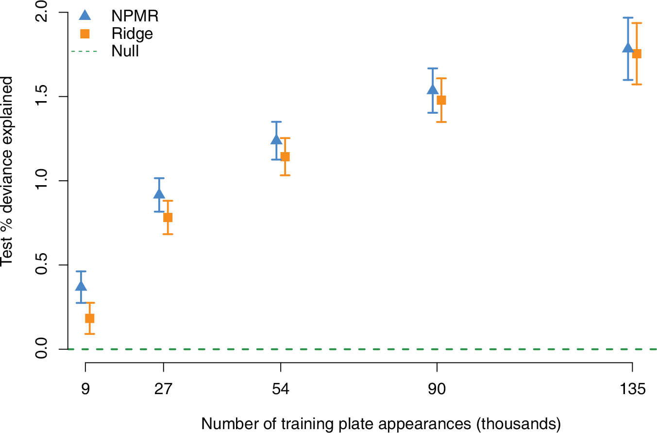
We fit NPMR and ridge regression to the baseball data, using a training sample that varied from 5% (roughly 9 000 PAs) to 75% (roughly 135 000 PAs) of the data. We used the remaining data to test the models, reporting the percentage of deviance explained in the test set, as described in Section 4. Figure 4 gives the results.

Figure 4:

Out-of-sample test performance of NPMR, ridge and null estimators on baseball plate appearance result prediction. Each estimator was trained on a fraction of the 2015 regular season data (varying from 5% to 75%) and tested on the remaining data. The error bars correspond to one standard error. The standard error of the mean test deviance is its standard deviation across test samples, divided by the square root of the number of test samples

For each training sample size, NPMR outperforms ridge regression though the difference is not statistically significant. Note that the standard errors reflect random variation in the test set, for a single training set. At the smallest sample size, NPMR, unlike ridge regression, explains significantly more test deviance than does the null estimator. There is value in improved estimation of players’ skills in small sample sizes because this can inform early-season decision-making. For all other sample sizes, both NPMR and ridge regression achieves performances which are statistically significantly better than the null. The primary benefit of NPMR relative to ridge regression is the interpretation, as described in the next section.

5.3 Interpretation

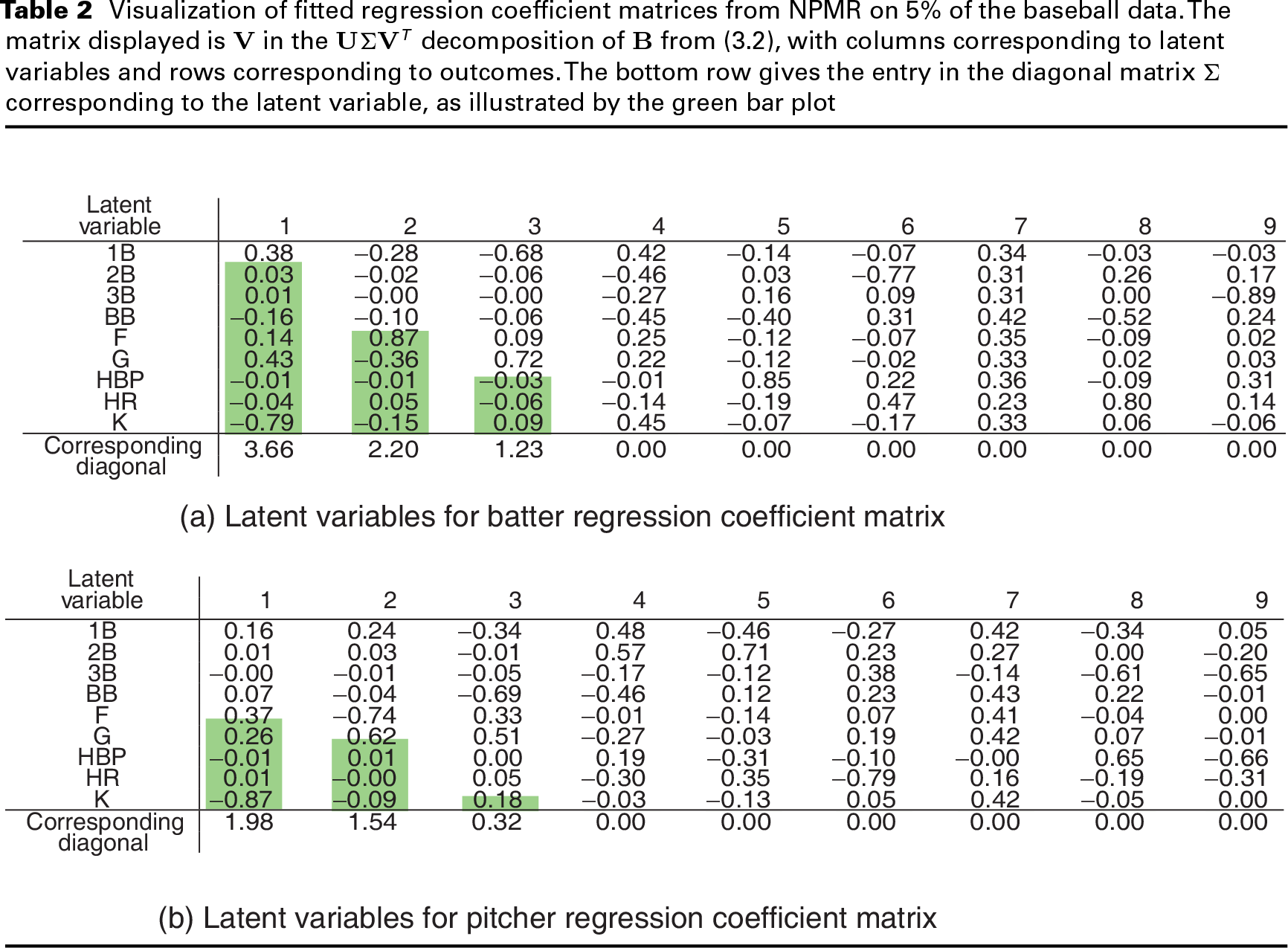
We focus on the results of fitting NPMR on 5% of the training data because there the difference between NPMR and ridge regression is the greatest (Figure 4). As the sample size increases, the need for a low-rank regression coefficient matrix is reduced, and the NPMR solution becomes more similar to the ridge solution. Table 2 visualizes the singular value decomposition of the fitted-regression coefficient submatrices corresponding to batters and pitchers. Unlike in Table 1, the diagonal entries shown in the bottom row are shrunk towards zero and cannot be interpreted in the context of percent variance explained. Note that for both batters and pitchers, six of the nine diagonal entries are exactly zero, illustrating the ability of NPMR to perform selection on the latent skills.

We observe that for both batters and pitchers, NPMR identifies three latent variables which differentiate players from one another. By construction, these latent variables are measuring separate aspects of players’ skills; across players, expression in each latent skill is uncorrelated with expression in each other latent skill. In that sense, we have identified three separate skills which characterize hitters and three separate skills which characterize pitchers. In baseball scouting parlance, these skills are called ‘tools’, but unlike the five traditional baseball tools (hitting for power, hitting for contact, running, fielding and throwing), the tools we identify are uncorrelated with one another.

Table 2:

Visualization of fitted regression coefficient matrices from NPMR on 5% of the baseball data. The matrix displayed is $V$ in the $U Σ V^{T}$ decomposition of B from (3.2), with columns corresponding to latent variables and rows corresponding to outcomes. The bottom row gives the entry in the diagonal matrix $Σ$ corresponding to the latent variable, as illustrated by the green bar plot

The interpretation of Table 2 is very attractive in the context of domain knowledge. In reading the columns of V, note that they are unique only up to a change in sign, so we can interpret positive expression in each skill as positive or negative values of the corresponding latent variable. We suggest the following interpretation of the first three latent skills for batters:

Skill 1: Patience. The loadings of the first latent variable discriminate perfectly between the TTO outcomes and the BIP outcomes described in Section 1. We label this skill as ‘patience’ because when a batter swings at fewer pitches, he is less likely to hit the ball in play.

Skill 2: Trajectory. The second latent variable distinguishes primarily between F and G, corresponding to the vertical angle of the ball off the bat.

Skill 3: Speed. The third latent variable distinguishes primarily between 1B and G. Examining the players with strong positive expression of this skill, we find fast players who are more difficult to throw out at first base on a ground ball.

From this interpretation, we learn that the primary skill which distinguishes betwen batters is how often they hit the ball into the field of play. One outcome over which batters have relatively large control is how often they swing at pitches. Among balls that are put into play, batters have less but still subtantial control over whether those are ground balls or fly balls. It is the vertical angle of the batter's swing plane, along with whether he tends to contact the top half or the bottom half of the ball, that determines his trajectory tendency. Finally, given the trajectory of the ball off the bat, the batter has relatively little control over the outcome of the PA. But to the extent that he can influence this outcome, fast runners tend to hit more singles and fewer groundouts.

Based on Table 2, we interpret the pitchers’ skills as follows:

Skill 1: Power. The first latent variable distinguishes primarily between K and F (and G), thus identifying how the pitcher gets outs. Pitchers who tend to get their outs via the strikeout are known in baseball as ‘power pitchers’.

Skill 2: Trajectory. As with batters, the second latent variable distinguishes primarily between F and G, corresponding to the batted ball's angle.

Skill 3: Command. The third latent variable distinguishes primarily between positive outcomes for the pitcher (F, G and K) and negative outcomes for the pitcher (BB and 1B), reflecting how well he is able to control his pitches.

The interpretation of the first two skills for pitchers is very similar to the interpretation of the first two skills for batters. Primarily, pitchers can influence how often balls are hit into play against them, but they exhibit less control over this than batters do. Secondarily, as with hitters, pitchers exhibit some control over the vertical launch angle of the ball off the bat. This is based on the location and movement of their pitches. The third skill, distinguishing between positive and negative outcomes, has a relatively small magnitude.

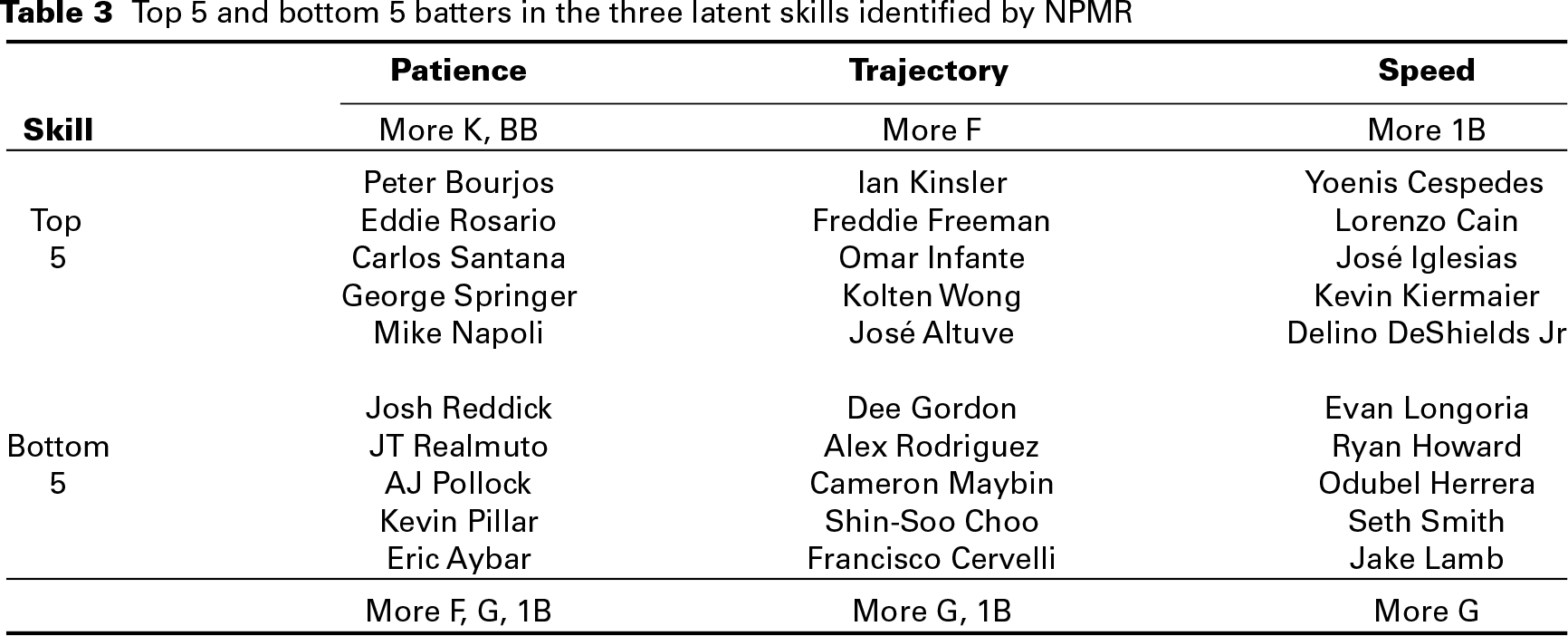
Table 3 lists the top five and bottom five players in each of the three latent batting skills learned by NPMR. These results largely match intuition for the players listed, and to the extent that they do not, it is worth a reminder that they are based on 5% of the full season's data. That is roughly equivalent to nine days’ worth of data from the six-month season. The median number of PAs per batter in the training set is 21.

Table 3:

Top 5 and bottom 5 batters in the three latent skills identified by NPMR

	Patience	Trajectory	Speed
Skill	More K, BB	More F	More 1B
	Peter Bourjos	Ian Kinsler	Yoenis Cespedes
Top	Eddie Rosario	Freddie Freeman	Lorenzo Cain
5	Carlos Santana	Omar Infante	José Iglesias
	George Springer	Kolten Wong	Kevin Kiermaier
	Mike Napoli	José Altuve	Delino DeShields Jr

	Josh Reddick	Dee Gordon	Evan Longoria
Bottom	JT Realmuto	Alex Rodriguez	Ryan Howard
5	AJ Pollock	Cameron Maybin	Odubel Herrera
	Kevin Pillar	Shin-Soo Choo	Seth Smith
	Eric Aybar	Francisco Cervelli	Jake Lamb
	More F, G, 1B	More G, 1B	More G

Table 4:

Top 5 and bottom 5 pitchers in the three latent skills identified by NPMR

	Power	Trajectory	Command
Tool	More K	More F	More F, G, K
	José Quintana	Jesse Chavez	Max Scherzer
Top	Corey Kluber	Justin Verlander	Masahiro Tanaka
5	Madison Bumgarner	Jake Peavy	Jacob deGrom
	Max Scherzer	Johnny Cueto	Rubby de la Rosa
	Clayton Kershaw	Chris Young	Matt Harvey

	John Danks	Dallas Keuchel	Mike Pelfrey
Bottom	Dan Haren	Garrett Richards	Chris Tillman
5	Cole Hamels	Sam Dyson	Eddie Butler
	Alfredo Simón	Brett Anderson	Gio Gonzalez
	RA Dickey	Michael Pineda	Jeff Samardzija
	More F, G	More G	More BB, 1B

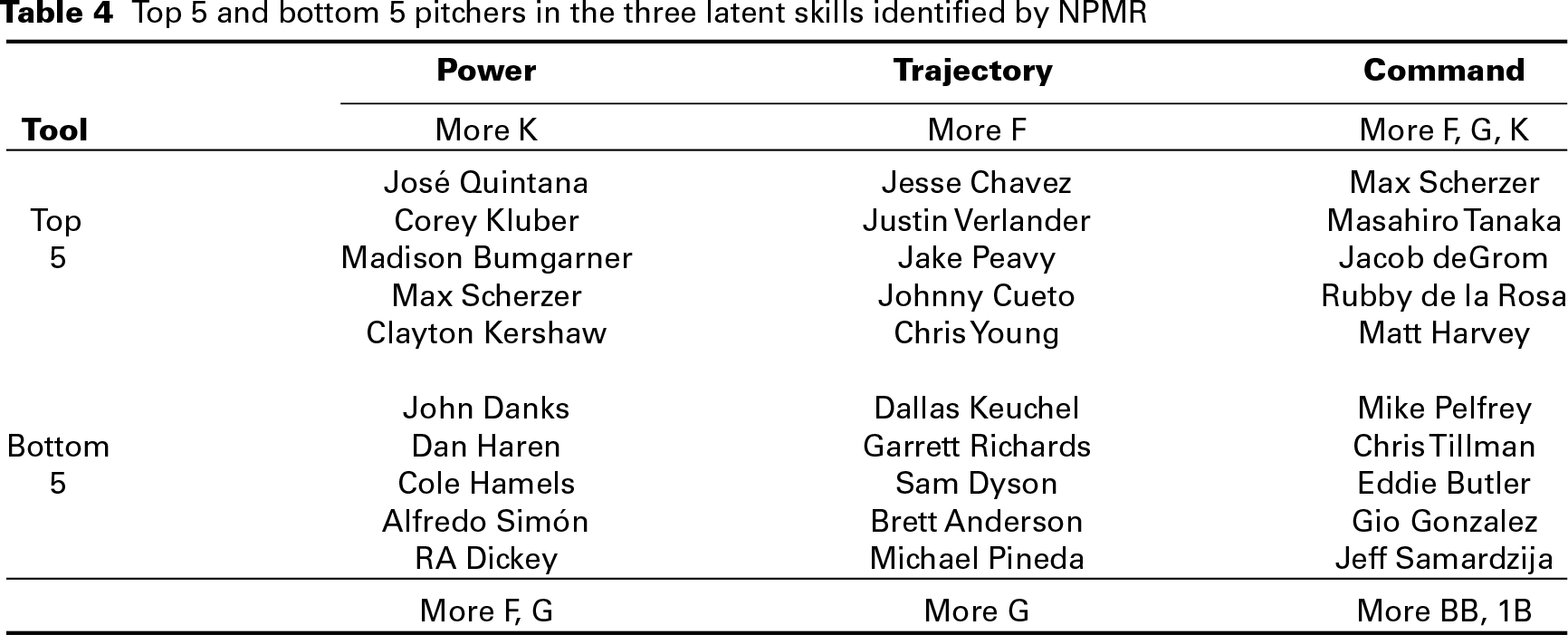
The results in Table 4, listing the top and bottom players in each of the three latent pitching skills, are more interesting. The top five power pitchers are all among the top starting pitchers in the game. All the way on the other side of the spectrum is knuckleball pitcher RA Dickey. The knuckleball is a unique pitch in baseball thrown relatively softly with as little spin as possible to create unpredictable movement. Its goal is not to overpower the opposing batter but to induce weak contact. Another interesting pitcher low on power is Cole Hamels. Two of the leading sabermetric websites, Baseball Prospectus and FanGraphs, disagree greatly on Hamels’ value. The discrepancy stems from Baseball Prospectus giving full weight to BIP outcomes, while FanGraphs ignores them. Because Hamels tends to get outs via fly balls and ground balls rather than strikeouts, FanGraphs estimates a much lower value for Hamels than Baseball Prospectus does.

5.4 Another application: Vowel data

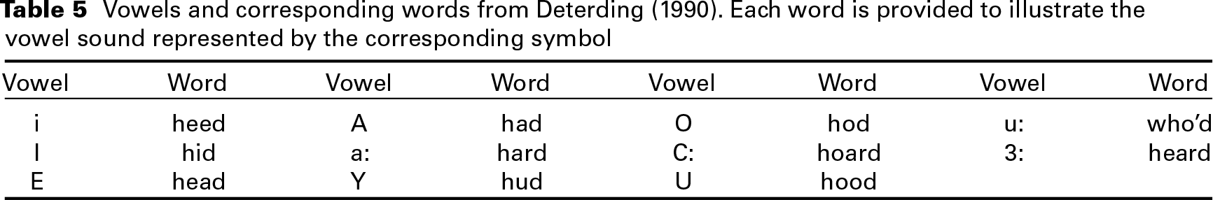
In a dataset collected by Deterding (1990) and popularized in part by Robinson (1989), the author recorded samples of 11 vowels spoken by 15 unique speakers. Each audio clip is split into 6 frames during a duration of steady audio, yielding 6 pseudo-replicates. Hence, the dataset consists of $n = 11 \times 15 \times 6 = 990$ observations. Each of these observations is represented by $p = 10$ features extracted from an audio file and is labelled as one of the vowels outlined in Table 5. Robinson (1989) split the dataset into a training sample of 528 observations and a test sample of 462 observations, stratified by speaker so that the 8 speakers in the training set are distinct from the 7 speakers in the test set.

Table 5:

Vowels and corresponding words from Deterding (1990). Each word is provided to illustrate the vowel sound represented by the corresponding symbol

Vowel	Word	Vowel	Word	Vowel	Word	Vowel	Word
i	heed	A	had	O	hod	u:	who'd
I	hid	a:	hard	C:	hoard	3:	heard
E	head	Y	hud	U	hood

We fit NPMR and ridge regression to the training data over a wide range of regularization parameters, with the results reported in Figure 5. As the regularization parameter decreases for each method, the training performance improves. The test performance initially improves and then worsens as the model overfits to the training data. We observe that over the whole solution path, for the same training deviance, NPMR consistently explains more of the test deviance than ridge regression.

Figure 5:

Results of fitting NPMR and ridge regression on vowel data. Test deviance explained is plotted against training deviance explained. Training performance serves as a surrogate for degrees of freedom in the model fit. The null prediction assigns equal probability to all categories. Error bars represent one standard error in estimation of the test deviance explained

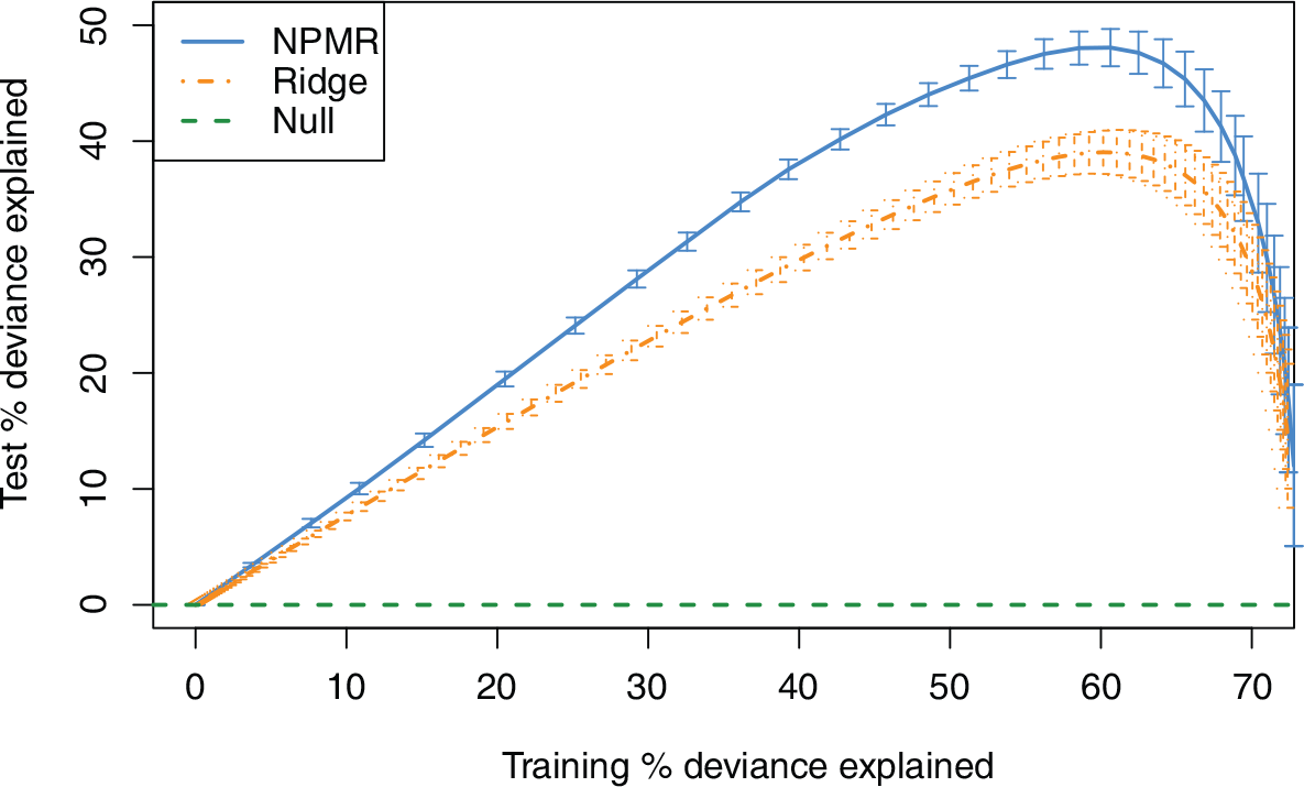
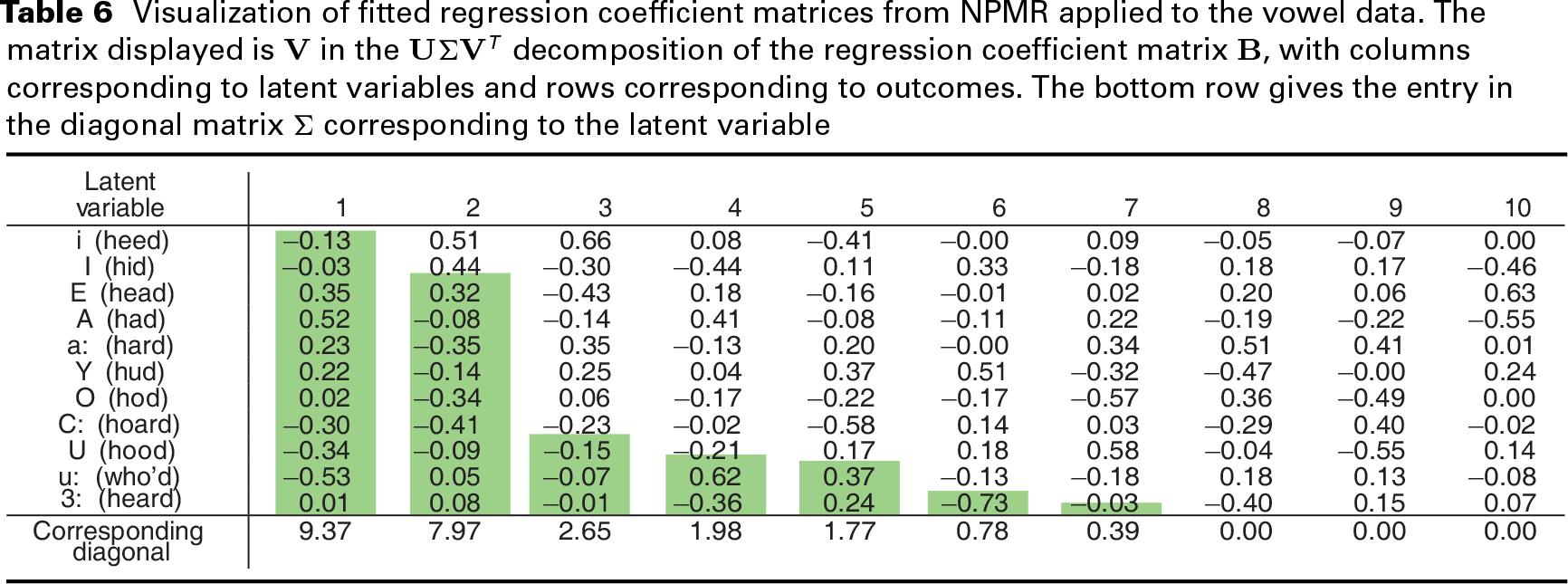
Table 6 reveals a possible explanation why NPMR outperforms ridge regression on the vowel data. For example, the results show that when the vowel i is a likely label, the vowel I is also a likely label. The first two latent variables explain a significant portion of the variance in the regression coefficients for the vowels. The first latent variable distinguishes between two groups of vowels, with C:, U and u: having the most negative values and E, A, a: and Y having the most positive values. NPMR beats ridge regression here by leveraging a hidden structure among response classes.

Table 6:

Visualization of fitted regression coefficient matrices from NPMR applied to the vowel data. The matrix displayed is V in the UΣV^T decomposition of the regression coefficient matrix B, with columns corresponding to latent variables and rows corresponding to outcomes. The bottom row gives the entry in the diagonal matrix Σ corresponding to the latent variable

6 Discussion

The potential for reduced-rank multinomial regression to leverage the underlying structure among response categories has been recognized in the past. But the computational cost for the state-of-the-art algorithm for fitting such a model is so great as to make it infeasible to apply to a dataset as large as the baseball play-by-play data in the present work. Using a convex relaxation of the problem, by penalizing the nuclear norm of the coefficient matrix instead of its rank, leads to better results.

The interpretation of the results on the baseball data is promising in how it coalesces with modern baseball understanding. Specifically, the NPMR model has quantitative implications on leveraging the structure in PA outcomes to better jointly estimate outcome probabilities. Additional application to vowel recognition in speech shows improved out-of-sample predictive performance, relative to ridge regression. This matches the intuition that NPMR is well suited to multinomial regression in the presence of a generic structure among the response categories. We recommend the use of NPMR for any multinomial regression problem for which there is some non-ordinal structure among the outcome categories.

Acknowledgements

The authors would like to thank Hristo Paskov, Reza Takapoui and Lucas Janson for helpful discussions, as well as Balasubramanian Narasimhan for computational assistance.We are grateful to Andreas Groll and an anonymous reviewer for a careful review and comments that led to improvements to this work.

Declaration of conflicting interests

The author(s) declared no potential conflicts of interest with respect to the research, authorship, and/or publication of this article.

Funding

The author(s) received no financial support for the research, authorship, and/or publication of this article.

Appendix

Identifiability of multinomial logistic regression model

We observe in Section 2 that the model (2.1) is not identifiable: For any $a \in$ and $c \in ℝ^{p}$ ,

\frac{e^{α_{k} - a + x_{i}^{T} (β_{k} - c)}}{\sum_{ℓ = 1}^{K} e^{α_{ℓ} - a + x_{i}^{T} (β_{ℓ} - c)}} = \frac{e^{- α - x_{i}^{T} c} e^{α_{k} + x_{i}^{T} β_{k}}}{e^{- α - x_{i}^{T} c} \sum_{ℓ = 1}^{K} e^{α_{ℓ} + x_{i}^{T} β_{ℓ}}} = \frac{e^{α_{k} + x_{i}^{T} β_{k}}}{\sum_{ℓ = 1}^{K} e^{α_{ℓ} + x_{i}^{T} β_{ℓ}}}

Hence,

(α, B)

and

(α - a 1_{K}, B - c 1_{K}^{T})

have the same likelihood. The ridge penalty in (3.7) provides a natural resolution. Any solution to this problem must satisfy

{‖ B ‖}_{F}^{2} = \min_{c \in ℝ^{p}} {‖ B - c 1_{K}^{T} ‖}_{F}^{2},

(A.1)

because otherwise B can be replaced by

B - c 1_{K}^{T}

with a smaller norm but the same likelihood, and hence a lesser objective. Note that the optimization problem on the right-hand side of (A.1) is separable in the entries of

c

and has the unique solution

c^{*} = \frac{1}{K} B 1_{K}

, meaning that the rows of B in the solution must have mean zero. The unpenalized intercept

α

still lacks identifiability, but we may take it to have mean zero as well.

Similarly, the NPMR solution must satisfy

{‖ B ‖}_{*} = \min_{c \in ℝ^{p}} {‖ B - c 1_{K}^{T} ‖}_{*} .

(A.2)

Whether this optimization problem always (for any

B \in ℝ^{p \times K}

) has a unique solution is an open question. We speculate that it does and that the unique solution is

c^{*} = \frac{1}{K} B 1_{K}

. As evidence, each fit of NPMR in the present manuscript has a solution with zero-mean rows. As further evidence, we have used the MATLAB software CVX (Grant et al., 2008) to solve (A.2) for several randomly generated matrices B, and each time the solution has been

c^{*} = \frac{1}{K} B 1_{K}

Note that $c^{*} = \frac{1}{K} B 1_{K}$ must always be a solution to (A.2). To see this, note that

B - c^{*} 1_{K}^{T} = B - \frac{1}{K} B 1_{K} 1_{K}^{T} = B (I - \frac{1}{K} 1_{K} 1_{K}^{T}) = B (I - H),

where

H = 1_{K} {(1_{K}^{T} 1_{K})}^{- 1} 1_{K}^{T}

is a projection matrix. Hence,

I - H

is also a projection matrix and has spectral norm (maximum singular value)

| | I - H | |_{\infty} = 1

. By Hölder's inequality for Schatten

p

-norms (Bhatia, 1997),

| | B (I - H) | |_{*} \leq | | B | |_{*} | | I - H | |_{\infty} = | | B | |_{*},

so for any

B \in ℝ^{p \times K}

| | B - \frac{1}{K} B 1_{K} 1_{K}^{T} | |_{*} \leq | | B | |_{*} .

In other words, the nuclear norm can always be decreased, or at least not increased, by centreing the rows to have mean zero.

The problem with a lack of identifiability in the multimonial regression model comes in the interpretation of the regression coefficients. When comparing coefficients across variables for the same outcome class, it is concerning that an arbitrary increase in either coefficient can correspond to the same fitted probabilities (if that same increase applies to all other coefficients for the same variable). This does not apply to any of the interpretation in Section 5.3, but in the absence of certainty that there is a unique solution to (A.2), we take the NPMR solution to be the one for which the mean of $α$ and the row means of B are zero.

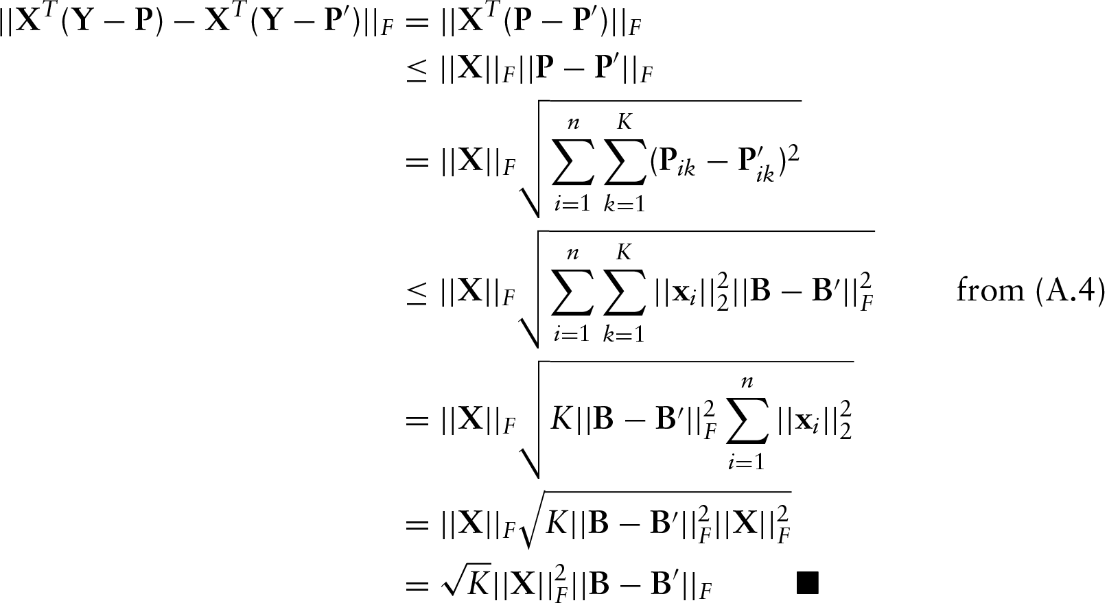
Proof of Lipschitz condition for multinomial log likelihood

We prove that the multinomial log-likelihood $ℓ (α, B; X, Y)$ from (3.2) has Lipschitz gradient with constant $L = \sqrt{K} | | X | |_{F}^{2}$ . Assume (without loss of generality) that the covariate matrix $X$ has a column of 1s encoding the intercept, so $α = 0$ . The gradient of $ℓ (B; X, Y)$ with respect to B is given by $X^{T} (Y - P)$ , where $Y$ and $P$ are defined as in (3.4). What we must show is that, for any $B, B^{'} \in ℝ^{p \times K}$ :

| | X^{T} (Y - P) - X^{T} (Y - P^{'}) | |_{F} \leq \sqrt{K} | | X | |_{F}^{2} | | B - B^{'} | |_{F} .

(A.3)

Recall that P is a function of B, so

P^{'}

corresponds to

B^{'}

Consider a single entry $P_{ik}$ of P. Note that the gradient of $P_{ik}$ with respect to B is given by $x_{i} w_{ik}^{T}$ , where $w_{ik} \in R^{p}$ and

(w_{ik})_{j} = {\begin{matrix} - P_{ik} P_{ij} & j \neq k \\ P_{ik} (1 - P_{ik}) & j = k \end{matrix} . .

For any

P \in (0, 1)^{n \times K}

| | w_{ik} | |_{2} \leq | | w_{ik} | |_{1} = P_{ik} (1 - P_{ik}) + P_{ik} \sum_{j \neq k} P_{jk} = 2 P_{ik} (1 - P_{ik}) \leq \frac{1}{2} .

This implies that the norm of the gradient of

P_{ik}

is bounded above by the inequality

| | x_{i} w_{ik}^{T} | |_{F} \leq | | x_{i} | |_{2} | | w_{ik}^{T} | |_{F} \leq | | x_{i} | |_{2}

. So for any

B, B^{'} \in ℝ^{p \times K}

| P_{ik} - P_{ik}^{'} | \leq | | x_{i} | |_{2} | | B - B^{'} | |_{F} .

(A.4)

Now we are ready to prove (A.3).

\begin{matrix} {‖ X^{T} (Y - P) - X^{T} (Y - P^{'}) ‖}_{F} & = ‖ X^{T} (P - P^{'}) ‖ \\ \leq {‖ X ‖}_{F} {‖ P - P^{'} ‖}_{F} \\ = {‖ X ‖}_{F} \sqrt{\sum_{i = 1}^{n} \sum_{k = 1}^{K} {(P_{i k} - {P^{'}}_{i k})}^{2}} \\ \leq {‖ X ‖}_{F} \sqrt{\sum_{i = 1}^{n} \sum_{k = 1}^{K} {‖ x_{i} ‖}_{2}^{2} {‖ B - B^{'} ‖}_{F}^{2}} from (A .4) \\ = {‖ X ‖}_{F} \sqrt{K {‖ B - B^{'} ‖}_{F}^{2} \sum_{i = 1}^{n} {‖ x_{i} ‖}_{2}^{2}} \\ = {‖ X ‖}_{F} \sqrt{K {‖ B - B^{'} ‖}_{F}^{2} {‖ X ‖}_{F}^{2}} \\ \sqrt{K} {‖ X ‖}_{F}^{2} {‖ B - B^{'} ‖}_{F} \end{matrix}

References

Albert

(2016) Improved component predictions of batting and pitching measures. Journal of Quantitative Analysis in Sports , 12, 73–85.

Anderson

(1984) Regression and ordered categorical variables. Journal of the Royal Statistical Society B , 46, 1–30.

Baumer

Zimbalist

(2014) The Sabermetric Revolution . Philadelphia, PA: University of Pennsylvania Press.

Bhatia

(1997) Matix Analysis . New York, NY: Springer.

Brown

(2008) In-season prediction of batting averages: A field test of empirical Bayes and Bayes methodologies. The Annals of Applied Statistics , 2, 113–152.

Chen

Dong

Chan

K-S

(2013) Reduced rank regression via adaptive nuclear norm penalization. Biometrika , 100, 901–920.

Deterding

(1990) Speaker normalisation for automatic speech recognition. PhD dissertation, University of Cambridge, UK.

Efron

Morris

(1975) Data analysis using Stein's estimator and its generalizations. Journal of the American Statistical Association , 70, 311–319.

Friedman

Hastie

Tibshirani

(2010) Regularization paths for generalized linear models via coordinate descent. Journal of Statistical Software , 33, 1–22.

10.

Grant

Boyd

(2008) CVX: Matlab software for disciplined convex programming. CVX Research. URL http://www.cvxr.com/(last accessed on 1 May 2018).

11.

Greenland

(1994) Alternative models for ordinal logistic regression. Statistics in Medicine , 13, 1665–1677.

12.

Hastie

Tibshirani

Friedman

(editors) (2009) The elements of statistical learning: Data mining, inference and prediction. In Springer Series in Statistics, 2nd edition. New York: Springer.

13.

Hastie

Tibshirani

Wainwright

(editors) (2015) Statistical learning with sparsity: The lasso and its generalizations. In Monographs on Statistics and Applied Probability, 1st edition. New York: CRC Press.

14.

Judge

BP Stats Team (2015) DRA: An in-depth discussion. URL http://www.baseballprospectus.com/article.php?articleid=26196(last accessed on 1 May 2018).

15.

Likert

(1932). A technique for the measurement of attitudes. Archives of Psychology , 140, 1–55.

16.

Morris

(1983) Parametric empirical Bayes inference: Theory and applications. Journal of the American Statistical Association , 78, 47–55.

17.

Nesterov

(2007) Gradient methods for minimizing composite objective function (Technical report 2007076). Universite catholique de Louvain, Center for Operations Research and Econometrics (CORE).

18.

Null

(2009) Modeling baseball player ability with a nested Dirichlet distribution. Journal of Quantitative Analysis in Sports , 5.

19.

R Core Team (2016) R: A language and environ- ment for statistical computing . Vienna: R Foundation for Statistical Computing. URL http://www.R-project.org/.

20.

Robinson

(1989) Dynamic error propagation networks. PhD dissertation, University of Cambridge, UK.

21.

Tibshirani

(1996) Regression shrinkage and selection via the lasso. Journal of the Royal Statistical Society B , 58, 267–288.

22.

Tutz

Gertheiss

(2016) Regularized regression for categorical data (with discussion and rejoinder). Statistical Modelling , 16, 161–260.

23.

Yee

(2010) The VGAM package for categorical data analysis. Journal of Statistical Software , 32, 1–34.

24.

Yee

Hastie

(2003) Reduced-rank vector generalized linear models. Statistical Modelling , 3, 15–41.