Multivariate calibration with robust signal regression

Abstract

Motivated by a multivariate calibration problem from a soil characterization study, we proposed tractable and robust variants of penalized signal regression (PSR) using a class of non-convex Huber-like criteria as the loss function. Standard methods may fail to produce a reliable estimator, especially when there are heavy-tailed errors. We present a computationally efficient algorithm to solve this non-convex problem. Simulation and empirical examples are extremely promising and show that the proposed algorithm substantially improves the PSR performance under heavy-tailed errors.

Keywords

Huber loss multivariate calibration P-splines robust regression signal regression

1 Introduction

We revisit the information-rich regression problem where regressors are ordered and ensemble a signal or curve, for instance, when a scalar response is regressed onto a spectra, curve, log-periodogram or time series. Such problems usually lead to the paradox of knowing too much information, since resulting standard regression approaches are commonly ill-conditioned. Specifically we consider settings where the number of regressors or discrete digitizations of the signal ( $p$ ) (generally) exceed the number of observations ( $m$ ) or $p ≫ m$ . In the chemometric community, this is referred to as the multivariate calibration problem, but we will freely interchange this term with signal regression. Notationally, we have

μ = E (y) = X β,

(1.1)

where $y$ denotes the $m$ -dimensional response vector, $X$ the $m \times p$ regressor matrix (each row consisting of a digitized signal) and $β$ the $p$ -dimensional unknown coefficient vector. Implicitly, there is an ordering index associated with the regressors, and without loss of generality can be denoted as the vector $1 : p$ . Although the least-squares objective function has a familiar form, that is, $S (β) = | | y - X β | |^{2}$ , there is not a unique solution. Naturally, some constraints are needed to solve such problem, and there exist a vast number of proposals, including principal components, partial least squares, support vector machines, genetic algorithms and orthogonal signal correction, among many others. Our intention is not to resolve further all of the cross-comparisons, but rather to focus on a tractable and sensible robust variant of penalized signal regression (PSR), an approach first proposed by (Marx and Eilers, 1999). In addition, our work generalizes the robust penalized regression splines by Lee and Oh (2007). A recap of PSR can be found in Section 3, but the essence of PSR is to project the ordered high-dimensional signal coefficient vector onto rich B-spline basis using equally spaced knots. A P-spline approach (Eilers and Marx, 1996) is taken in that the basis coefficients are constrained using a difference penalty, and the amount of smoothness is enforced by a tuning parameter chosen based on externally cross-validated prediction error. The main objective of this article is to present tractable and robust variants of PSR using a class of non-convex Huber-like criteria as the loss functions. An efficient computational algorithm is proposed to solve this non-convex problem. Simulation and empirical examples show the proposed algorithm performs well under heavy-tailed errors and is suitable for large-scale problems.

1.1 A brief literature overview

Although much research has been done on robust estimation in the context of smoothing, as far as we know, little or no work has been done in implementing robust smoothing into the multivariate calibration problem, for example, using robust variants of PSR. An assortment of loss functions—in addition to squared error loss—have been applied to the penalized spline and regression splines. For instance, Huber (1979) and Cox (1983) proposed to use M-type robust smoothing with cubic regression splines. Other articles on robust smoothing and nonparametric regression include Hardle and Gasser (1984), Silverman (1985) and Hall and Jones (1990). Eilers and de Menezes (2005) applied quantile smoothing with $L_{1}$ loss on comparative genomic hybridization (CGH) data. Robust penalized regression spline was explored by Lee and Oh (2007), in which Huber loss was used for bivariate smoothing. In Section 6.3, we fully draw the connection between our work and that of Lee and Oh (2007). They also applied the robust penalized regression spline to an additive mixed modelling setting. Tharmaratnam et al. (2010) studied S-estimation for penalized regression splines. A recent paper by Kneib (2013) discussed the semiparametric regression models that go beyond the mean and squared error loss, such as quantile and expectile regressions.

2 The motivating example

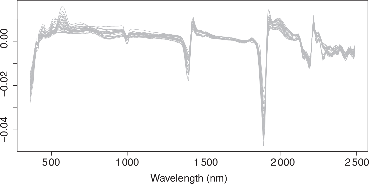
The dataset contains a total of 675 soil samples collected from Seward County (Nebraska), Kern County (California) and Lubbock County (Texas) in 2014. In particular, 75 sampling points were randomly selected within a single agricultural field in each of these states, and soil samples were collected at three depths (0–15 cm, 15–30 cm and 30–45 cm). Ten physicochemical properties were measured for all 675 soil samples. They are soil cation exchange capacity (CEC), electrical conductivity (EC), total nitrogen level, total carbon level, loss on ignition (LOI), soil organic matter (SOM), clay, sand, silt and soil pH level. Since LOI and SOM are highly correlated, LOI was removed from the study. All the soil samples were scanned using a portable VisNIR spectroradiometer with a spectral range of 350–2 500 nm. After smoothing and taking first order derivatives, the processed reflectance spectra were measured from 360 nm to 2 490 nm at 10 nm intervals. The purpose of the study is to predict the nine soil physicochemical properties from its reflectance spectra, estimating many soil properties from the same optical regressor. One feature of this dataset, which motivates our study, is that the soil sampled had widespread variation in physicochemical properties. This dataset was originally used in Wang et al. (2015). Figure 1 shows a random sample of 30 spectra from the dataset.

Figure 1:

Thirty sample (first derivative) spectra for the soil data

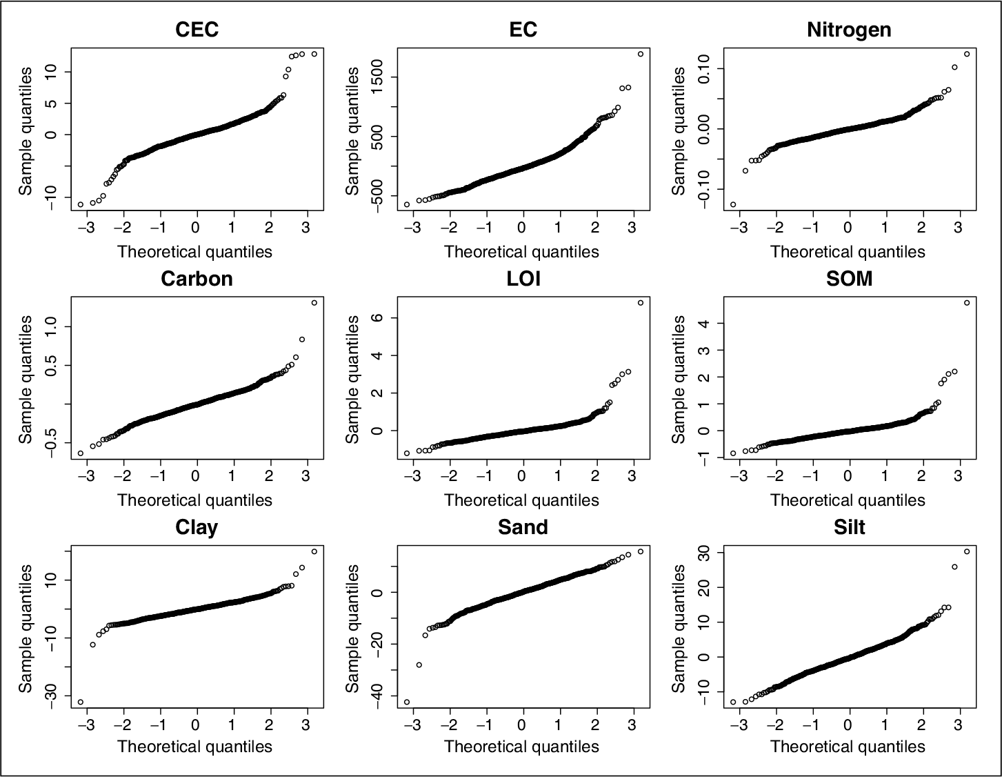
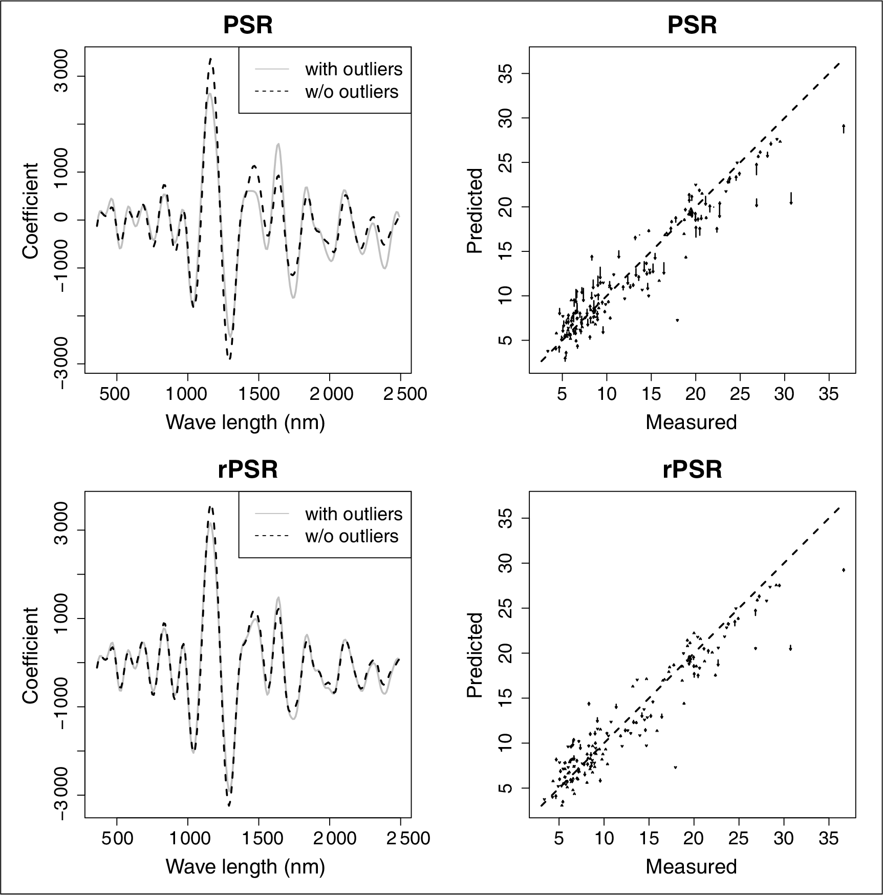
For initial illustration, PSR was applied to the spectral data to predict each of the nine responses. Details of this technique are recapped in the next section. Figure 2 shows the corresponding normal quantile–quantile plots of the PSR residuals, by response variables. We find that all of the models contain some outlying residuals. As with other least-squares methods, PSR suffers from the heavy-tailed errors or outliers in the response. In this article, we proposed to use robust loss function within the PSR, and we will refer to this method as robust PSR or rPSR. Figure 3 compares the coefficient plots and prediction on test samples with and without the outliers in the CEC case for PSR and rPSR. Note that the outliers in the training samples are those whose standardized residuals are greater than 3 in absolute value. In CEC case, there are less than 2% of these outlying samples in the training set (which itself consists of 75% of the entire dataset). We find that the PSR coefficients and its prediction on test samples are more sensitive to the existing outliers than the ones of our proposed rPSR. A brief review of PSR follows in the next section, and Section 4 outlines our robust variant or rPSR.

Figure 2:

The normal quantile-quantile plots of the residuals for nine response variables after fitting penalized signal regression using P-splines

Figure 3:

The coefficient plots with (solid grey) and without (black dash) the outliers for PSR (top left) and rPSR (bottom left) when modelling the response CEC; the prediction plots on test samples with and without the outliers for PSR (top right) and rPSR (bottom right). The arrows start from the predicted CEC values including all the training samples (with outlying samples) to the predicted CEC values excluding the samples with outlying residuals

3 Recap: Penalized signal regression

As mentioned in Section 1, the essence of PSR is to use a signal regressor matrix $X$ (each row is an ordered signal) to predict a scalar response $y$ . Figure 1 provides a visual representation of $X$ of dimension $675 \times 214$ , with the indexing variable of length $p = 214$ (360–2 490 nm, in units of 10 nm). Notable for the full dataset of $m = 675$ : the problem is not ill-posed in a strict sense since then $m > p$ , but clearly the signal channels offer high collinearity. Moreover, if the signal had been measured on a finer grid (e.g., with a more precise instrument), we would not expect the figure to change very much—which is a tribute to the inherent redundancy across neighbouring columns of $X$ . The beauty of PSR is that it can routinely accommodate such severe collinearity, and can naturally handle fully ill-posed problems ( $p ≫ m$ ). Given the ordering index, the goal of PSR is to force $β$ to be smooth, by first projecting it onto a rich B-spline basis and then putting a difference penalty on the adjacent B-spline coefficients, thereby making the problem well-posed through the spirit of P-splines (Eilers and Marx, 1996). Hence, we have $β = B α$ . The dimension of $B$ is $p \times n$ and is built along the indexing variable, with $n$ coefficients in $α$ . Our view is that smoothness can be viewed as one of many constraints towards regularization; it is either a sensible choice or one that is non-detrimental towards prediction.

More specifically, the P-spline step in PSR places the penalty directly on $α$ and minimizes the following modified objective:

S (α) = | | y - XB α | |^{2} + λ | | D α | |^{2},

(3.1)

and we find the difference matrix $D$ penalizes differences on $α$ . Minimizing $S (α)$ yields

(B^{'} X^{'} XB + λ D^{'} D) α = B^{'} X^{'} y .

Denoting the $U = XB$ as the effective regressors of dimension $m \times n$ , we have the following explicit solution

\begin{matrix} \hat{α} & = & (U^{'} U + λ D^{'} D)^{- 1} U^{'} y \\ \hat{β} & = & B \hat{α}, \end{matrix}

(3.2)

which are functions of the tuning parameter $λ$ . Efficiently, $U^{'} U$ and $U^{'} y$ only need to be computed once, even while tuning smoothness through $λ$ . The optimal choice of $λ$ can be made using cross-validation. Thus far, we have not included an intercept term in the model, which can be easily included, that is, $μ = β_{0} + X β = β_{0} + U α$ . Note that some care has to be taken to ensure $β_{0}$ is not penalized. As $X$ is now augmented with a column of ones, $λ D^{'} D$ in (3.2) needs to be replaced with $block diagonal (0, λ D^{'} D)$ .

4 Methodology

4.1 Generalized Huber loss

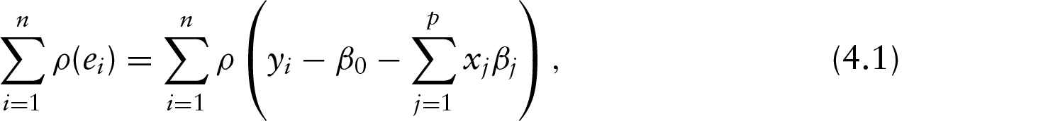
The least-squares estimate works well in the presence of normal error or even in situations where the error distribution is reasonably continuous, symmetric and not too heavy tailed. However, with departures from the above, the least-squares criterion can lead to poor results, especially for heavy-tailed errors and outliers in the response. A ‘robust’ statistical procedure is often able to provide useful information even when some of the assumptions are not applicable. In regression analysis, a convenient approach is simply to remove the influential observations from the least-squares fit, whereas alternatively ‘robust regression’ employs a criterion that is more resistant (to unusual observations) than those found using least squares. A tried-and-true method of robust regression is ‘ $M$ -estimation’, introduced by Huber (1964). The general $M$ -estimator minimizes the objective function

i = 1 n ρ (e_{i}) = i = 1 n ρ (y_{i} - β_{0} - j = 1, p, x_{j}, β_{j}),

(4.1)

where the function $ρ$ has the following properties: (a) $ρ (e) \geq 0$ , (b) $ρ (0) = 0$ , (c) $ρ (e) = ρ (- e)$ and (d) $ρ (e_{i}) \geq ρ (e_{j})$ for $| e_{i} | > | e_{j} |$ . For example, for least-squares estimation uses $ρ (e) = e^{2}$ . (Huber 1981) further described a well-known robust $M$ -estimator employing a loss function that is less affected by very large residual values. The Huber criterion can be written as

\begin{matrix} ρ_{H} (e) = \{\begin{matrix} e^{2} & | e | < K \\ 2 K | e | - e^{2} = K^{2} + 2 K (| e | - K) & | e | \geq K . \end{matrix} \end{matrix}

(4.2)

The parameter $K$ defines the point of transition from quadratic to linear loss. Specifically, errors smaller than $K$ get squared, while larger errors only increase the loss linearly.

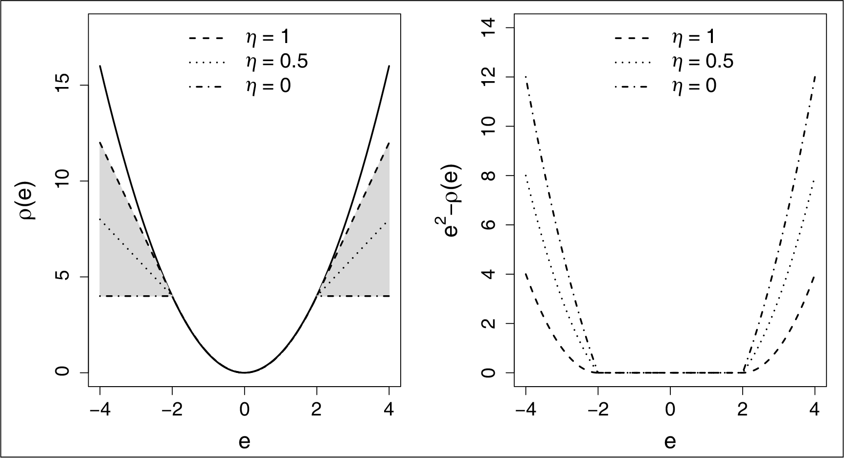
Li and Yu (2009) generalized the Huber loss criterion described in (4.2) to a class of $M$ -estimators, called ‘generalized Huber criterion’ as follows

\begin{matrix} ρ_{η} (e) = \{\begin{matrix} e^{2} & | e | < K \\ K^{2} + 2 η K (| e | - K) & | e | \geq K, \end{matrix} \end{matrix}

(4.3)

where $0 \leq η \leq 1$ . The left panel of Figure 4 illustrates the family of generalized Huber loss with three different values of $η$ at $K = 2$ . The black solid curve is the square loss function. The grey-shaded region represents the region for all the possible generalized Huber loss $ρ_{η} (e)$ with $η$ ranging from zero to one. The right panel of the same figure shows the difference between squared error loss and $ρ_{η} (e)$ .

Figure 4:

Illustration of generalized Huber loss with three different values of $η$ at $K = 2$ (left) and the corresponding trailing convex functions (right). The three generalized Huber loss functions can be expressed as the differences of the squared error loss (solid curve, left) and the corresponding trailing functions (right)

The class of generalized Huber loss falls into the category of ‘redescending $M$ -estimator’, which includes: Tukeys bi-weight, $S$ -estimators (Maronna et al., 2006) and $t$ -type scores (He et al., 2000). Clearly, the smaller the $η$ , then the more robust the loss function is against the outliers in error. When $η$ is one, the generalized Huber loss $ρ_{η = 1}$ is the Huber loss $ρ_{H}$ . The truncated least-squares criterion corresponds to $ρ_{η = 0}$ , which approximates the Tukey's bi-weight $M$ -estimator. Although the generalized Huber criterion is not convex (in $e \in ℝ$ ) for $0 \leq η < 1$ , it can be expressed as a difference of two convex functions (of $e$ ) as follows:

ρ η (e) = e^{2} - I (| e | 〉 k) [〉 e^{2} + 2 η K (K - | e |) - k^{2}],

(4.4)

where $I (\cdot)$ is an indicator function, equal to one when condition holds, zero otherwise. Note that the leading convex function is the square loss function. In Figure 4, the right panel further shows the second term on the right side of (4.4), which is convex and $K$ -insensitive (i.e., it is a constant within the range $[- K, K]$ ).

4.2 Difference convex programming

The difference convex (d.c.) programming, developed by An and Tao (1997), addresses the problem of minimizing an objective function, which can be expressed as a difference of two convex functions, on the whole space. Consider minimizing an objective function $h (a)$ which is a difference of two convex functions, that is, $h (a) = h_{1} (a) - h_{2} (a)$ where both $h_{1} (a)$ and $h_{2} (a)$ are convex in $a$ . The key idea of d.c. programming is to construct a sequence of subproblems, which are obtained by replacing the trailing convex function, for example, $h_{2} (a)$ , by its first order approximation function $h_{2} (a^{(o)}) + ⟨ a - a^{(o)}, ▽ h_{2} (a^{(o)}) ⟩$ and solve them iteratively, where $▽ h_{2} (a^{(o)})$ is the subgradient of $h_{2} (a)$ at $a^{(o)}$ with respect to $a$ . Specifically, given the current solution for the subproblem $a^{cur}$ , the new subproblem solves

a^{new} = \arg min_{a} h_{1} (a) - [h_{2} (a^{cur}) + ⟨ a - a^{cur}, ▽ h_{2} (a^{cur}) ⟩] .

(4.5)

Note that after removing the constant terms in (4.4), minimizing the subproblem is equivalent to

a^{new} = \arg min_{a} h_{1} (a) - ⟨ a, ▽ h_{2} (a^{cur}) ⟩ .

(4.6)

4.3 Algorithm of robust P-splines

In this article, we suggest to replace the least-square criterion by the generalized Huber criterion described in (4.3) within the PSR framework. Hence the robust PSR (rPSR) minimizes

Q (α) = \{i = 1 m ρ_{η} (y_{i} - U_{i}^{'} α)\} + λ α^{'} D_{d}^{'} D_{d} α,

(4.7)

which can be represented as a difference of two convex functions as follows:

Q (α) = h_{1} (α) - h_{2} (α), W H E R E

(4.8)

h_{1} (α) = \sum_{i = 1}^{m} e_{i}^{2} + λ α^{'} D^{'} D α

(4.9)

h_{2} (α) = \sum_{i = 1}^{m} I (| e_{i} | > K) [e_{i}^{2} + 2 η K (K - | e_{i} |) - K^{2}],

(4.10)

and $e_{i} = y_{i} - U_{i}^{'} α$ . The subgradient of $h_{2} (α)$ with respect to $α$ is

▽ h_{2} (α) = \frac{\partial h_{2}}{\partial e} \cdot \frac{\partial e}{\partial α} = - 2 i = 1 m I (| e_{i} | > K) [e_{i} - η K Sign (e_{i})] U_{i},

(4.11)

where $Sign (a)$ is the sign function, equal to $1$ if $a$ is positive, $- 1$ if $a$ is negative and $0$ otherwise. The vector $U_{i}^{'}$ is the $i$ th row of $U = XB$ , with $n$ elements ${u_{ij}}_{j = 1}^{n}$ . Let $V$ be a column vector of length $m$ with elements ${I (| e_{i} | > K) [e_{i} - η K Sign (e_{i})]}_{i = 1}^{m}$ . It follows that the right side of (4.7) can be expressed as $- 2 U^{'} V$ . The inner product of $α$ and subgradient $▽ h_{2} (α)$ is then

⟨ α, ▽ h_{2} (α) ⟩ = - 2 α^{'} U^{'} V .

(4.12)

Through d.c. programming, the minimization of the objective function (4.6) translates to the minimizing of a sequence of subproblems

\hat{α} = \arg min_{α} (Y - U α)^{'} (Y - U α) + λ α^{'} D^{'} D α + 2 α^{'} U^{'} V .

(4.13)

Setting the first order derivative of the right side of (4.9) to zero, we have the closed form of the solution

\hat{α} = {(U^{'} U + λ D^{'} D)}^{- 1} U^{'} (Y - V) = {(U^{'} U + λ D^{'} D)}^{- 1} U^{'} Y^{A} .

(4.14)

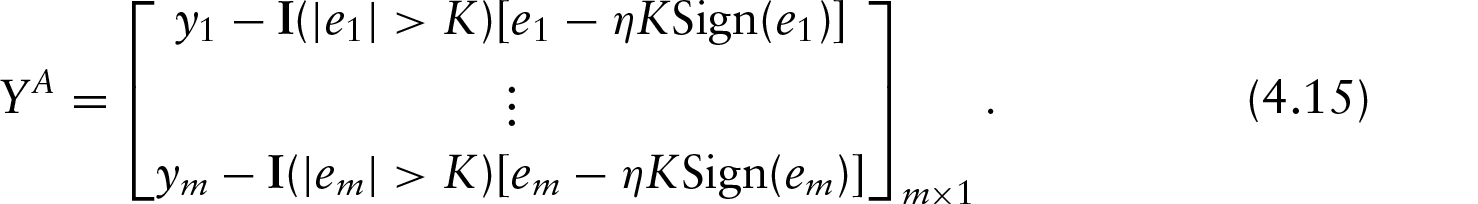
The right side of (4.10) further shows that the subproblem solution is itself a modified PSR solution, one with the adjusted responses $Y^{A}$ defined as

\begin{matrix} Y^{A} = {[\begin{matrix} y_{1} - I (| e_{1} | > K) [e_{1} - η K Sign (e_{1})] \\ ⋮ \\ y_{m} - I (| e_{m} | > K) [e_{m} - η K Sign (e_{m})] \end{matrix}]}_{m \times 1} . \end{matrix}

(4.15)

Note that only the observations with the residuals greater than $K$ (in absolute value) will be ‘adjusted’. Further, if $K$ is greater than all the residuals ${e_{i}}$

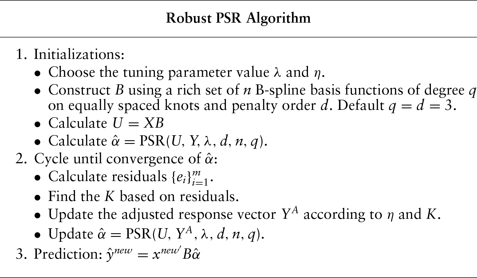
Robust PSR Algorithm

1. Initializations:

Choose the tuning parameter value $λ$ and $η$ .

Construct $B$ using a rich set of $n$ B-spline basis functions of degree $q$ on equally spaced knots and penalty order $d$ . Default $q = d = 3$ .

Calculate $U = XB$

Calculate $\hat{α} = PSR (U, Y, λ, d, n, q)$ .

2. Cycle until convergence of $\hat{α}$ :

Calculate residuals ${e_{i}}_{i = 1}^{m}$ .

Find the $K$ based on residuals.

Update the adjusted response vector $Y^{A}$ according to $η$ and $K$ .

Update $\hat{α} = PSR (U, Y^{A}, λ, d, n, q)$ .

3. Prediction: ${\hat{y}}^{new} = x^{{new}^{'}} B \hat{α}$

From the above algorithm, we have the following remarks: (a) For initial $\hat{α}$ , we use the PSR estimate (with the same value of $λ$ ). Note that we deliberately fix the tuning parameter $λ$ during the iterations to minimize the objective function (4.6); (b) Let ${\hat{α}}_{j}^{pre}$ and ${\hat{α}}_{j}^{cur}$ be the $j th$ element of the $α$ vector for the previous and current iteration. The algorithm terminates when $max {| ({\hat{α}}_{j}^{cur} - {\hat{α}}_{j}^{pre}) / {\hat{α}}_{j}^{pre} |}_{j = 1}^{n} < ε$ , where $ε$ is a pre-specified convergence tolerance. We set $ε$ at $10^{- 6}$ here; (c) The cut-off value $K$ in the generalized Huber criterion is chosen based on the proportion, say $γ$ , of the outliers among the residuals. In our algorithm, the $1.5 \times$ ‘IQR rule’ (interquartile range) is used to identify the outlying residuals. Specifically, a residual is regarded as an outlier if it is either $1.5 \times$ ‘IQR’ above the third quartile ( $Q_{3}$ ) or $1.5 \times$ ‘IQR’ below the first quartile ( $Q_{1}$ ). The $1.5 \times$ ‘IQR rule’ is commonly used for outlier detection (see, e.g., Rousseeuw and Hubert, 2011). The cut-off value $K$ is set to be the $γ$ -quantile of the distribution ${| e_{i} |}_{i = 1}^{m}$ within each iteration. Other choices for the cut-off value $K$ are available. For example, Lee and Oh (2007) and Tharmaratnam et al. (2010) chose the cut-off value for Huber loss based on the median absolute deviation (MAD) of the residuals. Although MAD is a popular robust estimator of scale and has the highest possible breakdown point (50%, twice as much as IQR), it achieves low efficiency at normal and other distributions (see, e.g., Randal, 2008). Furthermore, MAD assumes the symmetry on the distribution by taking equal importance to the positive and negative deviations from the median (Rousseeuw and Croux, 1993). Hence, MAD does not seem to be a good choice for asymmetric error distributions. On the other hand, IQR does not have this problem, since the quartiles need not be equally far away from the centre; (d) As with $λ$ , the optimal value for $η$ can be tuned through a grid search based on cross-validation performance. In this study, we only consider the value of $η$ at 0, 0.5 and 1, unless specified otherwise; (e) The above algorithm usually converges within a few iterations. Note that updating $\hat{α}$ in Step 2 is not a refitting of PSR but conveniently only a matrix–vector multiplication. This follows since ${(U^{'} U + λ D^{'} D)}^{- 1} U^{'}$ in (4.10) does not change within Step 2. Hence, the above algorithm is computationally efficient.

5 Results

This section is devoted to the comparative studies upon both simulated data and the real soil dataset for the PSR and proposed rPSR as described in the algorithm above.

5.1 Simulation studies

The purpose of this simulation study is twofold. First, we aim to show that the proposed rPSR is competitive with PSR for the normal errors. Second, when large errors exist (e.g., the error term has a heavy-tailed distribution), we aim to show that rPSR achieves better performance than PSR in terms of both prediction accuracy as well as model stability.

In this simulation study, we use the VisNIR spectra of the soil data described in Section 2 as the input variables. To generate responses, the PSR model with $λ = 10^{- 5}$ was fitted using the CEC variable as the response on the entire dataset. Note that $10^{- 5}$ is a typical value of $λ$ in PSR model on CEC for the soil dataset. The predicted values ${{\hat{f}}_{i}}_{i = 1}^{675}$ from the PSR model are used as the ‘true’ values for this simulation study. Note the $λ$ value is chosen based on the tenfold cross-validation on several random splits of the data. The data are then randomly split into a training set (506 observations or approximately 75% of the total sample size) and into a test set (169 observations). For the training samples, we created some ‘artificial responses’ $y_{i}^{*}$ by adding random errors $e_{i}$ to the ‘true’ values ${\hat{f}}_{i}$ (i.e., $y_{i}^{*} = {\hat{f}}_{i} + e_{i}$ ). Three types of error distributions are considered in this study: a normal distribution (i.e., $e_{i} \sim N (0, 2 . 39^{2})$ , a mixed normal distribution and a slash distribution. Note that 2.39 is the standard deviation (SD) of the residuals from the PSR model, which is used to create the ‘true’ value $\hat{f}$ . The mixed normal errors are generated from $0.95 N (0, 2 . 39^{2}) + 0.05 N (0, 23 . 9^{2})$ , that is, the error constituted with 95% from $N (0, 2 . 39^{2})$ and 5% from $N (0, 23 . 9^{2})$ . The slash distribution is defined as a standard normal variate divided by an independent standard uniform variate (i.e., $N (0, 1) / U (0, 1)$ ). The slash distribution is well known for its heavy tail and extreme outliers.

We followed the ‘general recipe’ for PSR given in Marx and Eilers (1999) to choose the design parameters. Namely, the cubic B-splines (default value for $q$ ) and the third-order difference penalty (default value for $d$ ) were used on 100 equally spaced knots, providing sufficient (ample) flexibility. The optimal values for $λ$ for rPSR and PSR were each found by minimizing the tenfold cross-validation error on the training set. For rPSR, we considered three levels on $η$ : 0, 0.5 and 1. The simulation results are based on 50 random splits of the dataset. The prediction results are evaluated using ‘root mean square error’ (RMSE) and ‘mean absolute error’ (MAE) on the test set. The RMSE and MAE are defined as follows:

\begin{matrix} RMSE & = & \sqrt{\frac{1}{m^{test}} i = 1 m^{test} ({\hat{f}}_{i} - {\hat{y}}_{i})^{2}}, \end{matrix}

(5.1)

\begin{matrix} MAE & = & \frac{1}{m^{test}} i = 1 m^{test} | {\hat{f}}_{i} - {\hat{y}}_{i} |, \end{matrix}

(5.2)

where $m^{test}$ is the number of observations on the test set and ${\hat{y}}_{i}$ is the predicted response for the $i$ th subject in the external test set, using the parameter estimates from the training set with the optimal $λ$ . To compare the prediction performance, we use the ‘comparative’ test errors, defined by

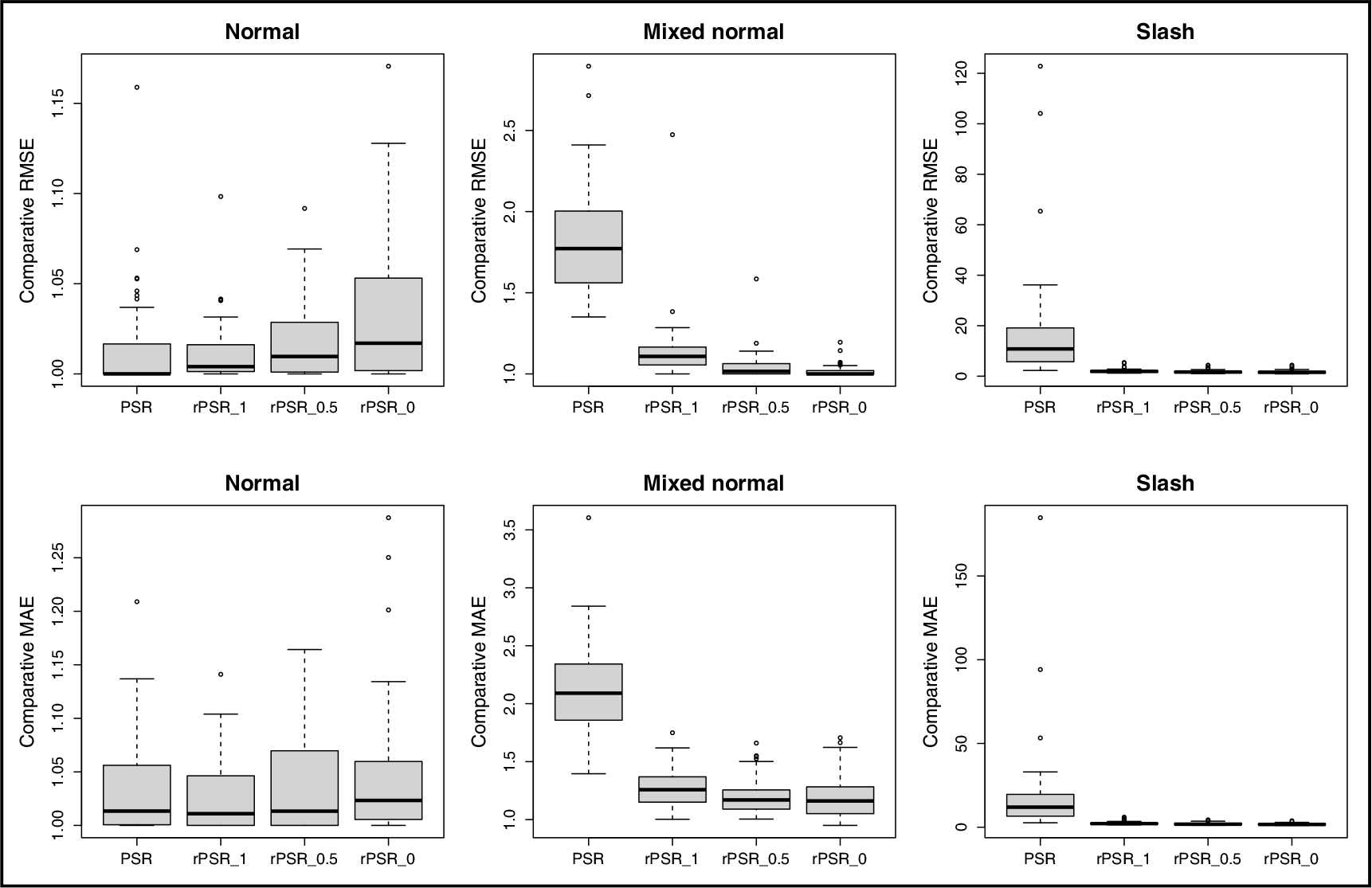
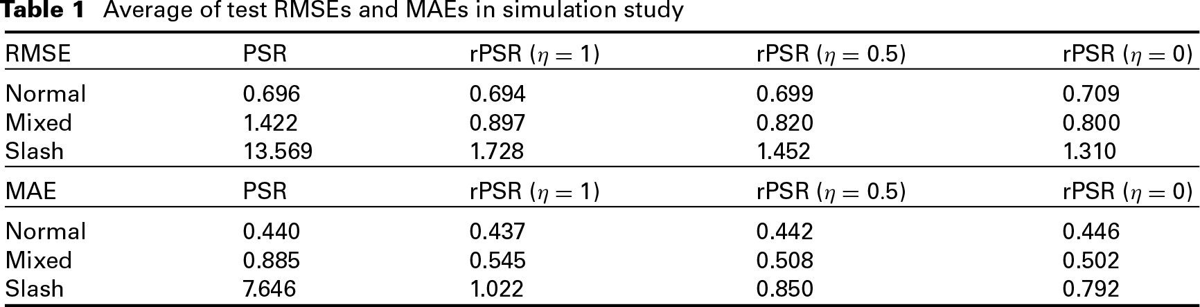
c_{i, j} = \frac{d_{ij}}{\min {d_{i, l}}_{l = 1, \dots, 4}}, i = 1, \dots, 50, j = 1, 2, 3, 4

where $d_{ij}$ is a performance measure (e.g., RMSE and MAE) over 50 replications for each of the four methods: PSR and rPSR with $η = 1$ , $0.5$ and $0$ . This quantity facilitates individual comparisons by using the test error of the best method for each dataset to calibrate the difficulty of the problem. Figure 5 shows the boxplots of the comparative RMSEs and MAE for PSR and rPSR based on 50 random replications. Table 1 shows the average of test RMSEs and MAEs based on 50 replications.

Figure 5:

Boxplots of comparative RMSE for rPSR and PSR under three error distributions

Table 1:

Average of test RMSEs and MAEs in simulation study

RMSE	PSR	rPSR ( $η = 1$ )	rPSR ( $η = 0.5$ )	rPSR ( $η = 0$ )
Normal	0.696	0.694	0.699	0.709
Mixed	1.422	0.897	0.820	0.800
Slash	13.569	1.728	1.452	1.310
MAE	PSR	rPSR ( $η = 1$ )	rPSR ( $η = 0.5$ )	rPSR ( $η = 0$ )
Normal	0.440	0.437	0.442	0.446
Mixed	0.885	0.545	0.508	0.502
Slash	7.646	1.022	0.850	0.792

Based on Figure 5 and Table 1, we have the following remarks: (a) For the normal error case, all three rPSR models have very close prediction performance with their competitor PSR. In fact, rPSR with Huber loss (i.e., $η = 1$ ) performs slightly better than PSR; (b) For the mixed case, all three rPSR methods perform substantially better than PSR. In particular, the rPSR models with $η = 0$ and 1 perform better than rPSR with Huber loss; (c) For the slash distribution case, PSR performs much worse than all three rPSR models. In some extreme case, PSR performs about 100 times worse than rPSR. Among the three rPSR models, rPSR with truncated least-square loss ( $η = 0$ ) performs the best.

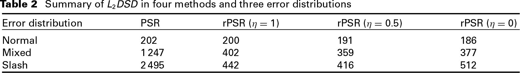
Model stability is an important issue in regression analysis. Generally, it is desired to have a stable estimate of regression coefficients and prediction on new data points. We consider the same three error distributions as above. For each error distribution, we randomly sample 95% of the data points (i.e., 641 out of 675), upon which the PSR and rPSR models (i.e., $η = 0$ , $0.5$ and $1$ ) with $λ = 10^{- 5}$ are fitted. To compare the model stability on regression coefficients, we use the $L_{2}$ distance standard deviation ( $L_{2} DSD$ ) criterion, defined by

L_{2} DSD = StDev ({| | {\hat{β}}^{(i)} - \bar{β} | |_{2}}_{i = 1}^{20}),

where $\bar{β}$ is the average regression coefficient vector based on 20 random replications. Note that $β$ is the regression coefficient vector on the wavelength, not on the basis functions, and $| | {\hat{β}}^{(i)} - \bar{β} | |$ is the Euclidean distance between the $i th$ estimate of $β$ and the average of the estimate over 20 trials. Table 2 shows the values of $L_{2} DSD$ for each method under different scenarios. We see that under the normal case, the variation of the regression coefficients on four methods is very close to each other. But PSR has much higher variation on regression coefficients in mixed and slash cases, where error distributions are heavily tailed.

Table 2:

Summary of $L_{2} DSD$ in four methods and three error distributions

Error distribution	PSR	rPSR ( $η = 1$ )	rPSR ( $η = 0.5$ )	rPSR ( $η = 0$ )
Normal	202	200	191	186
Mixed	1 247	402	359	377
Slash	2 495	442	416	512

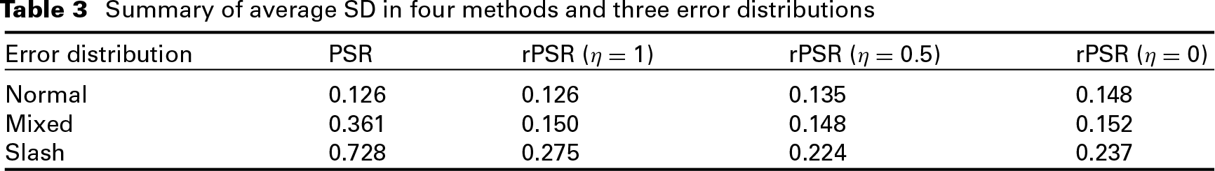
To evaluate the model stability on prediction, we use each of the 20 models (for each method and error distribution) to predict all 675 observations in the dataset. The SD of the predicted values on each observation was then calculated. The average of these 675 SDs are used to evaluate the model's consistency on prediction under data perturbation (i.e., resample 95% of the data). Table 3 shows the average SD for each method under different scenarios. We see that under normal errors, all four methods have close variation on prediction. However, in mixed normal and slash cases, PSR has much higher variation on prediction than the rPSR method.

Table 3:

Summary of average SD in four methods and three error distributions

Error distribution	PSR	rPSR ( $η = 1$ )	rPSR ( $η = 0.5$ )	rPSR ( $η = 0$ )
Normal	0.126	0.126	0.135	0.148
Mixed	0.361	0.150	0.148	0.152
Slash	0.728	0.275	0.224	0.237

5.2 Soil data results

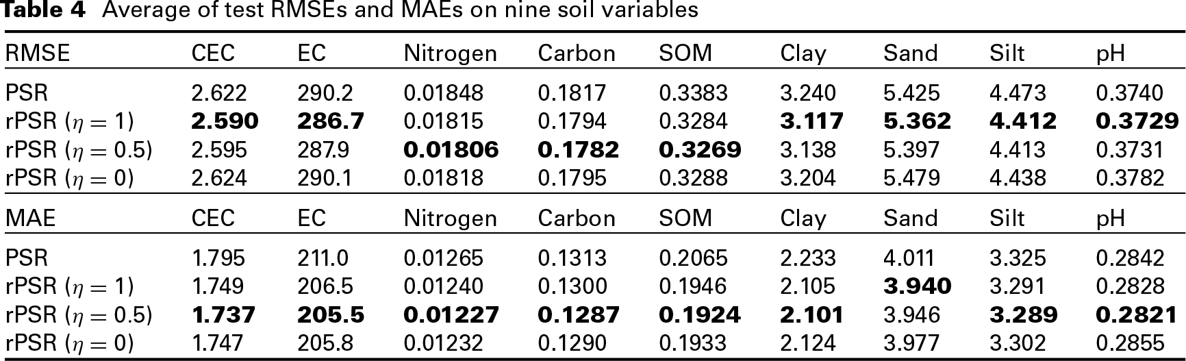
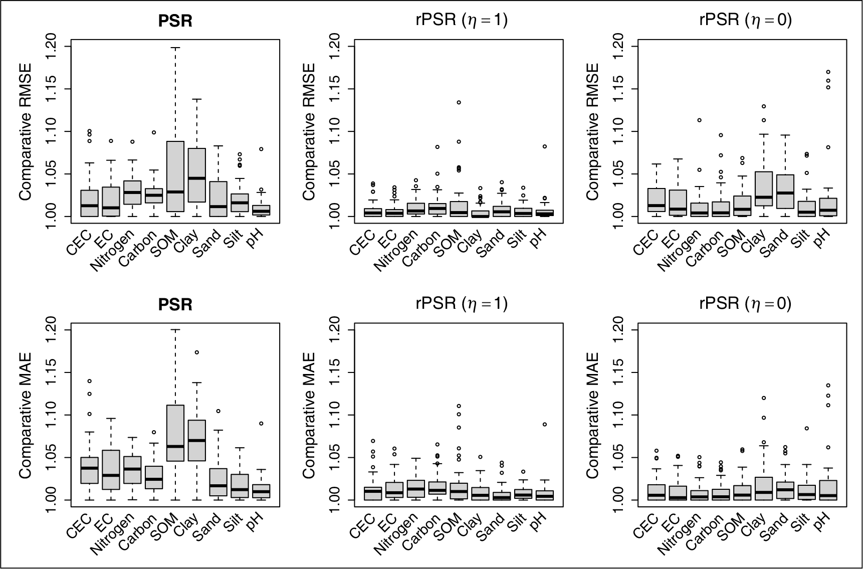
As with the simulation study, we randomly split the dataset into a training (sample size is 506) and a test set (the remaining 169 observations). PSR and rPSR with $η = 1$ , $0.5$ and $0$ are fitted on the training set and predict the test samples for all nine soil variables. Figure 6 shows the boxplots of comparative RMSE and MAE between rPSR (with $η = 1$ and $0$ ) and PSR on nine soil variables. Table 4 shows the average test RMSE and MAE of PSR and rPSR on nine soil variables, and highlights the best result in each column. The results are based on 50 random splits of the dataset. From Figure 6 and Table 4, we see that rPSR achieves better overall performance than PSR. In general, rPSR with Huber loss performs the best in RMSE and rPSR with $η = 0.5$ performs the best in MAE.

Table 4:

Average of test RMSEs and MAEs on nine soil variables

RMSE	CEC	EC	Nitrogen	Carbon	SOM	Clay	Sand	Silt	pH
PSR	2.622	290.2	0.01848	0.1817	0.3383	3.240	5.425	4.473	0.3740
rPSR ( $η = 1$ )	2.590	286.7	0.01815	0.1794	0.3284	3.117	5.362	4.412	0.3729
rPSR ( $η = 0.5$ )	2.595	287.9	0.01806	0.1782	0.3269	3.138	5.397	4.413	0.3731
rPSR ( $η = 0$ )	2.624	290.1	0.01818	0.1795	0.3288	3.204	5.479	4.438	0.3782
MAE	CEC	EC	Nitrogen	Carbon	SOM	Clay	Sand	Silt	pH
PSR	1.795	211.0	0.01265	0.1313	0.2065	2.233	4.011	3.325	0.2842
rPSR ( $η = 1$ )	1.749	206.5	0.01240	0.1300	0.1946	2.105	3.940	3.291	0.2828
rPSR ( $η = 0.5$ )	1.737	205.5	0.01227	0.1287	0.1924	2.101	3.946	3.289	0.2821
rPSR ( $η = 0$ )	1.747	205.8	0.01232	0.1290	0.1933	2.124	3.977	3.302	0.2855

Figure 6:

Boxplots of comparative RMSE and MAE for rPSR and PSR on nine responses

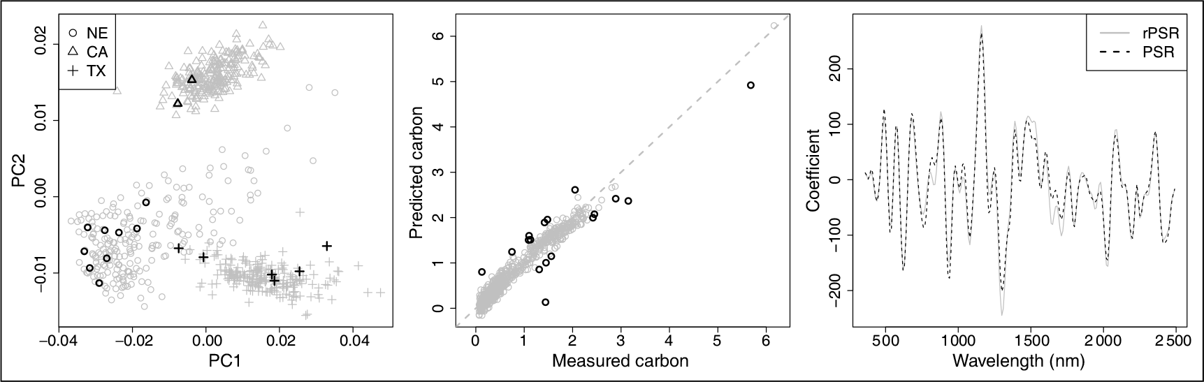
In order to see the identified outlying samples in the rPSR model and compare the coefficients between PSR and rPSR model, the PSR and rPSR model with $η = 0.5$ are fitted on all 675 spectra samples using carbon as the response variable. Since we already have a profile of optimal $λ$ values using CV based on 50 replications in the previous study, the median is used for rPSR and PSR models to fit all the samples. Figure 7 shows the PCA plot of all 675 spectra samples on the leading two principal components, which explain 79.8% of the total variance. Different symbols are used to distinguish the three sample locations: Nebraska, California and Texas. The highlighted symbols are the samples identified as outliers in the rPSR model. The rPSR model identified 17 outliers, which is about 2.5% of the total sample size. We see that the majority of the outlying samples are from Nebraska and Texas. We did not see any obvious pattern for the outliers in the PCA plot. The middle panel shows the prediction plot for the rPSR model. We see that the outliers are evenly distributed above and below the 45 degree line. Interestingly, although there are two samples on the right end of the plot, only one of them is an outlier. The right panel shows the coefficient curves for the rPSR and PSR models. The coefficients of two models are close to each other. Overall, the coefficient curve of rPSR model is slightly smoother than PSR model.

Figure 7:

PCA plot (left) of 675 samples from 3 locations with different symbols. The highlighted black points are the identified outliers from the rPSR model. The prediction plot (middle) with highlighted outliers (black). The coefficient plot (right) for rPSR (grey solid) and PSR (black dash) models.

6 Related issues

Two related issues are discussed in this section: computational efficiency of the rPSR algorithm and the $η$ effect in rPSR model.

6.1 Computation in rPSR

Computational efficiency is an important property of an algorithm. To examine the computational efficiency for the rPSR algorithm, we repeatedly applied rPSR ( $η = 1$ ) and PSR on the soil dataset ( $m = 675$ and $p = 214$ ) with CEC as the response variable 1 000 times. For each trial, the tuning parameter $λ$ was randomly chosen (i.e., ${log}_{10} λ \sim U (- 8, 5)$ ), and used for both rPSR and PSR. Both PSR and rPSR are in R. All the computing and timings were carried out on a computer node with two 10-core 2.8 GHz E5-2680v2 Xeon processors on Louisiana Optical Network Infrastructure (LONI) HPC systems.

Table 5 shows the total CPU timings of PSR and rPSR on 1 000 trials. For PSR, two computing modes are used: PSR $^{i}$ is the ‘inference’ mode of PSR using the signal.fit function from Marx and Eilers (1999); and PSR $^{s}$ is the ‘search’ mode of PSR. The signal.fit program, available at http://statweb.lsu., fits the PSR on multivariate calibration problems under the generalized linear model (GLM) framework. The signal.fit function outputs not only the fitted regression coefficients and predicted values on test samples but also provides a variety of useful model inference statistics and plots. However, we found the PSR $^{s}$ is more computationally efficient than PSR $^{i}$ . In addition, we see rPSR computes 1 000 trials within 7 seconds, which implies rPSR is computationally efficient and well suited for large datasets. The main difference between PSR $^{i}$ and PSR $^{s}$ algorithms are: (a) the latter fits several PSR models with different values of $λ$ in a batch, while the former fits the PSR model on one $λ$ each time. Hence, PSR $^{s}$ avoids unnecessarily recomputing several matrix multiplications in PSR fitting, for example, matrix products: $U = XB$ , $U^{'} U$ , $D^{'} D$ ; (b) PSR $^{s}$ does not provide the model inference and plots. The timing results in Table 5 indicate that in model selection and cross-validation procedure, using search mode of PSR is highly recommended. After model selection, the final model should be fitted using the inference mode of PSR.

An important factor related to the computational efficiency for the rPSR algorithm is the number of iterations in Step 2. For the above timing study, we also examined the number of iterations for the rPSR algorithm. The five number summary for the number of iterations among 1 000 trials are 7 (minimum), 9 (the first quartile, $Q_{1}$ ), 13 (median), 16 ( $Q_{3}$ ) and 26 (maximum). We find that although the rPSR algorithm averages approximately 13 iterations, the CPU timing for rPSR is shorter by 5 times to that of PSR. Note that the rPSR comparisons are honest in that they also included the initial PSR solution of $\hat{α}$ for Step 2.

Table 5:

CPU timings (in seconds) on PSR and rPSR

	PSR $^{i}$	PSR $^{s}$	rPSR
CPU times	28.6	1.44	6.55

6.2 The

η

effect in rPSR

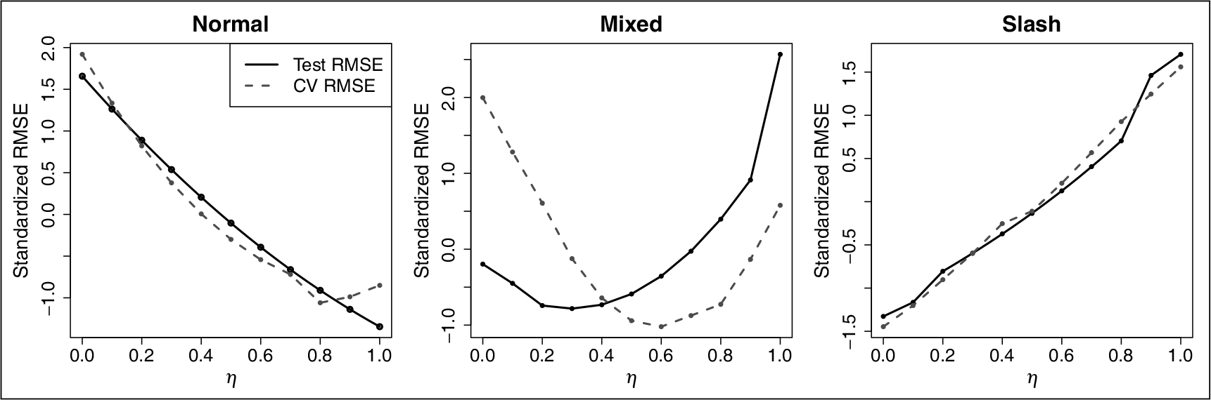
In generalized Huber criterion, there are two parameters: $K$ and $η$ . We have an automatic way to select the value of $K$ adapted to the data, described in Section 4.3. For $η$ , we can find the optimal value of $η$ through a grid search. The reason for using generalized Huber criterion rather than the Huber criterion is that the former provides more flexibility on down-weighting the outliers in errors than the latter. In particular, for datasets that are subject to extreme outlying residual, which are commonly encountered in practice, rPSR can adaptively use more robust loss function ( $η < 1$ ) than the Huber criterion ( $η = 1$ ). This is partially shown in the simulation study on three types of error distributions. For illustration, we additionally investigated the $η$ ‘effect’ based on a random split of the dataset as in the simulation study. We searched the optimal values of $λ$ and $η$ on a two-dimensional grid by minimizing the tenfold CV error on the training set. Figure 8 shows the standardized tenfold CV RMSE curve (dash) and test RMSE curve (solid) against $η$ on three types of error distribution. From the figure, we see the rPSR using Huber loss ( $η = 1$ ) performs the best when errors are normally distributed. For mixed normal errors, the optimal value of $η$ lies between 0 and 1. For slash distributed errors, the rPSR using the truncated least-square criterion ( $η = 0$ ) performs the best.

Figure 8:

Standardized cross-validation RMSE and test RMSE against different values of $η$ on three types of error distribution

6.3 Connection with Lee and Oh's (2007) procedure

Robust penalized regression spline was explored by Lee and Oh (2007), in which Huber loss was used. In Lee and Oh (2007), they proposed an iterative fitting procedure based on the ‘pseudo-response’:

{\tilde{y}}_{i} = {\hat{y}}_{i} + \frac{ψ (e_{i})}{2},

where $ψ (\cdot)$ is the first order derivative of Huber loss $ρ_{H} (\cdot)$ . We can show that the derivative of Huber loss is

ψ = 2 e_{i} - 2 I (| e_{i} | > K) [e_{i} - K Sign (e_{i})] .

As a result, the pseudo-response ${\tilde{y}}_{i}$ is equivalent to

{\tilde{y}}_{i} = y_{i} - I (| e_{i} | > K) [e_{i} - K Sign (e_{i})] .

(6.1)

From Equation (6.1), we can see that the pseudo-response in Lee and Oh's approach is a special case in adjusted response $Y^{A}$ described in (4.11) with $η = 1$ . However, Lee and Oh's approach is theoretically supported by Cox's result (Cox, 1983; Theorem 3.1 on pp. 536–537), while our approach is motivated by the d.c. programming in An and Tao (1997). In fact, Cox's Theorem 3.1 requires $ψ (\cdot)$ to be continuously differentiable up to the second order derivative, (i.e., $ψ \in C^{2} (- \infty, + \infty)$ ). However, the proposed generalized Huber criterion $ρ_{η} (\cdot)$ is not differentiable at $K$ and $- K$ . Compared with Lee and Oh's procedure, our proposed procedure is more general and motivated from a different perspective.

7 Discussion and future research

Although research had existed related to robust smoothing techniques, we did not find any research relating robust techniques to PSR or to the multicalibration problem. Not only is our proposed rPSR approach effective but it is also fast and simple to implement, effectively becoming an iterative PSR approach on an adjusted response. Some supplemental attractive features of our rPSR approach surface are: (a) There is no black box; the entire signal can be used as regressors; (b) As the precision of the signal increases ( $p$ grows), then the size of iterative system of equations remains unchanged and very manageable; (c) Since the estimated coefficient is smooth and spans over the entire index of the signal, potentially important regions can be visually identified; (d) Although we do not pursue it here, the rPSR approach can be transplanted into the GLM (e.g., the binary or Poisson response) framework; (e) More generally, rPSR extensions could be developed to accommodate multidimensional signal regression (Marx and Eilers, 2005), for example, where the signal is a two-dimensional surface or image; (f) Other future research could include a single index rPSR model, where $f (μ) = U α,$ for an explicit but unknown link function $f$ , along the lines of work found in Eilers et al. (2009) and Marx et al. (2011) for one- and two-dimensional signals, respectively.

Like other penalized methods, tuning parameter selection is critical in PSR. In this article, the optimal value of $λ$ is chosen to minimize the cross-validation RMSE. Ronchetti et al. (1997) proposed a robust cross-validation criterion, which is a weighted mean squared error, in robust linear model selection. Cantoni and Ronchetti (2001) extra and Tharmaratnam et al. (2010) introduced this robust cross-validation criterion into the robust smoothing splines. The main idea of using the robust cross-validation criterion is to down-weight the impact of the outlying points in the weighted predictive mean squared error. In our future work, we will implement and investigate the robust selection techniques in multivariate calibration problems.

Acknowledgments

The authors would like to thank the editor, associate editor and the referee for pointing out details that led to the connection and generalization of Lee and Ohs work, as well as for other constructive comments that helped to improve the scope of the article.

Declaration of Conflicting Interests

The author(s) declared no potential conflicts of interest with respect to the research, authorship and/or publication of this article.

Funding

The author(s) received no financial support for the research, authorship and/or publication of this article.

References

Tao

(1997) Solving a class of linearly constrained indefinite quadratic problems by d.c. algorithms. Journal of Global Optimization , 11, 253–285.

Cantoni

Ronchetti

(2001) Resistant selection of the smoothing parameter for smoothing splines. Statistics and Compu- ting , 11, 141–146.

Cox

(1983) Asymptotics for M-type smoothing splines. The Annals of Statistics , 11, 530–551.

Eilers

Menezes de

(2005) Quantile smoothing of array CGH data. Bioinfor- matics , 21, 1146–1153.

Eilers

Marx

(1996) Flexible smoothing with B-splines and penalties (with comments and rejoinder). Statistical Science , 11, 89–121.

Eilers

Marx

(2009) Multivariate calibration with single-index signal regre- ssion. Chemometrics and Intelligent Labo- ratory Systems , 96, 196–202.

Hall

Jones

(1990) Adaptive M-estimation in nonparametric regression. The Annals of Statistics , 18, 1712–1728.

Hrdle

Gasser

(1984) Robust non-para- metric function fitting. Journal of the Royal Statistical Society, Series B , 46, 42–51.

Simpson

Wang

(2000) Breakdown points of t-type regression estimators. Biometrika , 87, 675–1687.

10.

Huber

(1964) Robust estimation of a location parameter. The Annals of Mathematical Statistics , 35, 73–101.

11.

Huber

(1979) Robust smoothing. In Robustness in Statistics , edited by Launer

Wilkinson

pages 33–47. New York, NY: Academic Press.

12.

Huber

(1981) Robust Statistics . New York, NY: John-Wiley and Sons.

13.

Kneib

(2013) Beyond mean regression (with discussion). Statistical Modelling , 13, 275–303.

14.

Lee

(2007) Robust penalized regression spline fitting with application to additive mixed modeling. Computational Statistics , 22, 159–171.

15.

(2009) Robust and sparse bridge regression. Statistics and Its Interface , 2, 481–491.

16.

Maronna

Martin

Yohai

(2006) Robust Statistics: Theory and Methods . New York, NY: Wiley.

17.

Marx

Eilers

(1999) Generalized linear regression on sampled signals and curves: A P-spline approach. Technometrics , 41, 1–13.

18.

Marx

Eilers

(2005) Multidimensional penalized signal regression. Technometrics , 47, 13–22.

19.

Marx

Eilers

(2011) Multidimen- sional single-index signal regression. Che- mometrics and Intelligent Laboratory Systems , 109, 120–130.

20.

Randal

(2008) A reinvestigation of robust scale estimation in finite samples. Computational Statistics and Data Analysis , 52, 5014–5021.

21.

Ronchetti

Field

Blanchard

(1997) A robust linear model selection by cross-validation. Journal of the American Statistical Association , 92, 1017–1023.

22.

Rousseeuw

Croux

(1993) Alternatives to the median absolute deviation. Journal of the American Statistical Association , 88, 1273–1283.

23.

Rousseeuw

Hubert

(2011) Robust statistics for outlier detection. WIREs: Data Mining and Knowledge Discovery , 1, 73–79.

24.

Silverman

(1985) Some aspects of the spline smoothing approach to nonparametric regression curve fitting. Journal of the Royal Statistical Society, Series B , 47, 1–52.

25.

Tharmaratnam

Claeskens

Croux

Salibin-Barrera

(2010) S-estimation for penalized regression splines. Journal of Computational and Graphical Statistics , 19, 609–625.

26.

Wang

Chakraborty

Weindorf

Sharma

Paul

Ali

(2015) Synthesized use of VisNIR DRS and PXRF for soil characterization: Total carbon and total nitrogen. Geoderma,243–44, 157–167.

Multivariate calibration with robust signal regression

Abstract

Keywords

1 Introduction

2 The motivating example

Figure 1:

Thirty sample (first derivative) spectra for the soil data

The normal quantile-quantile plots of the residuals for nine response variables after fitting penalized signal regression using P-splines

4.1 Generalized Huber loss

5.1 Simulation studies

Boxplots of comparative RMSE for rPSR and PSR under three error distributions

Average of test RMSEs and MAEs in simulation study

Summary of L 2 DSD in four methods and three error distributions

Summary of average SD in four methods and three error distributions

Table 4:

Average of test RMSEs and MAEs on nine soil variables

Boxplots of comparative RMSE and MAE for rPSR and PSR on nine responses

PCA plot (left) of 675 samples from 3 locations with different symbols. The highlighted black points are the identified outliers from the rPSR model. The prediction plot (middle) with highlighted outliers (black). The coefficient plot (right) for rPSR (grey solid) and PSR (black dash) models.

6.1 Computation in rPSR

Table 5:

CPU timings (in seconds) on PSR and rPSR

Figure 8:

Standardized cross-validation RMSE and test RMSE against different values of η on three types of error distribution

Acknowledgments

Declaration of Conflicting Interests

Funding

References

Summary of $L_{2} DSD$ in four methods and three error distributions

Standardized cross-validation RMSE and test RMSE against different values of $η$ on three types of error distribution