Flexible quasi-beta regression models for continuous bounded data

1 Introduction

For the analysis of continuous bounded data, the simplex (Kieschnick and McCullough, 2003) and beta (Ferrari and Cribari-Neto, 2004) regression models are two frequent approaches. Both models are based on the principles of generalized linear models (Nelder and Wedderburn, 1972), relating the expected value of the response variable to covariates through a suitable link function. Such approaches are nowadays easily employed for practitioners, mainly because of the well-developed simplexreg (Zhang et al., 2016) and betareg (Cribari-Neto and Zeileis, 2010) packages for the statistical software R (R Development Core Team, 2017).

The literature on the analysis of continuous bounded data in the form of rates and proportions is rich. Standard simplex and beta regression models for independent data were presented in Ferrari and Cribari-Neto (2004), Kieschnick and McCullough (2003) and Paolino (2001) to cite but a few. Simas et al. (2010), Cepeda and Gamerman (2005) and Cepeda (2001) extend the beta regression model by regressing both mean and dispersion parameters on potential covariates. A similar extension has been done for simplex regression models in Song et al. (2004).

For the analysis of longitudinal and repeated measures data, Bonat et al. (2015a); Figueroa-Zúñiga et al. (2013) presented beta mixed models within the Bayesian paradigm. Bonat et al. (2015b) proposed a similar model class, in a pure likelihood framework. Similarly, Qiu et al. (2008) discussed the specification of simplex mixed models for longitudinal data, while a marginal version of the simplex model for modelling longitudinal data was proposed in Song and Tan (2000). Time series models for continuous bounded data were presented in Rocha and Cribari-Neto (2008), Grunwald et al. (1993) and McKenzie (1985). Influence and residuals analysis for beta regression models were discussed in Rocha and Simas (2011), Espinheira et al. (2008b) and (Espinheira et al. (2008a). Dynamic beta regression models were proposed by (da Silva et al. (2011). For further discussions and references on beta regression models see Smithson and Verkuilen (2006) and Verkuilen and Smithson (2012).

Additionally, new classes of probability density functions have been proposed for modelling continuous bounded data. Lemonte and Bazàn (2016) proposed a new class of Johnson S B distribution and associated regression models. Abdel-Fattah et al. (2016) presented a gamma regression model for bounded continuous response variables. Regression models based on the Kumaraswamy distribution has been proposed as an alternative to the beta regression model (Mitnik and Baek, 2013). Meanwhile, Kotz and van Dorp (2004) present many alternative probability density functions with bounded support.

Estimation and inference for regression models are generally done based on the standard method of maximum likelihood, which in turn provides efficient estimation for both regression and dispersion parameters. Although of broad use and efficient, the method of maximum likelihood requires a full model specification, that is, we need to specify a probability density function as the data generator. Given the plethora of available approaches to model continuous bounded data in the literature, it is difficult to decide, with conviction, which is the best choice for a particular dataset. The standard approach seems to take a small set of models, such as the beta, simplex, Kumaraswamy, etc. fit all of them and then choose the best fit by using some measures of goodness-of-fit, such as the Akaike or Bayesian information criteria. A typical example of this approach can be found in Bonat et al. (2012), where the authors compared the fit of four different distributions for the analysis of four datasets.

Although reasonable, such an approach is challenging to implement in practical data analysis. First, we should define the set of models to be fitted. Second, each bounded model can require specific fitting algorithms and give its own set of fitting problems, in general due to difficult aspects of the likelihood function. Third, the choice of the best fit may not be obvious, with different information criteria leading to different selected models. Finally, the uncertainty around the choice of the distribution is not taken into account when choosing the best fit. Thus, we claim that it is very useful and attractive to have a unified model that can automatically adapt to the underlying bounded data distribution and that can be easily implemented in practice.

The main goal of this article is to propose a new class of regression models for continuous bounded data. The proposed flexible quasi-beta regression model is based on second-moment assumptions, only. The expectation is modelled in the orthodox way by means of a link function and a linear predictor. The variance is specified by ϕ μ p ( 1 − μ ) p , where μ is the mean and ϕ is the dispersion parameter. Finally, the extra power parameter p is introduced to give more flexibility in the modelling of the mean and variance relationship. As we shall show in Section 2, such a mean and variance relationship is often found in bounded distributions, which implies that the proposed model can easily mimic many well-known regression models, such as the beta and simplex regression models. Our approach for model specification resembles Wedderburn's quasi-likelihood (Wedderburn, 1974) method and has been recently used in the context of continuous and count data by Bonat and Kokonendji (2017) and Bonat et al. (2017), respectively. In this framework, we do not specify a full probability distribution for the bounded response variable and consequently a likelihood function is not available. Thus, the models are fitted by an estimating function approach as in in Bonat and Jørgensen (2016); Jørgensen and Knudsen (2004) obtained by combining the quasi-score and Pearson estimating functions for the estimation of the regression and dispersion parameters, respectively.

In the next section, we provide some background on regression models for continuous bounded data and present the flexible quasi-beta regression models. We focus on simplex and beta regression models because they are easily available in R. Section 3 discusses the estimating function approach employed for estimation and inference. Section 4 presents the main results from our simulation study. In Section 5 we illustrate the application of the flexible quasi-beta regression model through the analysis of two datasets. Finally, Section 6 gives some final remarks. Datasets and R code are available in the supplementary material.

2 Regression models for continuous bounded data

In this section, we shall explore the mean and variance relationship induced by the simplex and beta distributions. Furthermore, we use it as motivation to propose a new class of regression models to deal with continuous bounded data based on second-moment assumptions.

Let Y ∼ S − ( μ , ϕ ) denote a simplex distributed random variable with probability density function given by

f ( y ; μ , ϕ ) = ( 2 π ϕ 2 { y ( 1 − y ) 3 } ) − 1 / 2 exp { − 1 2 ϕ 2 { ( y − μ ) 2 y ( 1 − y ) μ 2 ( 1 − μ ) 2 } } ,

(2.1)

where y , μ ∈ ( 0 , 1 ) and ϕ > 0 is a dispersion parameter.

J∅rgensen (1997) showed that E ( Y ) = μ and

var ( Y ) = μ ( 1 − μ ) − 1 2 ϕ 2 exp 1 2 ϕ 2 μ 2 ( 1 − μ ) 2 Γ 1 2 , 1 2 ϕ 2 μ 2 ( 1 − μ ) 2 .

We note in passing that var ( Y ) → μ ( 1 − μ ) for ϕ → ∞ , that is, the simplex mean and variance relationship corresponds to the Bernoulli mean and variance relationship.

Similarly, let Y ∼ B ( μ , ϕ ) denote a beta distributed random variable with probability density function as follows

f ( y ; μ , ϕ ) = Γ ( ϕ ) Γ ( μ ϕ ) Γ ( ( 1 − μ ) ϕ ) y μ ϕ − 1 ( 1 − y ) ( 1 − μ ) ϕ − 1 ,

(2.2)

where y , μ ∈ ( 0 , 1 ) and ϕ > 0 is now a precision parameter (inverse of dispersion). Ferrari and Cribari-Neto (2004) showed that E ( Y ) = μ and var ( Y ) = μ ( 1 − μ ) 1 + ϕ . Thus, it is easy to see that when ϕ → 0 , the var ( Y ) → μ ( 1 − μ ) , which in turn also corresponds to the mean and variance relationship of the Bernoulli distribution. Furthermore, for both simplex and beta distributions, the largest possible variance is 0.25 , and it is reached when μ = 0.5 for extreme values of ϕ .

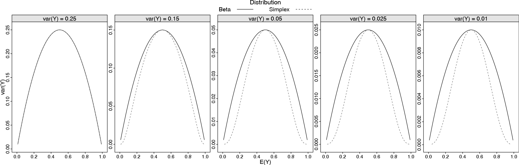
Figure 1 shows the mean and variance relationship of the simplex and beta distributions for different values of ϕ . We fixed the values of ϕ to have different levels of variance when μ = 0.5 . Thus, for var ( Y ) = 0.25 , 0.15 , 0.05 , 0.025 and 0.01 , the values of the simplex dispersion parameter were ϕ = 10 00 000, 9.1500, 2.4067, 1.4651, 0.8487, while for the beta distribution the precision parameter ϕ = 0.00001 , 0.6660 , 4 , 9 , 23.9989 .

OPEN IN VIEWER Figure 1

Mean and variance relationship beta and simplex distributions

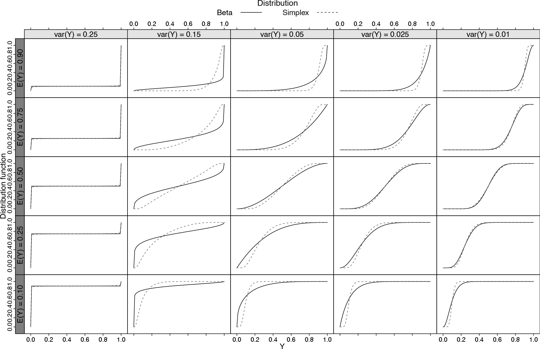
The mean and variance relationship shows that the main differences between the distribution shapes appear as μ moves away from 0.5 . In general, the beta tails are heavier than the simplex tails. To better illustrate these differences, Figure 2 presents the cumulative probability function of the simplex and beta distributions for different values of the expectation and variance of Y .

OPEN IN VIEWER Figure 2

Beta and simplex cumulative probability function by values of the variance (fixed for μ = 0.5 ) and expectation

The cumulative probability functions presented in Figure 2 highlight the flexibility of both distributions to deal with continuous bounded data. In the extreme case of var ( Y ) = 0.25 , both distributions present virtually the same mean and variance relationship and consequently very similar cumulative probability function (i.e., Bernoulli). For smaller variances the distributions are really similar for values of the mean around 0.5 , while quite different in the tails. Such results emphasize that in practice one distribution can fit better than the other for an observed dataset. Thus, a data analysis should consider both of these, or even other alternative distributions.

In spite of the differences in the mean and variance relationship between the simplex and beta distributions, such a relationship can be well modelled by a simple function of the expected values μ . This fact motivates us to specify a regression model by using only second-moment assumptions. Thus, consider a cross-sectional dataset, ( y i , x i ) , i = 1 , … , n , where y i s are independent and identically distributed realizations of Y i according to an unspecified distribution, whose expectation and variance are given by

E ( Y i ) = μ i = g − 1 ( x i ⊤ β ) var ( Y i ) = σ i = ϕ μ i p ( 1 − μ i ) p ,

(2.3)

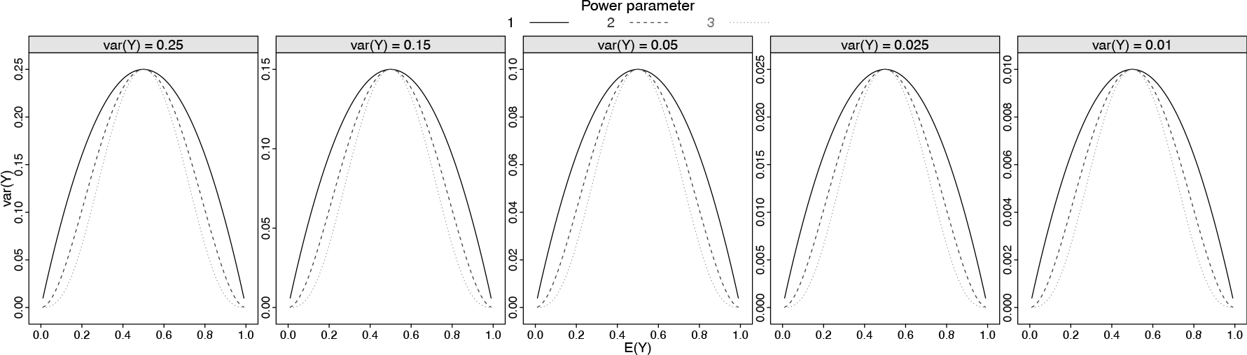
where x i and β are ( q × 1 ) vectors of known covariates and unknown regression parameters, respectively. Moreover, g is a standard link function, for which here we adopt the logit link function to give mean values in the interval ( 0 , 1 ) , but potentially any other suitable link function could be adopted. The regression model specified in (2.3) is parametrized by θ = ( β ⊤ , λ ⊤ ) ⊤ , where λ = ( ϕ , p ) with the usual parameter space and can mimic the mean and variance relationship of both simplex and beta models as shown in Figure 3.

OPEN IN VIEWER Figure 3

Mean and variance relationship modelled by the function var ( Y ) = ϕ μ p ( 1 − μ ) p by values of the var ( Y ) and power parameter p

As expected for p = 1 , our model corresponds to the beta regression model in a slightly different parametrization. The plots in Figure 3 show that the simplex mean and variance relationship is well approximated by using p = 3 when var ( Y ) ≤ 0.15 , although there is no direct equivalence with the simplex distribution. However, in practice, any simplex or beta distributions can be the best choice for a particular dataset. Thus, the algorithm we shall present in Section 3 allows us to estimate the power parameter, which in turn works as an automatic model selection. In this sense, the model proposed in (2.3) unifies the simplex and beta regression models and provides a broader class of regression models for continuous bounded data.

In this section, we present the estimating function approach used for fitting the flexible quasi-beta regression models using terminologies and results from Jørgensen and Knudsen (2004) and Bonat and Jørgensen (2016). We adopt the quasi-score and Pearson estimating functions for estimation of the regression and dispersion parameters, respectively. The quasi-score function for β is given by,

ψ β ( β , λ ) = ∑ i = 1 n ∂ μ i ∂ β 1 σ i − 1 ( Y i − μ i ) , … , ∑ i = 1 n ∂ μ i ∂ β q σ i − 1 ( Y i − μ i ) ⊤ ,

where ∂ μ i / ∂ β j = μ i ( 1 − μ i ) x ij for j = 1 , … , q .

The entry ( j , k ) of the q × q sensitivity matrix S β for ψ β is given by

S β jk = E ∂ ∂ β k ψ β j ( β , λ ) = − ∑ i = 1 n μ i ( 1 − μ i ) x ij σ i − 1 x ik μ i ( 1 − μ i ) .

(3.1)

In a similar way, the entry ( j , k ) of the q × q variability matrix V β for ψ β is given by

V β jk = Cov ( ψ β j ( β , λ ) , ψ β k ( β , λ ) ) = ∑ i = 1 n μ i ( 1 − μ i ) x ij σ i − 1 x ik μ i ( 1 − μ i ) .

The Pearson estimating functions for the dispersion parameters have the following form,

ψ λ ( λ , β ) = − ∑ i = 1 n ∂ σ i − 1 ∂ ϕ ( Y i − μ i ) 2 − σ i , − ∑ i = 1 n ∂ σ i − 1 ∂ p ( Y i − μ i ) 2 − σ i ⊤ .

It is important to highlight that the Pearson estimating functions are unbiased estimating functions for λ based on the squared residuals ( Y i − μ i ) 2 with expected value σ i .

The entry ( j , k ) of the 2 × 2 sensitivity matrix S λ for the dispersion parameters is given by

S λ jk = E ∂ ∂ λ k ψ λ j ( λ , β ) = − ∑ i = 1 n ∂ σ i − 1 ∂ λ j σ i ∂ σ i − 1 ∂ λ k σ i ,

(3.2)

where λ j and λ k denote either ϕ or p . The cross entries of the sensitivity matrices S β λ and S λ β are given by

S β j λ k = E ∂ ∂ λ k ψ β j ( β , λ ) = 0

(3.3)

and

S λ j β k = E ∂ ∂ β k ψ λ j ( λ , β ) = − ∑ i = 1 n ∂ σ i − 1 ∂ λ j σ i ∂ σ i − 1 ∂ β k σ i .

(3.4)

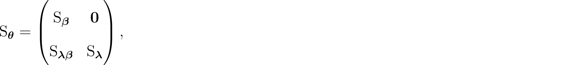
Finally, the joint sensitivity matrix for the parameter vector θ is given by

S θ = S β 0 S λ β S λ ,

whose entries are defined by equations (3.1), (3.2), (3.3) and (3.4).

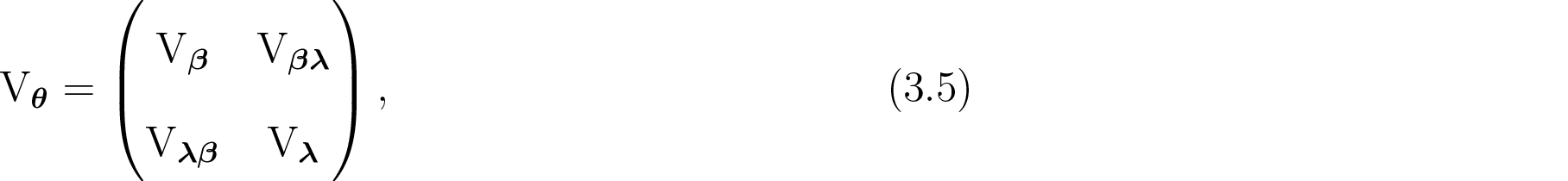
The asymptotic variance of the estimating function estimators denoted by θ ̂ is obtained from the inverse Godambe information matrix, whose general form for a vector parameter θ is J θ − 1 = S θ − 1 V θ S θ − ⊤ , where − ⊤ denotes inverse transpose. The variability matrix for θ has the form

V θ = V β V β λ V λ β V λ ,

(3.5)

where V λ β = V β λ ⊤ and V λ depend on the third and fourth moments of Y i , respectively. In order to avoid this dependence on higher-order moments, we adopt the approach proposed in Bonat and Jørgensen (2016) that consists of using the empirical versions of V λ and V λ β as given by

V ̃ λ jk = ∑ i = 1 n ψ λ j ( λ , β ) i ψ λ k ( λ , β ) i and V ̃ λ j β k = ∑ i = 1 n ψ λ j ( λ , β ) i ψ β k ( λ , β ) i .

Finally, the approximate distribution of θ ̂ Jørgensen and Knudsen, 2004; (Godambe and Thompson, 1978) is the multivariate Gaussian distribution with expectation θ and covariance matrix J θ − 1 = S θ − 1 V θ S θ − ⊤ .

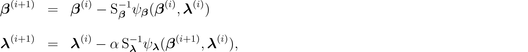
To solve the system of equations ψ β = 0 and ψ λ = 0 , we adopted the modified chaser algorithm proposed by Jørgensen and Knudsen (2004) and implemented in a very general form in the package mcglm (Bonat, 2018) for the statistical software R. The modified chaser algorithm uses the insensitivity property (3.3), which allows us to use two separate equations to update β and λ as follows

β ( i + 1 ) = β ( i ) − S β − 1 ψ β ( β ( i ) , λ ( i ) ) λ ( i + 1 ) = λ ( i ) − α S λ − 1 ψ λ ( β ( i + 1 ) , λ ( i ) ) ,

where α is a tuning constant used to control the step-length. This algorithm was used by Bonat and Kokonendji (2017); and Bonat et al. (2017) for estimation and inference in the context of Tweedie and Poisson–Tweedie regression models, respectively. Furthermore, this algorithm is a special case of the flexible algorithm presented by Bonat and Jørgensen (2016) in the context of multivariate covariance generalized linear models.

In this section, we present a simulation study conducted to verify the properties of the estimating function estimators. We designed five simulation scenarios to explore the flexibility of the proposed regression model to deal with bounded data, as generated from the simplex and beta distributions. For each setting, we considered five different sample sizes, 50 , 100 , 250 , 500 and 1 000 , generating 1 000 datasets in each case. The dispersion parameter of the simplex distribution was fixed at the values ϕ = 10 000 000 , 9.1500 , 2.4067 , 1.4651 , 0.8487 and the corresponding precision parameter for the beta distribution at ϕ = 0.00001 , 0.6660 , 4 , 9 , 23.9989 . These values correspond to var ( Y ) = 0.25 , 0.15 , 0.05 , 0.025 , 0.01 when μ = 0.5 . Thus, we can explore the behaviour of the fitting algorithm as well as the properties of the estimators from an extreme and challenging ( var ( Y ) = 0.25 ) to an easy ( var ( Y ) = 0.01 ) scenario.

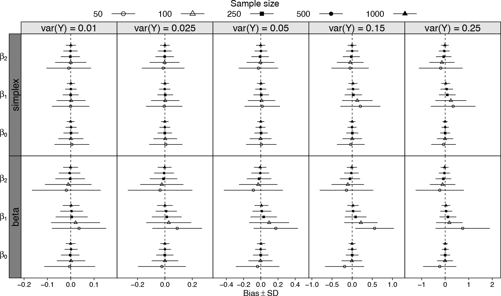
For all scenarios, we consider a standard regression model where the linear predictor is composed of a continuous and a categorical covariate. The continuous covariate was generated from a standard Gaussian distribution and the categorical covariate from a Bernoulli distribution with probability fixed at 0.5 . The regression coefficients were fixed at β 0 = 0 , β 1 = 3 for the continuous covariate, and β 2 = − 1.5 for the categorical indicator variable. Such values were chosen in order to cover the whole range of values for the expectation of the random variable, that is, the unit interval. Figure 4 shows the average bias plus and minus the average standard error for the regression parameter estimators under each scenario.

OPEN IN VIEWER

Figure 4

Average bias and confidence intervals by sample size and simulation scenario

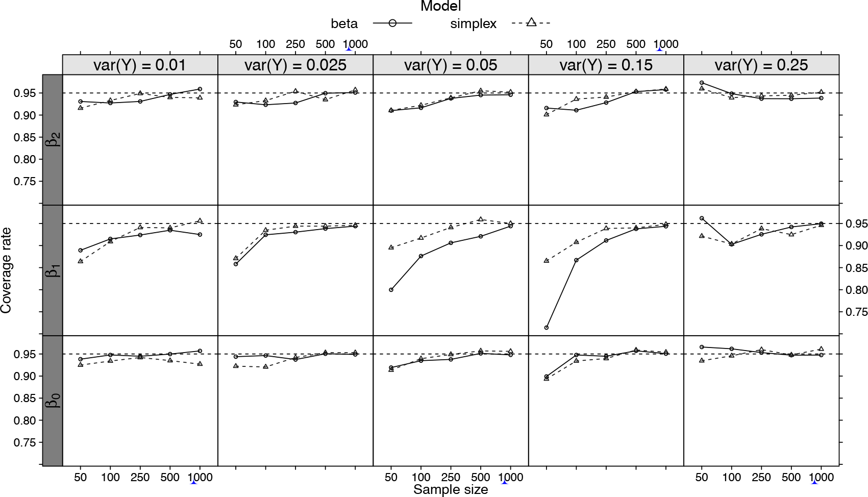
The results in Figure 4 show clearly that the bias and standard error (SE) of the estimating function estimators tend to zero as the sample size increases. Thus, we can conclude that the estimating function estimators are unbiased and consistent for large samples, as expected. For small sample sizes, the results in Figure 4 show that the bias tends to increase from the easy var ( Y ) = 0.01 to the challenging var ( Y ) = 0.25 scenario, again as expected. In general, the biases are larger when using the beta distribution than the simplex distribution as the data generator, mainly for the parameter β 1 . Figure 5 presents the coverage rate for the individual parameter confidence intervals by sample size and simulation scenario.

The results in Figure 5 show that the empirical coverage rates are close to the nominal level of 95 % for large samples. On the other hand, for small sample sizes and large variance scenarios the empirical coverage rate for the continuous covariate regression coefficient β 1 presented values around 80 % . This result shows that for these scenarios, the estimation of the standard errors associated with the regression coefficients is challenging and thus requires large samples for their correct estimation.

In this section, we illustrate the application of the flexible quasi-beta regression through the analysis of two datasets. The first dataset concerns measures of the water quality index collected at 16 hydroelectric power plants in Paraná State, Brazil. This dataset was analysed in Bonat et al. (2015a,b, 2018) using beta and simplex mixed models. Bonat et al. (2018) showed that the simplex distribution fits better than the beta distribution to this dataset. The second dataset corresponds to observations of the stress and anxiety indices among non-clinical women in Townsville, Queensland, Australia. This dataset is part of the betareg Cribari-Neto and Zeileis (2010) package and the beta distribution clearly fits better than the simplex distribution to this dataset. Thus, we have a case where the simplex fits better and another for which the beta distribution provides the better fit. Our goal is to show that the proposed model fits well for both cases. The datasets and the R scripts used for their analysis can be obtained http://www.leg.ufpr.br/doku.php/ publications:papercompanions:quasibeta.

OPEN IN VIEWER

Figure 5

Coverage rate for each regression parameter confidence interval by sample size and simulation scenario

5.1 Dataset 1: Water quality on power plant reservoirs

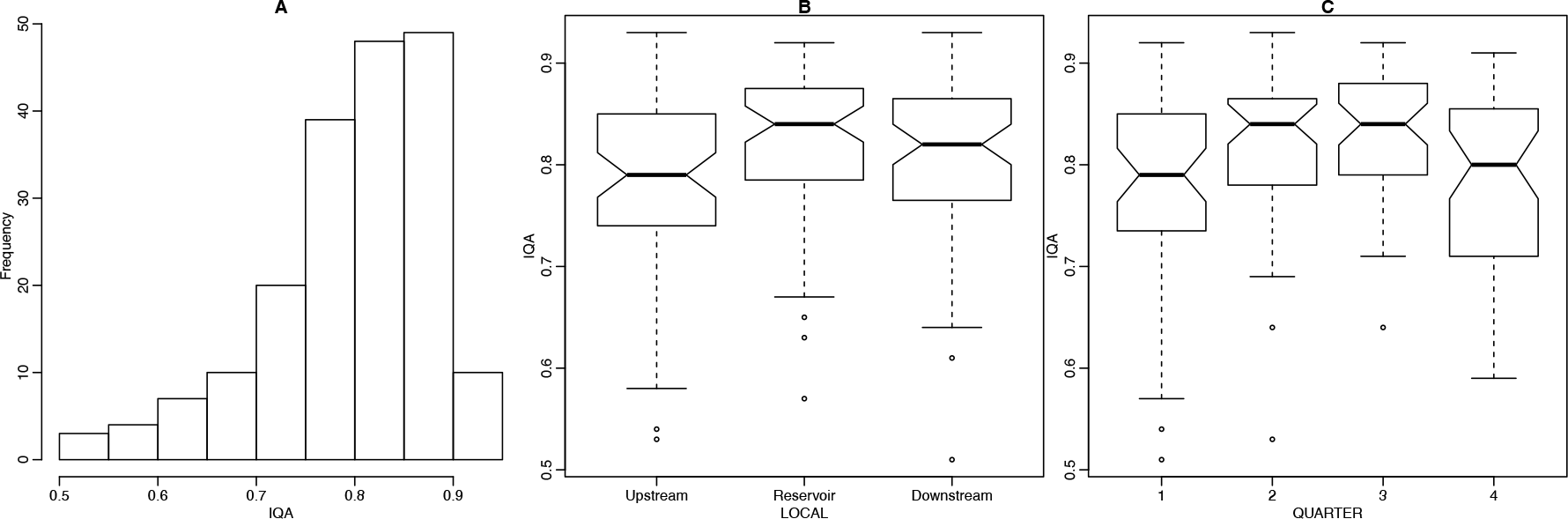
The water quality dataset corresponds to observations of the water quality index measured quarterly during 2004 at 16 operating hydroelectric power plants in Paraná State, Brazil. The main goal of this study was to detect changes in water quality, possibly due to the presence of the dams. The water quality index was measured at locations considered affected and unaffected by the reservoir and then compared, that is, measurements taken upstream in the main river are considered unaffected reference values, whereas measurements taken at the reservoir and downstream are considered potentially affected. Thus, the main goal is to assess the effect of the covariate LOCAL, with levels upstream, reservoir and downstream, controlled for the effects of the QUARTER of data collection. In this article, for simplicity, we do not consider the possible effect of the individual power plants. The dataset has 190 observations with 12 measurements ( 4 quarters × 3 locations) for each of the 16 power plants with only two missing values. Figure 6 presents a histogram and boxplots relating the response variable to the potential covariates.

OPEN IN VIEWER

Figure 6

Histrogram (A) and boxplots for the LOCAL(B) and QUARTER(C) for the water quality index (IQA)

Figure 6(A) shows a left asymmetry in the marginal distribution, while Figure 6(B) suggests that upstream observations present smaller values than reservoir and downstream. Furthermore, Figure 6(C) indicates that the water quality index presents smaller values on the first and fourth quarters (warmer periods).

We fitted the flexible quasi-beta regression model to the water quality dataset using a logit link function. The linear predictor is composed of the LOCAL and QUARTER covariates, that is,

η it = β 0 + β 1 i + β 2 t ,

(5.1)

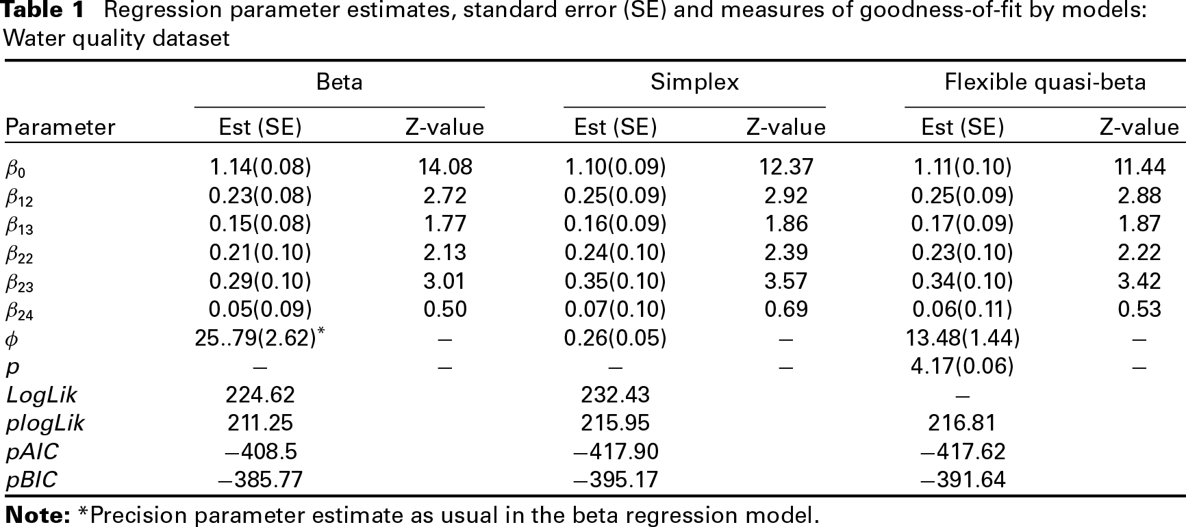
where β 0 is the usual intercept, and β 1 i , for i = 2 , 3 , measures the changes from upstream to reservoir and downstream, respectively. Similarly, β 2 t , for t = 2 , 3 and 4 , quantifies the changes from quarter 1 to 2 up to 4 , respectively. Table 1 shows the parameter estimates for the beta, simplex and the flexible quasi-beta regression models along with the maximized log-likelihood (beta and simplex) and pseudo-Gaussian log-likelihood values Bonat et al. (2018) and the associated pseudo Akaike and Bayesian information criteria.

OPEN IN VIEWER

Table 1

Regression parameter estimates, standard error (SE) and measures of goodness-of-fit by models: Water quality dataset

	Beta		Simplex		Flexible quasi-beta
Parameter	Est (SE)	Z-value	Est (SE)	Z-value	Est (SE)	Z-value
β 0	1.14 ( 0.08 )	14.08	1.10 ( 0.09 )	12.37	1.11 ( 0.10 )	11.44
β 12	0.23 ( 0.08 )	2.72	0.25 ( 0.09 )	2.92	0.25 ( 0.09 )	2.88
β 13	0.15 ( 0.08 )	1.77	0.16 ( 0.09 )	1.86	0.17 ( 0.09 )	1.87
β 22	0.21 ( 0.10 )	2.13	0.24 ( 0.10 )	2.39	0.23 ( 0.10 )	2.22
β 23	0.29 ( 0.10 )	3.01	0.35 ( 0.10 )	3.57	0.34 ( 0.10 )	3.42
β 24	0.05 ( 0.09 )	0.50	0.07 ( 0.10 )	0.69	0.06 ( 0.11 )	0.53
ϕ	25 . . 79 ( 2.62 ) *	−	0.26 ( 0.05 )	−	13.48 ( 1.44 )	−
p	−	−	−	−	4.17 ( 0.06 )	−
LogLik	224.62		232.43		−
plogLik	211.25		215.95		216.81
pAIC	− 408.5		− 417.90		− 417.62
pBIC	− 385.77		− 395.17		− 391.64

Note: *Precision parameter estimate as usual in the beta regression model.

The results presented in Table 1 show a large difference in terms of log-likelihood values in favour of the simplex regression model. In spite of such a large difference, both models provide very similar regression estimates and standard errors, leading to identical interpretations. Similarly, the pseudo log-likelihood, Akaike and Bayesian information criterion indicates that the simplex model provides a better fit than the beta model. The flexible quasi-beta model presents regression estimates and standard errors similar to both simplex and beta regression models. The power parameter estimate was p ̂ = 4.17 ( 0.06 ) showing that probably the beta distribution ( p = 1 ) is not the best choice for this water quality dataset. This result agrees with the log-likelihood criterion. Furthermore, the pseudo log-likelihood criterion indicates that the flexible quasi-beta model provides an even better fit than the simplex model. Such a result is expected, since the proposed model has a more flexible mean and variance relationship than the beta and simplex regression models and consequently can mimic the fit of the other two models. Note that, the use of information criterion to compare the quasi-beta with the beta and simplex models can be misleading because we have one more parameter in the flexible quasi-beta that is fixed when fitting the beta and simplex regression models.

5.2 Dataset 2: Stress anxiety dataset

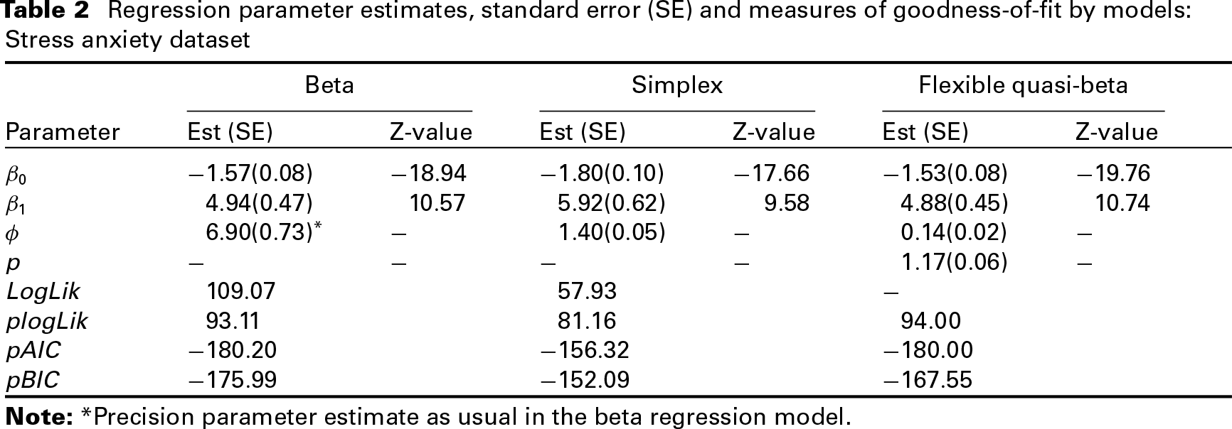
The second dataset concerns an experiment conducted to assess the relationship between stress and anxiety. Both variables were assessed through the Depression Anxiety Stress Scales, with scores ranging from 0 to 42 . Subsequently, they were linearly transformed to the open unit interval, for details see Smithson and Verkuilen (2006). The main goal of the analysis is to assess the effect of the anxiety score on the response variable stress score. We fitted the beta, simplex and flexible quasi-beta regression models, where the linear predictor is composed of an intercept ( β 0 ) and the effect of the covariate anxiety score ( β 1 ) , again using the standard logit link function. Table 2 shows the parameter estimates for the beta, simplex and the flexible quasi-beta regression models along with the maximized log-likelihood (beta and simplex) and pseudo-Gaussian log-likelihood values and the associated pseudo Akaike and Bayesian information criteria.

OPEN IN VIEWER

Table 2

Regression parameter estimates, standard error (SE) and measures of goodness-of-fit by models: Stress anxiety dataset

	Beta		Simplex		Flexible quasi-beta
Parameter	Est (SE)	Z-value	Est (SE)	Z-value	Est (SE)	Z-value
β 0	− 1.57 ( 0.08 )	− 18.94	− 1.80 ( 0.10 )	− 17.66	− 1.53 ( 0.08 )	− 19.76
β 1	4.94 ( 0.47 )	10.57	5.92 ( 0.62 )	9.58	4.88 ( 0.45 )	10.74
ϕ	6.90 ( 0.73 ) *	−	1.40 ( 0.05 )	−	0.14 ( 0.02 )	−
p	−	−	−	−	1.17 ( 0.06 )	−
LogLik	109.07		57.93		−
plogLik	93.11		81.16		94.00
pAIC	− 180.20		− 156.32		− 180.00
pBIC	− 175.99		− 152.09		− 167.55

Note: *Precision parameter estimate as usual in the beta regression model.

Based on the log-likelihood criterion, the beta regression model provides a better fit than the simplex model for this stress anxiety dataset. The regression coefficient associated with the covariate anxiety score is approximately 20 % larger when fitting the simplex model. The pseudo log-likelihood criterion agrees with the log-likelihood criterion showing the better fit of the beta model. The fit of the flexible quasi-beta regression model also suggests that the beta regression is a suitable choice for this dataset. The estimated value of the power parameter p ̂ = 1.17 ( 0.06 ) indicates a mean and variance relationship close to that of the beta distribution. The regression coefficient obtained based on the beta and flexible quasi-beta regression models are quite similar. Finally, the pseudo log-likelihood criterion also indicates that the beta and the flexible quasi-beta regression models provide a very similar fit.

We described a new class of regression models to deal with continuous bounded data. Our approach is based on second-moment assumptions, where we extend the beta mean and variance relationship by the inclusion of an additional power parameter. Thus, the flexible quasi-beta regression model can automatically adapt to the unknown underlying bounded data distribution by the estimation of this power parameter. Furthermore, the second-moment assumptions allow us to use an estimating functions approach for parameter estimation and inference. The main technical advantage of the proposed models is the simplicity of the fitting algorithm, which amounts to finding the root of a set of non-linear equations.

We designed five simulation scenarios to explore and show the performance of our fitting algorithm. The simulation scenarios range from very easy var ( Y ) = 0.01 to extreme and challenging var ( Y ) = 0.25 scenarios. It is important to highlight that in the last scenario, the simulated values are numerically 0 s and 1 s only. Thus, standard implementations of the beta and simplex regression models fail for fitting the model in this case. On the other hand, the flexible quasi-beta regression model and the associated estimating function approach proposed for model fitting delivered approximately unbiased and consistent estimates for all simulation scenarios even for small sample sizes. Furthermore, the coverage rate of the obtained confidence intervals presented values close to the nominal level of 95 % for large samples.

We illustrated the application of the flexible quasi-beta regression models through the analysis of two datasets. The datasets were chosen to show a situation where the simplex regression model is better than the beta regression model and vice-versa. In the data analyses, the pseudo log-likelihood criterion assists us to indicate that the flexible quasi-beta regression model, proposed in this article, automatically adapted to the underlying data distribution, and in turn provides more reliable results even when the data distribution is unknown.

The basic model discussed in this article can be extended in many ways, including incorporating penalized splines and the use of regularization for high dimensional data, with important applications in covariate selection. We plan to develop improved methods for model checking, such as residual analysis, leverage and outlier detection. Finally, we can extend the model to deal with multiple bounded response variables, with important applications for the analysis of longitudinal and spatial data. These extensions will form the basis of future work.

Declaration of conflicting interests

The authors declared no potential conflicts of interest with respect to the research, authorship and/or publication of this article.

Funding

The last author was partially supported by CNPq, a Brazilian science funding agency.

Supplementary material

Supplementary material is available at: http://www.leg.ufpr.br/doku.php/publications:papercompanions:quasibeta