Spatio-temporal expectile regression models

Abstract

Spatio-temporal models are becoming increasingly popular in recent regression research. However, they usually rely on the assumption of a specific parametric distribution for the response and/or homoscedastic error terms. In this article, we propose to apply semiparametric expectile regression to model spatio-temporal effects beyond the mean. Besides the removal of the assumption of a specific distribution and homoscedasticity, with expectile regression the whole distribution of the response can be estimated. For the use of expectiles, we interpret them as weighted means and estimate them by established tools of (penalized) least squares regression. The spatio-temporal effect is set up as an interaction between time and space either based on trivariate tensor product P-splines or the tensor product of a Gaussian Markov random field and a univariate P-spline. Importantly, the model can easily be split up into main effects and interactions to facilitate interpretation. The method is presented along the analysis of spatio-temporal variation of temperatures in Germany from 1980 to 2014.

Keywords

expectile regression interaction terms main effects tensor product P-spline spatio- temporal model

1 Introduction

In many areas of applied sciences, longitudinal data are recorded at several locations and multiple time points. Simple statistical models then estimate the temporal and the spatial effects as additive components (see Fahrmeir et al., 2004). Hence, the impact of time and space is assumed to be independent of each other while, for example, variations of the spatial effect over time are not considered. To allow for such interactions, statisticians developed several approaches to incorporate both time and space jointly in interaction, the so-called spatio-temporal models. Since these models are rather complex and computationally demanding, Cressie and Wikle (2011) called them the ‘next frontier’. In their book, they explain ideas how to estimate spatio-temporal Kriging models. An alternative that deals with interactions of smooth effects was introduced by Gu (2002), where tensor products of smoothing splines are discussed. However in Gu (2002), the penalty term remains the integral of the second derivative, such that the estimation bases on more complex techniques like reproducing kernel Hilbert spaces. To simplify the estimation in comparison with smoothing splines, P-splines were introduced by Eilers and Marx (1996). P-splines are easier to calculate due to their approximation of the penalty via differences of the basis coefficients. A first step towards spatio-temporal models using P-splines was the introduction of bivariate P-splines as tensor products by Eilers and Marx (2003). The extension of the bivariate case to the trivariate case, the spatio-temporal model, is then conceptually straightforward. Wood (2006) was among the first to discuss trivariate splines in detail and developed an alternative penalization which is based on a theoretical understanding of smoothness in larger dimensions. The separation into main effects and interaction effects is important for the practical use and interpretation of spatio-temporal models. Therefore, Wood (2006), Lee and Durbán (2009), Lee and Durbán (2011) and Wood et al. (2013) developed several approaches mostly relying on the representation of P-splines as mixed models (see Fahrmeir et al., 2004). In this article, we will make use of a representation of spatio-temporal models which is achieved without using the mixed model decomposition. This representation was introduced by Wood (2017), and based on the corresponding mgcv package the estimation is easily possible. Using the representation as mixed model, several extensions have been provided to improve the selection of the smoothing parameters; these include Lee et al. (2013), Rodríguez-Álvarez et al. (2015) and Rodríguez-Álvarez et al. (2018). Wood and Fasiolo (2017), however, provides an algorithm to select the smoothing parameters that does not need the specification as a mixed model.

In most of the aforementioned articles, a Gaussian distribution for the error terms is assumed and only some refer to other distributions usually from the exponential family. Even if the error distribution was specified correctly, the assumption of homoscedasticity of the errors might still not be fulfilled. If we suppose that the reasons for heteroscedasticity are measured by some covariates, generalized additive models for location, scale and shape (GAMLSS; Rigby and Stasinopoulos, 2005; Stasinopoulos et al., 2017) can be applied. These models have separate regression predictors assigned to each parameter of the distribution. Umlauf et al. (2016) model the spatio-temporal distribution of rainfall in Austria with the help of the Bayesian version of GAMLSS (Klein et al., 2015). Therefore, besides the mean they also model the variance parameters of the normal distribution with some spatio-temporal trend. This model can be used to show that the variance increases for specific regions or times. Alternatively, models for extreme values can also be used to discuss effects beyond the means and to detect specific structures for extremal events. Umlauf and Kneib (2018) and Kneib et al. (2017), for example, build complex covariate structures for the generalized Pareto distribution to study, for example, 100-year return levels of rainfall.

In the GAMLSS framework, a large variety of distributions is available and therefore the given data can be modelled quite flexibly. However, the model always depends on the correct choice of the distribution and the link functions. Due to the complex design of the predictors, these choices are non-trivial (Rigby et al., 2013). An alternative method for distributional regression that also deals with heteroscedasticity is expectile regression as introduced by Newey and Powell (1987). With expectiles we do not assume a specific distribution and account for heteroscedasticity by putting more or less emphasis on specific parts of the distribution. Therefore, this model is very flexible and omits the specification of a parametric distribution. Basically, expectile regression is a weighted least squares regression, where the weights depend on the observations and the fitted values (for details see Section 3). Based on the similarity with ordinary mean regression, smooth effects can easily be incorporated in expectile regression. Therefore, semiparametric expectile regression has been introduced by Schnabel and Eilers (2009) and Sobotka and Kneib (2012). More details on inference in semiparametric expectile regression can also be found in Sobotka et al., 2013. Quantile regression (Koenker and Bassett, 1978) is an alternative to model effects beyond the mean without distributional assumption. Since quantiles are defined as generalization of the median, while expectiles are a generalization of the mean, they are easier to interpret, but harder to estimate, in particular in settings including smooth terms.

Thus, we will use expectile regression to analyse the spatio-temporal trend of temperature in Germany. Figure 2 displays the characteristics of the dataset. We estimate the distribution of temperatures depending on time and location. Based on expectile regression, we further determine where especially cold winters occur and which areas have relatively hot summers. In addition to the detection of increased variance in some regions, we may also specify the direction of the divergence from the mean.

In the remainder of this article, we recapture the ideas of semiparametric models, including spatio-temporal models, in Section 2. Afterwards, we continue with a brief introduction to expectile regression in Section 3 and discuss smoothing parameter selection in spatio-temporal expectile regression. In Section 4, we summarize a small simulation study on the smoothing parameter selection in semiparametric expectile regression with interactions. As an example, the spatio-temporal analysis of temperatures in Germany is displayed in Section 5. Finally, we conclude with a discussion in Section 6.

2 Semiparametric regression models

2.1 Basis function approaches

In most classical regression models, the effect for each covariate is assumed to be linear, or of a simple polynomial form. However, this is often not sufficiently flexible to cover the true underlying effect, which may result in biased estimates. Hastie and Tibshirani (1986) therefore introduced the class of generalized additive models (GAM) where the effect per covariate is defined as a smooth curve. One possibility to specify the smooth curve $f_{1} (x_{1})$ for a covariate $x_{1}$ is to consider a set of basis functions $B_{j_{1}} (x_{1})$ , $j_{1} = 1, \dots, J_{1}$ and scale them with basis coefficients $γ_{j_{1}}$ leading to the smooth curve representation

\begin{matrix} f_{1} (x_{i 1}) = \sum_{j_{1} = 1}^{J_{1}} B_{j_{1}} (x_{i 1}) γ_{j_{1}} = B_{i 1}^{⊤} γ_{1} . \end{matrix}

We index each effect, each covariate and all coefficients with the number of the covariate to be consistent with the notation for the later following tensor products. The vector of function evaluations can then be written in matrix notation with $B_{i 1} = (B_{1} (x_{i 1}), \dots, B_{J_{1}} (x_{i 1}))^{⊤}$ . Since $B_{j_{1}} (x_{1})$ can be treated as a new covariate, the coefficients $γ_{1} = (γ_{1}, \dots, γ_{J_{1}})^{⊤}$ are estimated based on the usual least squares approach. Several smooth effects can also be included in a model additively (for a detailed introduction into splines see Wood, 2017). Different functions define appropriate basis functions, including B-splines (de Boor, 1978) and thin plate splines (Duchon, 1977).

Additionally, to the additive model of univariate smooth effects, the smooth interaction between two covariates $x_{1}$ and $x_{2}$ is regularly wanted. In the analysis of weather data, for example, the spatial effect should be an interaction between the north–south and east–west effect. Therefore, we would like to have a smooth interaction surface between both effects. This means we would like to define a function $f_{12} (x_{1}, x_{2})$ for this surface. Based on the aforementioned ideas of splines, we define the interaction surface as

f_{12} (x_{i 1}, x_{i 2}) = \sum_{j_{12} = 1}^{J} B_{j_{12}} (x_{i 1}, x_{i 2}) γ_{j_{12}},

where $B_{j_{12}} (x_{1}, x_{2})$ is a bivariate basis function. One possibility to define $B_{j_{12}} (x_{1}, x_{2})$ is to reduce the bivariate basis function $B_{j_{12}} (x_{1}, x_{2})$ to be the product of two univariate basis functions $B_{j_{1}} (x_{1})$ and $B_{j_{2}} (x_{2})$ in direction of $x_{1}$ and $x_{2}$ , respectively (Eilers and Marx, 2003). Thus, we get the bivariate surface as

f_{12} (x_{i 1}, x_{i 2}) = \sum_{j_{12} = 1}^{J} B_{j_{12}} (x_{i 1}, x_{i 2}) γ_{j_{12}} = \sum_{j_{1} = 1}^{J_{1}} \sum_{j_{2} = 1}^{J_{2}} B_{j_{1}} (x_{i 1}) B_{j_{2}} (x_{i 2}) γ_{j_{1}, j_{2}} = (B_{i 1} \otimes B_{i 2})^{⊤} γ,

where $γ = (γ_{1, 1}, γ_{1, 2}, \dots, γ_{2, 1}, \dots)^{⊤}$ is the new vector of coefficients with appropriate ordering. Similar to the univariate case, we can write this in matrix notation with $\otimes$ the (row-wise) Kronecker product of the univariate matrices. More details on bivariate surfaces can be found in Fahrmeir et al. (2013) and Wood (2017).

2.2 Penalization

In basic spline regression, as defined in Section 2.1, the number and location of the basis functions need to be optimized. This is challenging for univariate splines and nearly impossible in higher dimensions. Consequently, Eilers and Marx (1996) introduced a technique called P-splines for univariate smooth functions where they start with a moderately large number of basis functions but restrict the curves to be smooth. Therefore, they penalize the wiggliness of the curves by adding a penalty term to the least squares argument such that not only the optimal model fit is a criterion but also the smoothness of the function. Additionally, this method has the advantage that the locations and the number of basis functions do not need to be optimized anymore. In general, smoothness of a function can be quantified based on the integrated squared second derivative of the function. Estimating the second derivative of the unknown function can be challenging, but for B-splines with equidistant knots Eilers and Marx (1996) showed that the penalty can be approximated by the sum of the coefficients second order differences $λ_{1} \sum_{j_{1} = 3}^{J_{1}} {(γ_{j 1} - 2 γ_{j 1 - 1} + γ_{j 1 - 2})}^{2}$ , where $λ_{1}$ is a scalar parameter which indicates the influence of the smoothness penalty on the penalized least squares criterion. Rewriting this penalty in matrix form based on the penalty matrix $K_{1}$ results in the penalized least squares criterion

\sum_{i = 1}^{n} (y_{i} - B_{i 1}^{⊤} γ_{1})^{2} + λ_{1} γ_{1}^{⊤} K_{1} γ_{1},

which can be minimized analytically for fixed smoothing parameter $λ_{1}$ . Additionally, more covariates can be included to the model either as linear effects or as smooth effects, leading to the semiparametric predictor

η_{i} = β_{0} + f_{1} (x_{i 1}) + f_{2} (x_{i 2}) + \dots .

Each of the smooth effects needs a penalty for controlling the wiggliness. Thus, the penalized least squares criterion of the additive model is given as

\sum_{i = 1}^{n} (y_{i} - η_{i})^{2} + λ_{1} γ_{1}^{⊤} K_{1} γ_{1} + λ_{2} γ_{2}^{⊤} K_{2} γ_{2} + \dots,

where $γ_{1}$ are coefficients corresponding to the first smooth effect and so on. To get the best model fit, the smoothing parameters $λ = (λ_{1}, λ_{2}, \dots)^{⊤}$ have to be optimized. Therefore, either goodness-of-fit criteria such as the generalized cross-validation (GCV) criterion or methods based on the Schall algorithm (Schall, 1991) can be applied (see Wood, [2017] for details).

Based on the univariate penalties, penalties for bivariate splines can also be constructed. Eilers and Marx (2003) suggest to use the sum of the squared differences of the coefficients in each covariate direction to obtain a valid penalty. In detail, they propose to apply the joint penalty

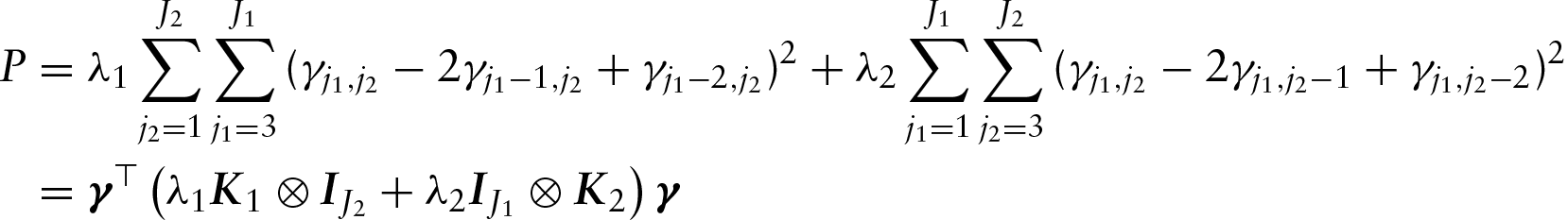
\begin{array}{l} P = λ_{1} \sum_{J_{2} = 1}^{J_{2}} \sum_{j_{1} = 3}^{J_{1}} {(γ_{j 1, j 2} - 2 γ_{j 1 - 1, j 2} + γ_{j 1 - 2, j 2})}^{2} + λ_{2} \sum_{J_{1} = 1}^{J_{1}} \sum_{j_{2} = 3}^{J_{2}} {(γ_{j 1, j 2} - 2 γ_{j 1, j 2 - 1} + γ_{j 1, j 2 - 2})}^{2} \\ = γ^{T} (λ_{1} K_{1} \otimes I_{J 2} + λ_{2} I_{J 1} \otimes K_{2}) γ \end{array}

to penalize the surfaces wiggliness. Therefore, $K_{k}$ are the penalty matrices in each direction $k = 1, 2$ and $I_{J_{k}}$ are identity matrices with dimension corresponding to the number of basis function in the other direction. More details on this idea can also be found in Fahrmeir et al. (2013).

2.3 Spatio-temporal models

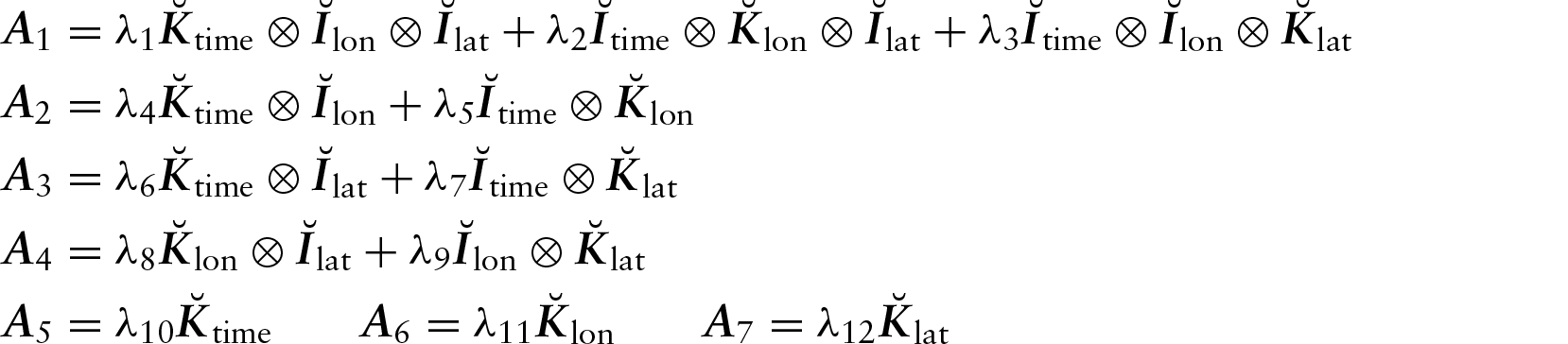
In analogy to the interaction between two covariates, we can use the aforementioned strategy to build interactions in any dimensions (see Wood, 2006). An application of a trivariate interaction is the temporal variation of a spatial effect (or, vice versa, the spatial variation of a temporal effect) in a spatio-temporal model. Therefore, we build the trivariate smooth surface based on the univariate basis functions as

f ({time}_{i}, {lon}_{i}, {lat}_{i}) = (B_{i, time} \otimes B_{i, lon} \otimes B_{i, lat})^{⊤} γ,

(2.1)

where lon and lat represent the longitudinal and the latitudinal coordinate of an observation, respectively. Furthermore, γ is now a new vector of coefficients corresponding to the design matrix. Moreover, the penalty term is then defined as

\begin{matrix} P & = γ^{⊤} (λ_{time} K_{time} \otimes I_{J_{lon}} \otimes I_{J_{lat}} + λ_{lon} I_{J_{time}} \otimes K_{lon} \otimes I_{J_{lat}} + λ_{lat} I_{J_{time}} \otimes I_{J_{lon}} \otimes K_{lat}) γ \end{matrix}

with penalty matrices $K_{k}$ as introduced earlier in this article.

The identifiability of semiparametric regression has, in this article, not been discussed so far. Applying several basic univariate P-splines in one model is not identified since each smooth function could be shifted on the y-axis and the shift would be absorbed by the intercept or another smooth function. Therefore, the identifiability constraint $\sum_{i} f_{k} (x_{ik}) = 0$ is included. One approach to achieve this constraint is based on the eigen decomposition of the penalty matrix. As a result, for each univariate P-spline the intercept of each spline corresponds to one eigenvalue equal to zero, which could be excluded (for more details see Fahrmeir et al. [2004] for example). Based on the resulting diagonal penalty matrix, the approach is called mixed models decomposition. Applying the decomposition on multidimensional P-splines has the effect that the marginal splines can be separated from the interaction term. So we can separate the main effects from the interaction term. This so-called ANOVA decomposition was discussed in Gu (2002), Lee and Durbán (2011), Lee et al. (2013), Wood et al. (2013) and Kneib et al. (2017).

An alternative approach to achieve identifiability is to transform the basis functions and the penalty matrices with a QR-decomposition of the vector of column means of $B_{k}$ (see Wood [2017] Section 5.4.1 and Section 1.8.1 for details). In a higher dimensional setting, this procedure could be adopted, such that first the multidimensional basis functions (based on the unconstrained marginal basis functions) and penalties are built and afterward the QR-decomposition is applied to guarantee identifiability. This would result in the standard multidimensional interaction surface without separate main effects. To determine the separate main effects, the order of the QR-decomposition and the Kronecker product is interchanged. Thus, the multi-dimensional basis function is build as Kronecker product of the univariate basis functions which have already been transformed based on the QR-decomposition. To get valid estimates, the marginal basis functions must be added to the design matrix. Therefore, the design matrix of the spatio-temporal model with separate main effects has the following structure

[1 : {\overset{⌣}{B}}_{time} □ {\overset{⌣}{B}}_{lon} □ {\overset{⌣}{B}}_{lat} : □ {\overset{⌣}{B}}_{time} □ {\overset{⌣}{B}}_{lon} : □ {\overset{⌣}{B}}_{time} □ {\overset{⌣}{B}}_{lat} : □ {\overset{⌣}{B}}_{lon} □ {\overset{⌣}{B}}_{lat} : □ {\overset{⌣}{B}}_{time} : □ {\overset{⌣}{B}}_{lon} : □ {\overset{⌣}{B}}_{lat}]

(2.2)

where ${\overset{⌣}{B}}_{k}$ are the marginal basis functions including the transformation based on the QR-decomposition. Here, $□$ is the row-wise Kronecker product, for matrices as used in Lee and Durbán (2011) and defined in Eilers et al. (2006). Based on this definition, ${\overset{⌣}{B}}_{time} γ_{time}$ build the main effect for time and ${\overset{⌣}{B}}_{lon} □ {\overset{⌣}{B}}_{lat} γ_{lon \times lat} + {\overset{⌣}{B}}_{lon} γ_{lon} + {\overset{⌣}{B}}_{lat} γ_{lat}$ the main effect for space with corresponding subvectors of γ. Thus, we separate the main effects from the interaction effects. Since the transformed basis functions ${\overset{⌣}{B}}_{k}$ have one column less than $B_{k}$ , the dimensions of Equation (2.1) and Equation (2.2) coincide. Similarly, the penalty matrix is now build as a block diagonal matrix $K_{λ} = diag (0, A_{1}, A_{2}, A_{3}, A_{4}, A_{5}, A_{6}, A_{7})$ with values

\begin{matrix} A_{1} & = λ_{1} {\overset{⌣}{K}}_{time} \otimes {\overset{⌣}{I}}_{lon} \otimes {\overset{⌣}{I}}_{lat} + λ_{2} {\overset{⌣}{I}}_{time} \otimes {\overset{⌣}{K}}_{lon} \otimes {\overset{⌣}{I}}_{lat} + λ_{3} {\overset{⌣}{I}}_{time} \otimes {\overset{⌣}{I}}_{lon} \otimes {\overset{⌣}{K}}_{lat} \\ A_{2} & = λ_{4} {\overset{⌣}{K}}_{time} \otimes {\overset{⌣}{I}}_{lon} + λ_{5} {\overset{⌣}{I}}_{time} \otimes {\overset{⌣}{K}}_{lon} \\ A_{3} & = λ_{6} {\overset{⌣}{K}}_{time} \otimes {\overset{⌣}{I}}_{lat} + λ_{7} {\overset{⌣}{I}}_{time} \otimes {\overset{⌣}{K}}_{lat} \\ A_{4} & = λ_{8} {\overset{⌣}{K}}_{lon} \otimes {\overset{⌣}{I}}_{lat} + λ_{9} {\overset{⌣}{I}}_{lon} \otimes {\overset{⌣}{K}}_{lat} \\ A_{5} & = λ_{10} {\overset{⌣}{K}}_{time} A_{6} = λ_{11} {\overset{⌣}{K}}_{lon} A_{7} = λ_{12} {\overset{⌣}{K}}_{lat} \end{matrix}

where ${\overset{⌣}{K}}_{k}$ are the penalty matrices of the marginal basis functions including the transformation based on the QR-decomposition. Therefore, ${\overset{⌣}{I}}_{k}$ are of one dimension less than $I_{k}$ . Based on this decomposition, we can determine the main effects separately from their interactions (Wood (2017) p. 232). Thus, we interpret the marginal spatial and the temporal effect separately from the interaction.

The separation as mixed models and the separation based on the QR decomposition results in the same predictions if appropriate smoothing parameters are chosen. However, we focus here on the separation based on the QR decomposi- tion since this is included in the mgcv package, which allows for using large datasets. More details are discussed in Section 3.2.

2.4 Regional data

So far, we estimated the spatial trend based on the exact longitudinal and latitudinal coordinates of the location. In many datasets, however, the location is only measured in regional grids such as ZIP-code areas or states. A simple model would use the regional information as a factor variable and estimate independent effects for each region. However, this results in rather wiggly estimates comparing neighbouring regions. Therefore, our goal is to estimate a smooth surface of the spatial effect also with regional data. Generally, the smoothed regional effects approach is motivated by Gaussian Markov random fields (GMRF; Rue and Held, 2005). The spatial surfaces based on the categorical covariates can be estimated as smooth effects $f (s_{i}) = B_{i, GMRF}^{⊤} ν$ , where $s_{i}$ is the region in which $y_{i}$ was observed. The coefficients $ν = (ν_{1}, \dots, ν_{S})$ define the effect for each of the $S$ regions.

For estimation, the design matrix of the regional covariate $B_{GMRF}$ is build as an indicator matrix, that is, the $i$ th row of $B_{GMRF}$ is defined as the vector with elements

\begin{matrix} B_{i, GMRF} = \{\begin{matrix} 1 & if y_{i} was observed in region s, \\ 0 & otherwise . \end{matrix} \end{matrix}

To get a smooth effect, differences between neighbouring regions are penalized with a penalty matrix $K_{GMRF}$ whose elements are defined as

\begin{matrix} K_{{GMRF}_{sr}} = \{\begin{matrix} - 1 & , if s \neq r and s \sim r \\ 0 & , if s \neq r and s ≁ r \\ total number of neighbours of s & , if s = r \end{matrix} \end{matrix}

where $s \sim r$ denotes that $s$ is a neighbour of $r$ . The coefficients $ν$ are then estimated with penalized likelihood methods similarly to P-splines. Due to the similarities of GMRF and P-splines as penalized models, they can also interact in a spatio-temporal model. Therefore, we define the design matrix similarly as in Equation (2.2) as matrix

\begin{matrix} [1 : {\overset{⌣}{B}}_{time} □ {\overset{⌣}{B}}_{GMRF} : {\overset{⌣}{B}}_{time} : {\overset{⌣}{B}}_{GMRF}] \end{matrix}

with ${\overset{⌣}{B}}_{GMRF}$ being the centred indicator matrix $B_{GMRF}$ . Furthermore, the spatio-temporal penalty matrix is defined as the block diagonal matrix

\begin{matrix} K_{λ} = diag (0, λ_{1} {\overset{⌣}{K}}_{time} \otimes {\overset{⌣}{I}}_{GMRF} + λ_{2} {\overset{⌣}{I}}_{time} \otimes {\overset{⌣}{K}}_{GMRF}, λ_{3} {\overset{⌣}{K}}_{time}, λ_{4} {\overset{⌣}{K}}_{GMRF}), \end{matrix}

where ${\overset{⌣}{K}}_{GMRF}$ is the penalty matrix for the spatial effect considering the centring. ${\overset{⌣}{K}}_{time}$ and $\overset{⌣}{I}$ are defined as mentioned earlier in this article.

3 Expectile regression

The classical linear model is based on the assumption of homoscedasticity. If this assumption is violated, the standard estimators for the mean effects are still valid while the estimation of their uncertainty is not valid anymore. Moreover, we are then interested what the drivers for the heteroscedasticity are and how they influence the response. There are several models, that allow for heteroscedastic error terms and analyse the drivers, including GAMLSS (Rigby and Stasinopoulos, 2005) and quantile regression (Koenker and Bassett, 1978). As discussed in the introduction, we will apply expectile regression as introduced by Newey and Powell (1987) in this article. For the introduction of expectile regression, we start with only linear effects in Section 3.1, before we introduce semiparametric expectile regression in Section 3.2.

3.1 Classical expectile regression

In ordinary least squares models, the sum of squared residuals should be minimized with respect to the regression coefficients. Taking the derivative of the least squares equation with respect to these coefficients and setting it to zero yields the least squares estimate. Furthermore, rearranging the derivative with respect to the intercept shows that the sum of the residuals must be 0. Thus, the solution will be the predictor, where the sum of the residuals above and below are equal which corresponds to the centre, of gravity in a physical interpretation. In expectile regression, the emphasis is now put on outer parts of the distribution to detect variation of the effects beyond the mean. Therefore, in the least squares equation, a weight $w_{τ} (y_{i})$ is included such that observations $y_{i}$ below the fitted effect $x_{i}^{⊤} {\hat{β}}_{τ}$ get another weight than the observations above, yielding

\hat{β} =_{β_{τ}}^{argmin} \sum_{i = 1}^{n} w_{τ} (y_{i}) {(y_{i} - x_{i}^{T} β_{τ})}^{2},

(3.1)

where the weights are defined as

\begin{matrix} w_{τ} (y_{i}) & = \{\begin{matrix} τ & if & y_{i} \geq x_{i}^{⊤} {\hat{β}}_{τ} \\ 1 - τ & if & y_{i} < x_{i}^{⊤} {\hat{β}}_{τ} \end{matrix} . \end{matrix}

Thereby the predictor $x_{i}^{⊤} {\hat{β}}_{τ}$ depends on the specified asymmetry parameter $τ \in (0, 1)$ . Based on this definition, the 50% expectile coincides with the ordinary mean while fitted expectiles provide a weighted centre of gravity. As discussed before, in classical linear regression, the error terms $ε_{i} = y_{i} - x_{i}^{⊤} β$ are assumed to be independent and identically normally distributed ( $ε_{i} \sim N (0, σ^{2})$ ). Contrarily, in expectile regression we do not assume any parametric distribution for the error terms $ε_{i, τ} = y_{i} - x_{i}^{⊤} β_{τ}$ , nor do we assume identically distributed error terms. The only constraint besides independent error terms is that the expectile of interest is 0 for the error terms (this is in complete analogy to assuming that the quantile of the error terms is equal to 0 in quantile regression; see Schnabel and Eilers [2009] and Schulze Waltrup et al. [2015] for details).

\begin{matrix} E (w_{τ} (ε_{i, τ}) {(ε_{i, τ} - {\hat{e}}_{i, τ})}^{2}) = 0 . \end{matrix}

The solution for Equation (3.1) can be written in matrix notation as

\begin{matrix} {\hat{β}}_{τ} = {(X^{⊤} W_{τ} X)}^{- 1} X^{⊤} W_{τ} y, \end{matrix}

where $W_{τ}$ is the diagonal matrix of weights $w_{τ} (y_{i})$ . As a consequence, standard weighted least squares techniques can be applied for the estimation of ${\hat{β}}_{τ}$ . The only problem is that $W_{τ}$ depends on ${\hat{β}}_{τ}$ and vice versa. So the optimization of ${\hat{β}}_{τ}$ and $w_{τ} (y_{i})$ is done iteratively with an algorithm called least asymmetric weighted squares (Schnabel and Eilers, 2009), where we start with a classical linear model with equal weights for all observations. Afterwards, the new weights are estimated and a new weighted model is fitted. The estimation of weights and coefficients is iterated until the weights remain unchanged. The estimated coefficients ${\hat{β}}_{τ}$ asymptotically follow a normal distribution (Sobotka et al., 2013). However, in the setting of spatio-temporal models, the number of observations is usually huge (in our example we have more than $4.3 \cdot 10^{6}$ observations) therefore the confidence intervals will be very small. Thus, we omit them in the following.

3.2 Smoothing parameter determination in spatio-temporal expectile regression

In Section 3.1, we defined expectile regression for linear predictors. In order to gain more flexibility, semiparametric predictors are useful. Therefore, Schnabel and Eilers (2009) and Sobotka and Kneib (2012) introduced semiparametric expectile regression with the penalized LAWS criterion

\sum_{i = 1}^{n} w_{τ} (y_{i}) {(y_{i} - x_{i}^{T} γ_{τ})}^{2} + γ_{τ}^{T} K_{λ} γ_{τ} .

(3.2)

To simplify notation, $x_{i}$ is now not the pure vector of covariates, but the joint vector of covariates for linear effects and evaluated basis functions for smooth effects. Furthermore, $γ_{τ}$ is the vector of all coefficients corresponding to linear and smooth effects. Thus, $x_{i}^{⊤} γ_{τ}$ is the semiparametric predictor of linear effects and smooth functions dependent on the smoothing parameters and the asymmetry τ. $K_{λ}$ is the penalty matrix including the smoothing parameters, which are dependent on the asymmetry. Due to the technical equivalence between weighted linear regression and expectile regression, this is straightforward. So spatio-temporal models can also be applied in expectile regression. In the estimation, the critical point is the optimization of the smoothing parameters λ. It has to be done from outside the LAWS algorithm since otherwise the iteration does not always converge. Generally, there exist two ideas for the optimization: Either using goodness-of-fit criteria or applying ideas of mixed model-based estimation.

In our application, we use the power (both with respect to memory requirement and computational speed) of the mgcv package of Wood (2017) in the statistical programming environment R (R Core Team, 2017) to estimate spatio-temporal expectile models via weighted least squares. The bam function of the mgcv package was optimized to reduce the memory demand by avoiding to calculate the design matrix and applying other smart tricks (see ; Wood et al. [2015; 2017] for details). The exact code for estimating expectile regression with spatio-temporal effects is attached in the supplementary material. Basically, in the inner loop we fix the smoothing parameters and estimate the LAWS algorithm, with help of the function bam. Then we apply standard numerical optimization routines to optimize the smoothing parameters from outside. The asymmetric GCV criterion

\frac{n \sum_{i = 1}^{n} w_{τ} (y_{i}) {(y_{i} - x_{i}^{T} {\hat{γ}}_{τ})}^{2} + γ_{τ}^{T} K_{λ} γ_{τ} .}{{((trace (I - H))}^{2}}

proved to have good properties in Schnabel and Eilers (2009) as a criterion for the optimization. Moreover, it is straightforward to the classical optimization of smoothing parameters in the model based on homoscedastic Gaussian distributed errors (see Wood, 2017). In the earlier formula, I is an identity matrix of dimension $n \times n$ and $H = W_{τ}^{1 / 2} X (X^{⊤} W_{τ} X + K_{λ})^{- 1} X^{⊤} W_{τ}^{1 / 2}$ is the hat matrix. More details on the estimation of semiparametric expectile regression in general are presented in Sobotka and Kneib (2012).

Due to the possibility to write P-splines as mixed models, the Schall algorithm (Schall, 1991) for selecting smoothing parameters was introduced to semiparametric expectile regression by Schnabel and Eilers (2009). However, the Schall algorithm only allows for one smoothing parameter per smooth term, since it needs a standard form in the penalty matrix (see Wood and Fasiolo 2017, p. 3 or Rodríguez-Álvarez et al.2015, p. 943). Thus, the Schall algorithm is not applicable in spatio-temporal models, where we have multiple smoothing parameters per smooth term. Alternatively, the generalized Fellner–Schall algorithm of Wood and Fasiolo (2017) can be adopted to semiparametric expectile regression by interpreting expectile regression as weighted linear regression. Moreover, the generalized Fellner–Schall algorithm allows for the estimation of smoothing parameters in interaction settings. Other approaches such as Lee et al.(2013), Rodríguez-Álvarez et al. (2015) and Rodríguez-Álvarez et al. (2018) also provide powerful extensions to the standard approach of Schall (1991) for interaction settings. These approaches could also be used in expectile regression due to the equivalence to weighted least squares. However, the Fellner–Schall algorithm for expectile regression can be implemented based on the memory saving algorithms of the mgcv package, while the other approaches all need the calculation of the design matrix, which is expensive if not prohibitive. In our example in the 50% expectile case, we only needed approximately 5GB RAM using the Fellner–Schall approach, while we had to stop the SAP algorithm of the supplementary material of Rodríguez-Álvarez et al.(2015) at 180GB to prevent our server from crashing. Moreover, the available SAP algorithm does not account for additional covariates. So we only provide here the Fellner–Schall algorithm additionally to the GCV optimization.

In the generalized Fellner–Schall algorithm, the smoothing parameters are optimized iteratively with the model fit. So the model is estimated given some smoothing parameters λ. Thus, $W_{τ}$ and ${\hat{γ}}_{τ}$ are the respective weights and the estimated coefficients of the expectile regression given the old smoothing parameters λ. Afterwards preliminary smoothing parameters are fitted as

\begin{matrix} λ_{k}^{*} = ϕ \frac{tr (K_{λ}^{-} S_{k}) - tr ((X^{⊤} W_{τ} X + K_{λ})^{- 1} S_{k})}{{\hat{γ}}_{τ}^{⊤} S_{k} {\hat{γ}}_{τ}} λ_{k}, \end{matrix}

(3.3)

where $ϕ$ is a scaling parameter based on the variance and $K_{λ}^{-}$ is the Moore–Penrose pseudoinverse of the full penalty matrix $K_{λ}$ including the old smoothing parameters λ. Furthermore, $S_{k}$ is similar to $K_{k}$ (or ${\overset{⌣}{K}}_{k}$ ), the penalty matrix corresponding to one effect $k$ . However, $S_{k}$ is of the same dimensions as the complete penalty matrix $K_{λ}$ , so it is padded with zeros at all elements that do not correspond to the effect $k$ . Nevertheless, $S_{k}$ does not include the factor $λ_{k}$ . In detail, we specify the block diagonal matrix $S_{k} = (0, \dots, 0, K_{k}, 0, \dots, 0)$ . In the estimation of new smoothing parameters, some kind of step halving is established to ensure a better model fit in each iteration. Therefore, we define λ as the old smoothing parameters, $λ^{*}$ as the vector of preliminary smoothing parameters calculated via Equation (3.3) and $λ^{new}$ as the final new smoothing parameter of this iteration. Via step halving, the new smoothing parameters are calculated as

\begin{matrix} λ^{new} = \frac{λ^{*} - λ}{2^{p}} + λ, \end{matrix}

where $p = 0, 1, 2, \dots$ is the minimal integer such that the goodness of fit decreases. Therefore, either the penalized LAWS criterion as defined in Equation (3.2) or the GCV can be applied. The generalized Fellner–Schall algorithm has some numerical drawbacks. First, calculating $(X^{⊤} W_{τ} X + K_{λ})^{- 1}$ is computationally burdensome, but it is estimated anyway for the standard confidence intervals (see, e.g., Marra and Wood, 2012). Thus, these estimates can be reused. Second, estimating $K_{λ}^{-}$ is only possible if the smoothing parameters are in an appropriate range, otherwise the pseudoinverse will vanish. Therefore, we have to restrict the possible smoothing parameters and fix them, if they reach the limit. This drawback could be avoided when using the SOP algorithm of Rodríguez-Álvarez et al. (2018), however then the drawbacks with the memory usage would occur again.

Alternatively to expectile regression, quantile regression (Koenker and Bassett, 1978; Koenker, 2005) can be used to estimate models beyond the mean. Therefore, in Equation (3.1), the $l_{2}$ -norm is exchanged with the $l_{1}$ -norm. In quantile regression, the fitted effects represent the line where the ratio of numbers of observations below and above is the desired fraction τ, while in expectile regression the fitted values give the weighted centre of gravity, so the line where the sum of the weighted distances below and above coincides with the given fraction τ (Yao and Tong, 1996). So quantile regression only checks how many observations are below and above the fitted values. The distance between the fitted values and the observations is not taken into account. Since expectiles account also for the values of the distances, it uses more information while, on the downside, becoming more susceptible for the influence of outliers. Moreover, applying quantile regression instead of expectile regression in the spatio-temporal setting would hardly be possible due to the smooth trivariate interactions of space and time. Quantile regression relies on the $l_{1}$ -norm and therefore no derivatives can be used to optimize the model. The linear programming routines solving quantile regression are computationally more challenging in combination with penalized estimation than the LAWS algorithm. In our approach of using trivariate smooth interactions to model the spatial and temporal interaction, we need more than 800 coefficients and 14 smoothing parameters. Optimizing such a model with linear programming routines is time consuming. However, there are approaches that tackle the spatial and spatial temporal dependence of effects in quantile regression. Reich et al. (2011) and Reich (2012), for example, estimate different time coefficients at each location and smooth them in a second step. This is done in a Bayesian setting. However, they need to apply some approximations to get the spatial dependence and to be able to deal with a larger number of observations. Contrarily to our smooth time effect, they rely on a linear time trend.

4 Simulation study

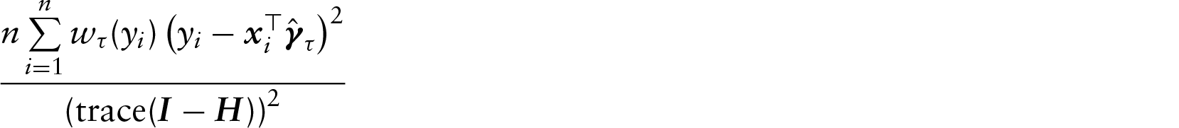
Applying the GCV to select smoothing parameters in semiparametric expectile regression with interactions is straightforward. Nevertheless the generalized Fellner–Schall algorithm has, to our knowledge, never been used in expectile regression before. Therefore, we provide in this section a small simulation study to compare the goodness of fit of both approaches.

The covariates $x_{1}, x_{2}$ are simulated based on the standard uniform distribution ( $x_{1}, x_{2} \sim U (0, 1)$ ). As distribution of the error terms, a Gaussian distribution is assumed $(ε_{i} \sim N (0, σ_{i}^{2}))$ . However, for the variance either homoscedasticity ( $σ_{i} = 2 \forall i$ ) or heteroscedasticity ( $σ_{i} = \frac{x_{i 1} + 1}{1.5} + \frac{x_{i 2} + 1}{1.5}$ ) is considered. As covariate effects, we use two different functions, similarly as in Wood (2006):

\begin{matrix} f_{1} (x_{1}, x_{2}) & = 1.2 π (1.2 e^{- (x_{1} - 0.2)^{2} / 0 . 3^{2} - (x_{2} - 0.3)^{2} / 0 . 4^{2}} + 0.8 e^{- (x_{1} - 0.7)^{2} / 0 . 3^{2} - (x_{2} - 0.8)^{2} / 0 . 4^{2}}) \\ f_{2} (x_{1}, x_{2}) & = 2 \sin (π x_{1}) + \exp (2 x_{2}) . \end{matrix}

Here $f_{1}$ represents an interaction setting of the covariates, while $f_{2}$ represents an additive setting of the covariates. Finally, the response is defined as $y_{i} = f_{j} (x_{i 1}, x_{i 2}) + ε_{i}$ . For each replication, a dataset with 5 000 observations is simulated to fit the model and for all replications an independent test dataset with 10 000 observations is used to estimate the predictive mean weighted squared error (PMWSE) as measure for the goodness of fit, that is,

PMWSE = \sum_{i = 1}^{n} w_{τ} (y_{i}) {(y_{i} - x_{i}^{T} {\hat{γ}}_{τ})}^{2} .

Overall, 100 independent replications of expectile models with $τ \in (0.01, 0.02, 0.5, 0.1, 0.5, 0.9, 0.95, 0.98, 0.99)$ are applied. For the estimation, the model is specified with separation of main effects as

\begin{matrix} y \sim f (x_{i 1}) + f (x_{i 2}) + f (x_{i 1}, x_{i 2}) \end{matrix}

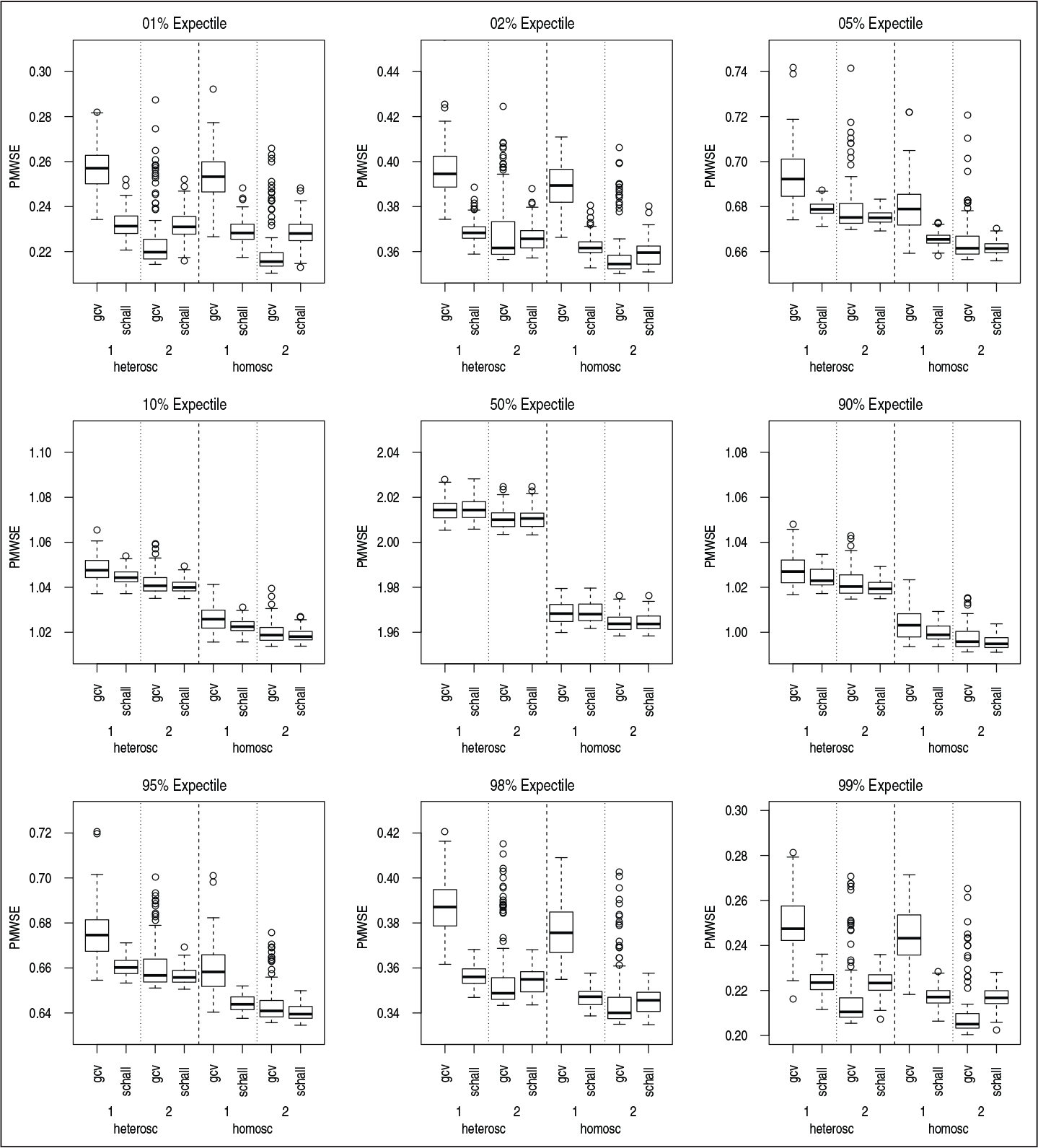
with 15 B-spline basis functions in each direction. Since the smoothing parameters in the Fellner–Schall algorithm have to be sized neither too small nor too large, we restrict them to be larger than $10^{- 5}$ and smaller than $10^{5}$ . For improved comparability, this restriction is also applied in the GCV approach. Figure 1 shows the PMWSE of the estimated models. In each plots the range has a size of 0.10, but the y-axis is shifted. Without any constraint on the range of the y-axis the plots would be less comparable, while the same limits for all plots would result in too small graphics to be interpretable. Thus, we decided to fix the range to 0.1, but let the absolute values of the limits vary between the figures.

For the central asymmetries, similar outputs for the optimization via GCV and generalized Fellner–Schall occur. Comparing more extreme asymmetries results in differences between the optimization methods. The Fellner–Schall algorithm has benefits in the interaction setting ( $f_{1}$ ), while the GCV has advantages in the additive setting ( $f_{2}$ ). However, no clear overall advantage of one method is detectable. Additionally, the simulation study was also applied with fewer observations ( $n = 2 000$ ). There the same pattern are detected. Thus, we show the results in the supplementary material only. Further analyses shows that the generalized Fellner–Schall algorithm is more dependent on the starting values.

Figure 1:

PMWSE of the simulation study

5 Spatio-temporal analysis of temperatures in Germany

The distribution of temperatures in Germany motivated us for a spatio-temporal estimation beyond the mean. Therefore, we use data from the German weather service (DWD, 2017). The response variable is the daily mean temperature in $^{\circ} C$ . Since we are interested in analysing the variation within years, the aggregation on the average per day does not impair the expectile regression. In this example, we use all stations with at least 24 years of observations in the period 1980 to 2014. Furthermore, stations above 900m are included if they have at least 3 650 values, but the station on top of the ‘Zugspitze’ is excluded, due to fitting problems based on the large gap in the elevation scale. So finally we use data of 374 stations, whose locations are visualized in Figure 2. 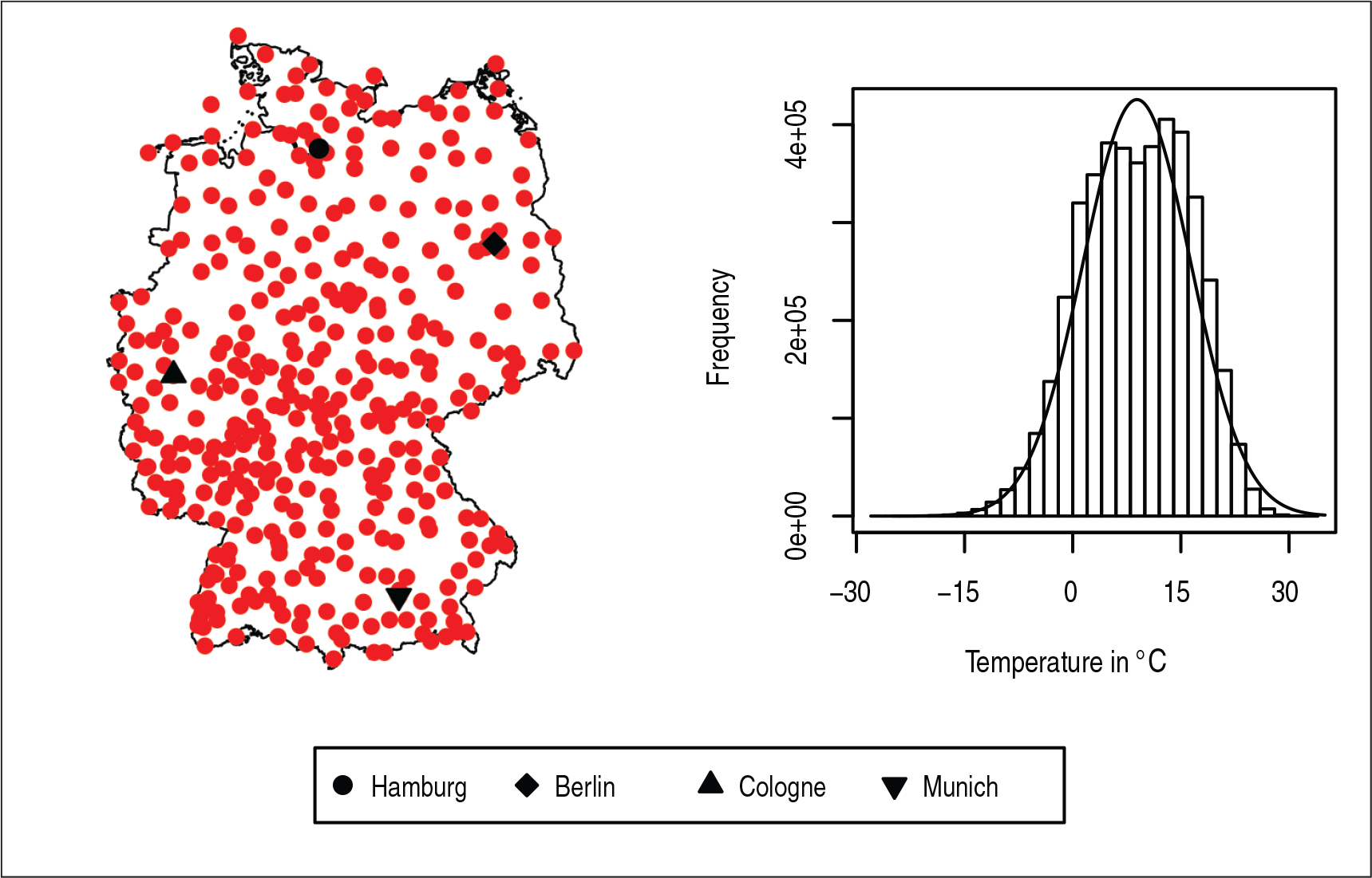On the right side of this figure, the marginal frequencies of the daily mean temperature from 1980 to 2014 are plotted jointly with a Gaussian density of appropriate mean and standard deviation. Even if the marginal density fits well with the Gaussian density, we model the spatio-temporal distribution of the daily temperatures with spatio-temporal expectile regression in the following. Doing so, we get not only information on the general temperature pattern in Germany in different seasons of the year but also information on areas where at distinct time points the spectrum of temperatures is wider or smaller.

Figure 2:

Location of the observation stations and marginal density of daily mean temperature

To model the spatial and temporal variation of the temperatures (in $^{\circ} C$ ), we apply the following model

\begin{matrix} temperature & = β_{0, τ} + f_{τ} (elevation) + f_{τ} (year) + f_{τ} (day) + f_{τ} (lon) + f_{τ} (lat) \\ + f_{τ} (day, lon) + f_{τ} (day, lat) + f_{τ} (lon, lat) + f_{τ} (day, lon, lat) + ε_{τ} \end{matrix}

for each asymmetry parameter $τ \in$ (0.01, 0.02, 0.5, 0.1, 0.2, 0.5, 0.8, 0.9, 0.95, 0.98, 0.99) separately. In the models, elevation is the altitude above sea level of the observation station (in meters), while longitude (lon) and latitude (lat) specify the location in Greenwich coordinates. With day, the day of the year is meant. Here we consider the spatio-temporal effect to be identical for multiple years. To get a smooth transition for December to January, we apply cyclic P-splines for the temporal effect as discussed in de Boor (1978) and Wood (2017). The variation between the years is considered via an additive smooth effect. Alternatively, an interaction between the year of the observation and the spatio-temporal model could be interesting to analyse the climate change. However, with this four-dimensional covariate structure we would run into trouble with the curse of dimensionality (Fahrmeir et al., (2013), p. 531). The same argument applies for an interaction between the spatio-temporal part and the elevation.

As discussed in Section 2.3, the effects $f_{τ} (day)$ , $f_{τ} (lon)$ , $f_{τ} (lat)$ , $f_{τ} (day, lon)$ , $f_{τ} (day, lat)$ , $f_{τ} (lon, lat)$ , $f_{τ} (day, lon, lat)$ represent the ANOVA-type decomposition of the spatio-temporal model, similarly as introduced in Wood (2006), Lee and Durbán (2011) and Lee et al.(2013) for example. Therefore, each of these effects corresponds to its own smoothing parameters. However, we are here mainly interested in the time effect $f_{τ} (day)$ , the spatial effect $f_{τ} (day, lon)$ and the interaction between time and space $f_{τ} (day, lon, lat)$ . Thus, the univariate spatial effect in longitudinal or latitudinal direction only ( $f_{τ} (lon)$ , $f_{τ} (lat)$ ) as well as the interaction of the one-dimensional spatial effects with time ( $f_{τ} (day, lon)$ , $f_{τ} (day, lat)$ ) are just included to get a valid design matrix and are interpreted jointly with $f_{τ} (lon, lat)$ and $f_{τ} (day, lon, lat)$ .

For the estimation, we apply penalized cubic B-splines with 15 basis functions for the spline of the year. Moreover, the spatio-temporal effect has 15 basis functions for the daily effect and 6 respectively 9 basis functions for the univariate spatial marginals. The spatial effect has only few basis functions in each direction to obtain reasonable computational times. Furthermore, with a higher number of basis functions, we obtain instabilities at the borders due to the small number of observation stations in certain regions close to the German border. Lee et al. (2013) proposes to use different number of basis function in nested designs. However, then we would assume that in the main effects more information is contained than in the interaction, which we do not assume in our model. For the estimation of the elevation effect, only 7 basis functions are applied to avoid arbitrary results due to gaps in the parameter space. The smoothing parameters are optimized via GCV (see Section 3.2). The results for optimizing the smoothing parameters via the generalized Fellner–Schall algorithm are similar and available on demand.

In Figure 3, the estimated main effects for elevation and day are displayed. We see some variation between the mean effects and the effects at the outer parts of the distribution. While for the low areas the curves are parallel, which indicates homo- scedasticity, the outer expectile curves diverge from the mean for higher altitudes. The difference looks rather small, but we are talking about $2^{\circ} C$ difference between the 10% and the 90% expectiles. Thus, heteroscedasticity occurs in these areas.

Figure 3:

Main effects for elevation, day and year (including intercept)

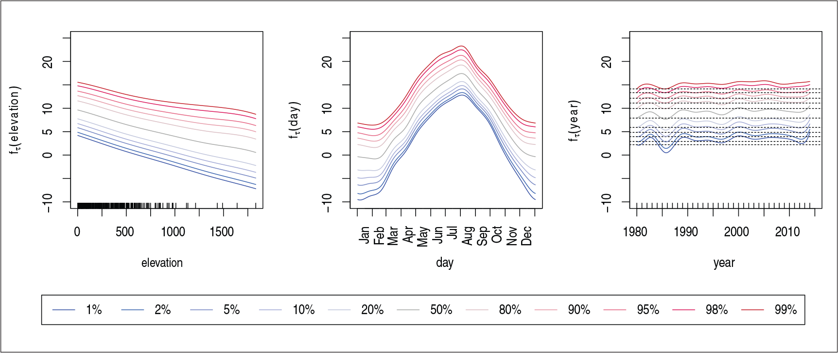
For the main effect of the day in the year, as displayed in Figure 3 in the middle picture, we can detect that the lower expectiles have a wider range than the upper expectiles. This means, in winter the lower temperatures are often lower than expected and in summer the low temperatures are higher than expected. Moreover, the difference between the lower expectile and the upper expectile is in winter higher than in the summer. Thus, the expected variance of temperatures in winter is higher than in summer. Furthermore, the high temperatures in summer are not as high as they had to be if the underlying process was a homoscedastic Gaussian distribution.

By including the parameter year in the model, we control for varying effects in specific years. Additionally, we can check if we find some impact of the climate change in this rather small example. The estimated curve for the trend per year is also plotted in Figure 3 on the right. There we detect some small general increase in the temperatures, beyond the natural fluctuation.

The spatio-temporal result for $τ \in (0.1, 0.5, 0.9)$ is displayed in Figure 4 in terms of the spatial effect for 31 January and 31 July. The trends are also valid for the other asymmetry levels, which are displayed in the supplementary material. The colours of both rows follow the same legend, the steps between the contour lines /colour codes are $1^{\circ} C$ . From Figure 4 we can conclude two things. The most obvious one is that the spatial effect in January is different from July, since in January it gets colder from west to east, while in summer the north is colder than the south. On the other hand, the variation from the mean is visible. So is the coast of the Baltic Sea a lot warmer in cold winters than expected for this location. Furthermore, the coldest winters are detected east of Berlin, while there is a rather constant effect for this area at the $90 %$ expectile for 31 January. In general the variation of temperatures on 31 January is larger for the lower expectile than for the upper expectile. Moreover, in northern Germany the variation for cold summers ( $10 %$ expectile) is rather low, while there is a clear cooling towards the sea for warm summers. Similar patterns can be found for the prediction including the elevation.

Figure 4:

Prediction of the spatial effect for 31 January and 31 July, excluding elevation and intercept

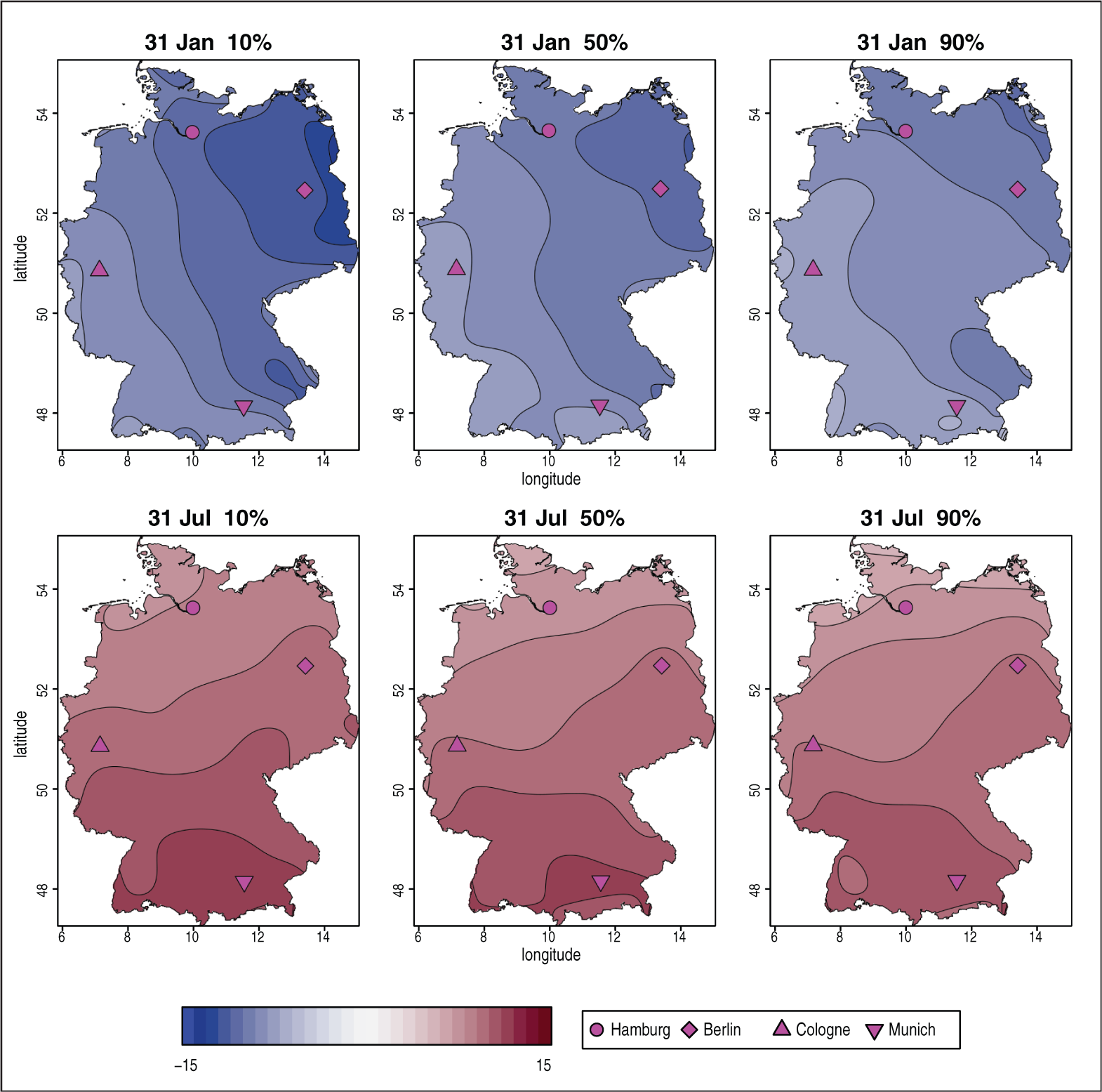
To get a better impression on how the spatial effect varies with time, we plotted the temporal effect of four German cities in the supplementary material. Their locations are indicated in the spatial effect maps. Out of this figure, we conclude that in Cologne the winters are a lot warmer than in Munich or Berlin, while the summers are colder in Hamburg and warmer in Berlin. This differentiation is valid for all parts of the distribution, but the amplitude of the temperatures is smaller for the upper part of the distribution than for the lower part.

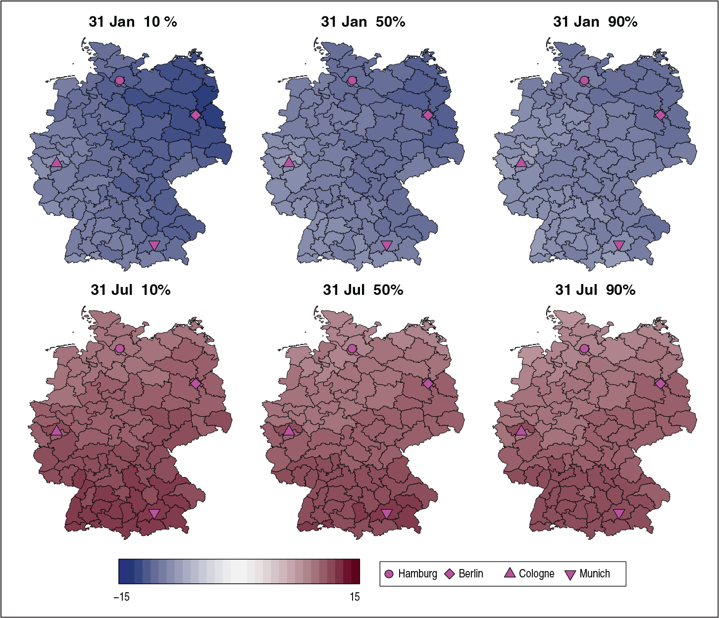
Additional to the application of the exact location of the observation stations, we apply the same data but with locations on a regional level. Therefore, we assign to each location its ‘Raumordnungsregion’ (BBSR, 2017). The ‘Raumordnungsregion’ is a special German classification of regions between the NUTS 2 and NUTS 3 level. The advantage of this grid is that the 96 regions have similar size and we have for each region at least one observation station (with region 506, Dortmund, as the single exception without an observation station which is therefore merged with region 509, Emscher-Lippe). To model the spatio-temporal trend based on grid data, we then use the model of Section 2.4, while the rest of the covariate information remained unchanged. Thus, the model is built as

\begin{matrix} temperature & = β_{0, τ} + f_{τ} (elevation) + f_{τ} (year) + f_{τ} (day) + f_{τ} (region) \\ + f_{τ} (day, region) + ε_{τ} . \end{matrix}

As expected, the effects for year and elevation as well as the seasonal trend are similar in this grid approach, compared to the original model. Also the spatial patterns as displayed in Figure 5 show a large similarity to the spatial effect based on the exact locations of Figure 4. We still observe an east–west trend in winter and a north–south trend in summer. Furthermore, the variation for colder winter is higher than for warmer winters.

Figure 5:

Prediction of the regional effect for 31 January and 31 July, excluding elevation and intercept

All code and data to reproduce the analysis of this article are included in the online supplementary material.

6 Conclusion

In this article, we present spatio-temporal effects for expectile regression. Spatio-temporal modelling with interaction terms of P-splines is nowadays a well established method. However, usually the data are analysed with some pre-specified parametric distribution and the errors are assumed to be homoscedastic. Contrarily, in expectile regression no assumption on the distribution of the data is applied. Moreover, expectile regression is able to take heteroscedasticity of the data into account. Based on the idea of weighted least squares, spatio-temporal expectile regression can be applied with the help of tools from standard least squares regression. So it is a natural extension of the standard approaches. Furthermore, expectile regression can be used to check whether the homoscedasticity assumption is valid. Therefore, we check if all effects are equal for a grid of asymmetry parameters. This is similar to the test of Newey and Powell (1987). Our analysis showed that the assumption of homoscedasticity is not necessarily fulfilled for the temperature and the application of expectile regression is necessary. Thus, the effect of elevation varies for the different parts of the distribution and there are some regions where the spatial effect of the outer expectiles varies from the mean effect.

In our example, we do not have crossing expectiles. However, due to numerical issues they might happen, in particular when considering a dense grid of asymmetries. Thus, there exist several ideas to prevent crossing expectiles (see Schulze Waltrup et al., 2015 and citations therein). These ideas could also be transferred to spatio-temporal expectile regression, but are beyond the scope of this article. Alternatively to the analysis of temperatures in Germany, other meteorological parameters such as the amount of rain or the duration of sunshine could also be analysed and are likely to have effects beyond the mean. However, several of these parameters feature a spike in zero. If we would like to analyse these parameters with expectile regression, we would need to build a new type of model. First, the zeros need to be considered with, for example, a hurdle model (Mullahy, 1986). Second, in the following expectile regression the target set needs to be considered to prevent predicted negative expectiles. This could be achieved, for example, by including a link function around the classical expectile model. However, a fixed link function would impose a distributional assumption which is undesired in expectile regression. Thus, the link function should be estimated jointly with the covariate effects. GAM with flexible response function have, for example, been considered in Spiegel et al. (2019), where we modified the approach of Muggeo and Ferrara (2008) to also include smooth effects in the predictor. Extending this to semiparametric expectile regression is straightforwardly possible, but beyond the scope of this article and left for further research. Alternative approaches to deal with zero-inflation in spatio-temporal models (Umlauf et al., 2016 for example) usually deal with distributional assumptions which we avoid in expectile regression.

Supplementary materials

Supplementary materials for this article including all code and further graphics are available from http://www.statmod.org/smij/archive.html. The dataset used in this article is available from https://www.uni-goettingen.de/de/zfs+working+papers/511092.html.

Acknowledgements

The comments of the editor and the referees are thankfully acknowledged due to their substantial improvement of the article. Furthermore, we thank Nikolaus Umlauf for providing code and material of his articles.

Declaration of conflicting interests

The authors declared no potential conflicts of interest with respect to the research, authorship and/or publication of this article.

Funding

The authors disclosed receipt of the following financial support for the research, authorship, and/or publication of this article:We also acknowledge financial support by the German Research Foundation (DFG), grant KN 922/4-2.

References

BBSR (2017) Laufende Raumbeobachtung–Rau-mabgrenzungen. URL http://www.bbsr.bund.de/BBSR/DE/Raumbeoba chtung/Raumabgrenzungen/Raumordnungsregionen/raumordnungsre gionen_node.html (last accessed 23 February 2019).

Cressie

Wikle

(2011) Statistics for Spatio-temporal Data . Hoboken, NJ: John Wiley & Sons.

De Boor

(1978) A Practical Guide to Splines . New York, NY: Springer Verlag.

Duchon

(1977) Splines minimizing rotation- invariant semi-norms in Sobolev spaces. In Constructive Theory of Functions of Several Variables, edited by Schempp

Zeller

pages 85–100. Berlin/Heidelberg: Springer.

DWD (2017) Climate Data Center . Offenbach: Deutscher Wetterdienst. URL ftp://ftp-[cdc.dwd.de/pub/CDC/observations_germany/climate/daily/kl/historical/.

Eilers

PHC

Marx

(1996) Flexible smoothing with B-splines and penalties. Statistical Science , 11, 89–121.

Eilers

PHC

(2003) Multivariate calibration with temperature interaction using two-dimensional penalized signal regression. Chemometrics and Intelligent Laboratory Systems , 66, 159–74.

Eilers

PHC

Currie

Durbán

(2006) Fast and compact smoothing on large multidimensional grids. Computational Statistics & Data Analysis , 50, 61–76.

Fahrmeir

Kneib

Lang

(2004) Penalized structured additive regression for space-time data: A Bayesian perspective. Statistica Sinica , 14, 715–45.

10.

Fahrmeir

Kneib

Lang

Marx

(2013) Regression: Models, Methods and Applications . Berlin: Springer Science & Business Media.

11.

(2002) Smoothing Spline ANOVA Models . Berlin: Springer.

12.

Hastie

Tibshirani

(1986) Generalized additive models. Statistical Science , 1, 297–310.

13.

Klein

Kneib

Lang

(2015) Bayesian generalized additive models for location, scale, and shape for zero-inflated and overdispersed count data. Journal of the American Statistical Association , 110, 405–19.

14.

Kneib T, Klein N, Lang

Umlauf

(2017) Modular regression—a Lego system for building structured additive distributional regression models with tensor product inter- actions. Test , 1–39 URL https://doi.org/10.1007/s11749-019-00631-z (last accessed 5 March 2019).

15.

Koenker

(2005) Quantile Regression . Cambridge: Cambridge University Press.

16.

Koenker

Bassett

(1978) Regression quantiles. Econometrica: Journal of the Econometric Society , 46, 33–50.

17.

Lee

D-J

Durbán

(2009) Smooth-car mixed models for spatial count data. Computatio- nal Statistics & Data Analysis , 53, 2968–79.

18.

Lee

D-J

(2011) P-spline ANOVA-type interaction models for spatio-temporal smoothing. Statistical Modelling , 11, 49–69.

19.

Lee

D-J

Durbán

Eilers

(2013) Efficient two-dimensional smoothing with P-spline ANOVA mixed models and nested bases. Computational Statistics & Data Analysis , 61, 22–37.

20.

Marra

Wood

(2012) Coverage properties of confidence intervals for generalized additive model components. Scandinavian Journal of Statistics , 39, 53–74.

21.

Muggeo

Ferrara

(2008) Fitting generalized linear models with unspecified link function: A P-spline approach. Computational Statistics & Data Analysis , 52, 2529–37.

22.

Mullahy

(1986) Specification and testing of some modified count data models. Journal of Econometrics , 33, 341–65.

23.

Newey

Powell

(1987) Asymmetric least squares estimation and testing. Econometrica: Journal of the Econometric Society , 55, 819–47.

24.

R Core Team (2017) R: A Language and Environment for Statistical Computing . Vienna: R Foundation for Statistical Computing. URL http://www.R-project.org (last accessed 29 January 2019).

25.

Reich

(2012) Spatiotemporal quantile regression for detecting distributional changes in environmental processes. Journal of the Royal Statistical Society: Series C (Applied Statistics) , 61, 535–53.

26.

Reich

Fuentes

Dunson

(2011) Bayesian spatial quantile regression. Journal of the American Statistical Association , 106, 6–20.

27.

Rigby

Stasinopoulos

(2005) Generalized additive models for location, scale and shape. Journal of the Royal Statistical Society: Series C (Applied Statistics) , 54, 507–54.

28.

Rigby

Stasinopoulos

Voudouris

(2013) Discussion: A comparison of GAMLSS with quantile regression. Statistical Modelling , 13, 335–48.

29.

RodrÍguez-Álvarez

Durban

Lee

D-J

Eilers

(2018) On the estimation of variance parameters in non-standard generalised linear mixed models: Application to penalised smoothing. arXiv preprint arXiv:1801.07278.

30.

RodrÍguez-Álvarez

Lee

D-J

Kneib

Durban

Eilers

PHC

(2015) Fast smoothing parameter separation in multidimensional generalized P-splines: The SAP algorithm. Statistics and Computing , 25, 941–57.

31.

Rue

Held

(2005) Gaussian Markov Random Fields: Theory and Applications . Boca Raton, FL: CRC Press.

32.

Schall

(1991) Estimation in generalized linear models with random effects. Biometrika , 78, 719–27.

33.

Schnabel

Eilers

PHC

(2009) Optimal expectile smoothing. Computational Statistics & Data Analysis , 53, 4168–77.

34.

Schulze Waltrup

Sobotka

Kneib

Kauermann

(2015) Expectile and quantile regression: David and Goliath? Statistical Modelling , 15, 433–56.

35.

Sobotka

Kneib

(2012) Geoadditive expectile regression. Computational Statistics & Data Analysis , 56, 755–67.

36.

Sobotka

Kauermann

Schulze-Waltrup

Kneib

(2013) On confidence intervals for semiparametric expectile regression. Statistics and Computing , 23, 135–48.

37.

Spiegel

Kneib

Otto-Sobotka

(2019) Generalized additive models with flexible response functions. Statistics and Computing , 29, 123–38.

38.

Stasinopoulos

Rigby

Heller

Voudouris

De Bastiani

(2017) Flexible Regression and Smoothing: Using GAMLSS in R . Boca Raton, FL: CRC Press.

39.

Umlauf

Klein

Zeileis

Koehler

(2016) BAMLSS: Bayesian additive models for location scale and shape (and beyond). Unpublished manuscript.URL http://EconPapers.repec.org/RePEc:inn:wpaper:2017-05 (last accessed 29 January 2019).

40.

Umlauf

Kneib

(2018) A primer on Bayesian distributional regression. Statistical Modelling , 18, 219–47.

41.

Wood

(2006) Low-rank scale-invariant tensor product smooths for generalized additive mixed models. Biometrics , 62, 1025–36.

42.

Wood

(2017) Generalized Additive Models: An Introduction with R, 2nd edition. Boca Raton, FL: CRC Press.

43.

Wood

Fasiolo

(2017) A generalized Fellner–Schall method for smoothing parameter optimization with application to tweedie location, scale and shape models. Biometrics , 73, 1071–81.

44.

Wood

Goude

Shaw

(2015) Genera- lized additive models for large data sets. Journal of the Royal Statistical Society: Series C (Applied Statistics) , 64, 139–55.

45.

Wood

Shaddick

Augustin

(2017) Generalized additive models for gigadata: Modeling the U.K. black smoke network daily data. Journal of the American Statistical Association , 112, 1199–1210.

46.

Wood

Scheipl

Faraway

(2013) Straightforward intermediate rank tensor product smoothing in mixed models. Statistics and Computing , 23, 341–60.

47.

Yao

Tong

(1996) Asymmetric least squares regression estimation: A nonparametric approach. Journal of Nonparametric Statistics , 6, 273–92.