Abstract
Abstract
Regular revisions of the classification of diseases and the consequent disruptions of mortality series are well-known issues in long-term cause-of-death analysis. Given basic assumptions and medical knowledge about possible exchanges across causes of death in the revision years, redistribution of counts of causes of death into a new classification can be viewed as a constrained optimization problem. Penalized likelihood within a quadratic programming framework allows estimation of exchanges that vary smoothly over age groups. The approach is illustrated using both German data on malignant neoplasms and French data on heart diseases.
Keywords
Introduction
Unlike medical and epidemiological research, demographic studies often use data based on national populations. In mortality research, sex, age at death and cause of death (CoD) often are the only information available. While deaths are easily categorized by sex and age, the classification by CoD is less clear-cut: classification schemes change over time and are specific to each country. By CoD, we refer to the medical description of the harmful condition that leads to death. We do this without considering factors that jointly lead to this condition; for example, lung cancer and liver cirrhosis are causes of death, but not the associated smoking and drinking behaviour.
A widely used system for coding data on causes of death is the International Statistical Classification of Diseases and Related Health Problems (ICD), currently maintained by the World Health Organization (WHO). Since the classification was first published in 1893, it has been continuously upgraded and revised to reflect progress in medical knowledge (Moriyama et al., 2011). Currently in its tenth revision, the ICD-10 contains over 10 000 items, that is, codes for diseases and causes of death. Previously, ICD-9 contained nearly 5 000 and ICD-8 over 2 000 items.
An evident consequence of every revision is that time series of mortality by cause often exhibit disruptions that are not due to actual changes in mortality trends or levels but to the changes in the coding system. When changes are either due only to the merging of several items or to the division of one item into several new ones, discontinuities caused by the change in coding are relatively easy to deal with. Unfortunately, more common is the fusion of several old and some newly adopted items to a new CoD without an evident immediate solution. Such types of pooling are commonly labelled as ‘complex associations’ by demographers (Pechholdová et al., 2017). We will stick to this expression here, despite the different meaning of associations in statistics. National statistical offices rarely produce a double classification (cross-tabulation of deaths by both current and previous revisions) that would allow to directly redistribute deaths of the previous periods according to the new classification.
Therefore, a pressing problem in mortality studies is the correct reconstruction of coherent time series of deaths by cause, which is a preliminary step for any further analysis of cause-specific mortality trends. Several methods have been proposed in the literature.
Rey et al. (2011) suggest assessing the presence of disruptions by using local polynomial kernel smoothing and estimate associated correction factors. These factors are then incorporated in the reconstruction of cause-specific mortality series by age and sex by means of generalized additive models. Time series models with constraints for achieving consistent numbers across causes of death have been proposed by van der Stegen et al. (2014). However, these methods do not fully integrate knowledge about the medical contents of changes in the ICD revision, and they treat age groups independently, neglecting their natural order.
Alternatively, important results have been obtained using a procedure that redistributes death counts from an earlier revision across causes in the newer classification by the construction of concordance tables, thereby linking the items in two successive ICD revisions based on medical content (Meslé and Vallin, 1996; Janssen and Kunst, 2004; Pechholdová, 2009; Grigoriev et al., 2012; Pechholdová et al., 2017). In short, this approach uses a correspondence table that, based on medical and clinical knowledge, makes it possible to match CoDs between two classifications. This table identifies independent groups of CoDs that fully exchange their death counts. In the second step, transition coefficients are computed. These transition coefficients are the proportions of deaths that move between old and new items. They are identified by determining reasonable trends for each cause and age. Visual inspection of the cause- and age-specific trends is crucial for making eventual ex-post corrections. This approach involves considerable manual effort and sometimes requires subjective adjustments.
In this article, we suggest a novel methodology that combines existing techniques to mechanize the estimation of the transition coefficients in associations across old and new CoDs. Within a mathematical structure, our approach combines medical knowledge contained in a given correspondence table, and an inherent demographic assumption: proportions among old CoDs are equal in the transition years (Meslé and Vallin, 1996). In other words, we assume that total number of deaths in the last year of the old revision and in the first year of the new revision are equally distributed among old CoDs. In other words, we assume that deaths in the first year of the new revision are distributed among old CoDs like deaths are actually classified in the last year of the old revision.
Under these assumptions, the system for estimating transition coefficients can be formulated as a least-squares problem with inequality constraints that guarantee that the transition coefficients are bounded between 0 and 1. Moreover, we generalize the method so that the coefficients vary smoothly over age. The estimation of the proposed model can thus be addressed by using a penalization approach within a quadratic programming (QP) framework. QP allows us to easily incorporate our inequality constraints, while smooth estimates are obtained by putting a penalty on differences of neighbouring transition coefficients. In this way, we can routinely redistribute death counts and consequently reconstruct coherent series by CoDs.
The remainder of the article is organized as follows. A typical example of disruption due to a revision of the ICD will set the stage in the following section, after which we will introduce the proposed model. Here, different assumptions on the age patterns of transition coefficients will be presented, and corresponding estimation procedures will be suggested. In Section 4, we present an application of the approach to German deaths from malignant neoplasms and to French data on heart diseases. More complicated and more comprehensive applications are possible without changing the whole model structure. A critical discussion of the method concludes the article.
Example and assumptions
As an example of disruptions due to changes in the coding, we present the case of West German deaths between two ICD revisions. ICD-9 and ICD-10 were in use over the periods 1979–1997 and 1998–2013 (last available year), respectively. Here, we restrict our attention to some malignant neoplasms. In order to show longer reconstructed series, we also include data from ICD-8 (1968–1978) that were already redistributed according to the ICD-9 classification. The observed data are thus two three-dimensional arrays in which death counts are categorized by CoD, five-year age groups and calendar year, one array for each classification period. In order to avoid comparability issues for diseases that affect children and young adults differently, we only consider age groups starting from ages 30–34. The last available open-ended age category is 85+.
Figure 1 shows time series of death counts for two specific age groups (50–54 and 75–79). Disruptions in 1998 due to a change in CoD classification are evident. For ease of presentation, we identify CoDs in the old and new classifications with upper- and lower-case letters, respectively. A detailed breakdown of the series analysed in this example is given in Table A.1.
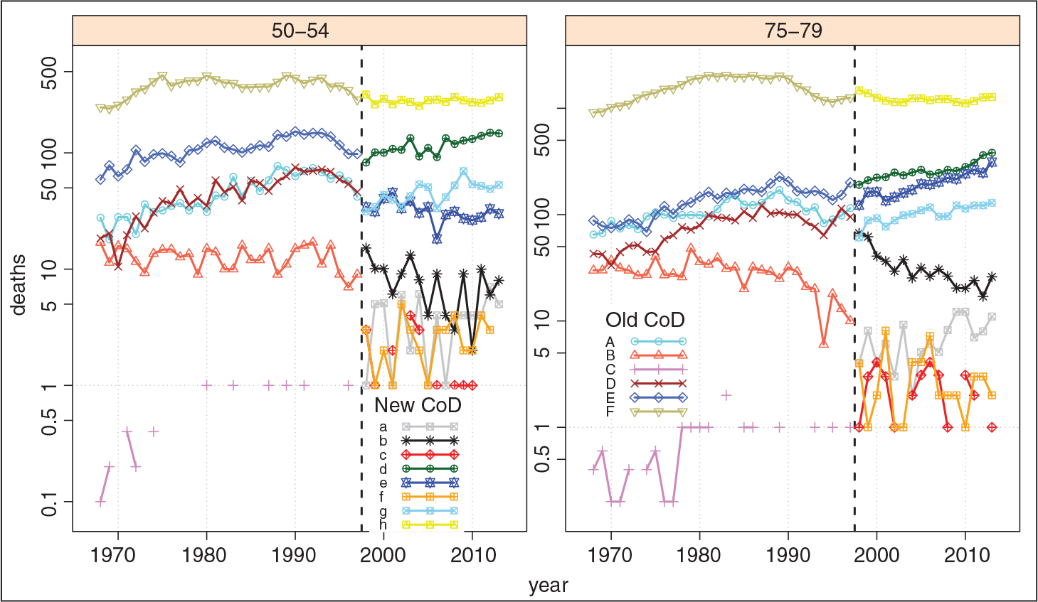
The CoDs in this dataset belong to the same group of malignant neoplasms (they are in the same association, as we say). Therefore, we can assume that all deaths due to the old CoDs would have been classified within the new CoDs, if the new classification had existed during the first period. The aim is to reconstruct coherent mortality trends over both periods in accordance with the new classification, that is, to redistribute deaths that occurred in the first period across the new CoDs.
Changes in medical practices can also lead to specific irregularities in a mortality time series by CoD. However, we will assume that disruptions in the revision year are solely due to changes in the official classification, without considering variations in coding practices arising during the same year. This is a reasonable assumption, since it considers the only certain and measurable events in cause-specific mortality series, allowing a statistical treatment of the problem. Other changes that occur during the year of transition will be then regarded as part of the revision process, and known irregularities in other years will have to be treated separately.
As mentioned, all possible exchanges across CoDs in the two revisions are defined in a correspondence table. This table can be succinctly written as a Boolean
Medical knowledge and a detailed understanding of the changes between two ICD revisions are necessary to create a correspondence table. In our German example, we used information provided by Pechholdová (2009), and we thus consider
Equation (2.1) informs us, for example, that counts belonging to the old CoD
Given the information in (2.1), we propose a method to estimate the so-called transition coefficients: These are proportions of counts in the categories of the old CoD coding that will be re-classified into the new CoD categories. Each age group may have its own transition coefficients.
We maintain the assumption made by Meslé and Vallin (1996) and later retained in other studies on reconstruction of mortality series by CoD (Pechholdová, 2009; Grigoriev et al., 2012; Pechholdová et al., 2017): The proportions across the old CoDs are equal in the two years right before and after the change in CoD coding. In our West German example, this means that proportions of counts classified as [A, B, ... , F] in 1997 are equal to the proportions of expected counts classified as [A, B, ... , F] in 1998. These expected counts are the proportions of the observed total death counts (per age-group) in 1998 in case they were classified still according to the old CoD scheme. Estimation will thus be based on death counts from the last year of the old classification and from the first year of the new classification.
For the complete reconstruction of cause-specific mortality series, we fix the estimated transition coefficients for the entire old period and redistribute all death counts in the old CoDs across the new CoDs. As a result, mortality trends in the old period (but expressed in the new CoD coding) will depend solely upon the actual trends among old CoDs.
In this section, we will build up our model and present the associated procedure for estimating the transition coefficients. We will start from the simple setting where all ages share the same transition coefficients. We will then generalize this approach to coefficients that may vary over ages, but in a smooth manner.
Constant transition coefficients over ages
The simplest assumption is to disregard age and redistribute the total number of deaths. Though relatively unrealistic, this first approach mirrors the conventional method in Meslé and Vallin (1996) and Pechholdová (2009), and it lays the groundwork for further steps.
Within this one-dimensional setting, we work with two vectors of death counts in the transition years. We denote with v = (v1, ... , vi, ... , vm)′ the observed deaths in the first year of the new revision. The vector z = (z1, ... , zj, ... , zn)′ defines the observed death counts in the last year of the old classification.
The requirement that the relative distribution of the causes of death should be the same in the two transition years can be expressed either in the new or in the old CoD coding. In the following, we express the observed proportions in the CoD categories in the old classification (

By assuming the same distribution among old CoDs in the transition years, we would expect that the total number of deaths observed in the first year of the new classification,

in case they still would have been categorized according to the old scheme. We denote the vector of these expected counts by

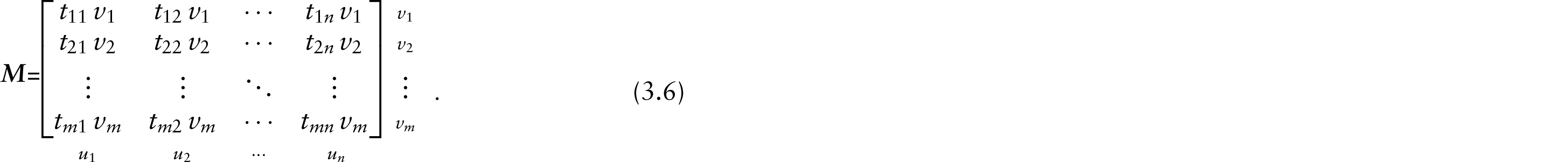
The matrix of transition coefficients

Each element
For a matrix T of transition coefficients and observed numbers of death v = (v1, ... , vm)′ in the first year of the new classification, the multiplication

gives the

with u as defined in Equation (3.2). In other words, we are looking for transition coefficients
Estimating proportions and working within a given association where death counts are fully exchanged, two conditions must be fulfilled.
Transition coefficients must be between 0 and 1. An estimated transition coefficient equal to 0 implies the removal of a link between an old and new CoD, even though it was assumed to be present in the correspondence table in All deaths in the first year of a new revision need to be redistributed according to the old classification, that is,
For a single age group, we could immediately simplify this equation to

Alternatively, the goal stated in (3.5) and condition 2 can be viewed as a way to fill a matrix with prescribed row and column sums, and where entries are functions of the unknown transition coefficients:
Whereas sums over rows concern observed death counts, column sums concern expected deaths based on the equal proportionality assumption. Constraints associated with row sums will thus be more stringent within our estimation procedure.
Equation (3.5) can be translated into a least-squares optimization problem. We denote with

where the full design matrix

By combining minimization in (3.7) and the previously presented conditions, we can treat the whole system as a QP problem

where

The condition that tij ϵ[ϵ, 1] is expressed in the first two constrained matrices and vectors:

Condition 2 about row sums is incorporated into the system by:

While introduced as equality, this condition was incorporated in the previous estimation procedure as a series of inequality constraints. We opted for this formulation since, for specific data and for transition coefficients bounded between
Given information about the presence of possible exchanges between causes expressed in the correspondence table
Note that both the design matrix
In particular, it could happen that, given a specific
As presented, the model has more unknown transition coefficients than observed independent marginals. Consequently, the associated system will have infinitely many solutions. We thus need to introduce additional information in order to solve an ill-posed problem and select one of the equally optimal solutions. To ensure a unique solution, one could employ a simple ridge penalty approach that penalizes the squared norm of
To illustrate this approach, we take an
Among infinite solutions from the constrained system in (3.8), we will favour estimated coefficients, which satisfies the following condition:

with,
We can express all conditions for all transition coefficients in a single matrix as follows:

and incorporate this additional constraint within (3.8) through a small regularization parameter. κr The QP problem becomes:

where

As before, we can remove all elements in
In other words, among all possible solutions given by (3.8), we select the transition coefficients that maintain an internal proportion over rows and columns similar to the observed proportions at the marginal level in M.
Whereas the constraints BÄ ≥ b are used to force all solutions within the [ϵ, 1] interval and to guarantee known sums over rows in (3.6), the penalty terms Pr and pr act ‘gently’ to lead all equally possible solutions, in terms of the residual sum of squares, towards a better internal proportionality. The value of κr is then selected to be rather small. Here, we use κr = 10-6.
Regarding the estimation approach, we have used the dual method of Goldfarb and Idnani (1983) implemented in the
Applied to the total number of deaths over the age dimension, the approach can be adapted for every single age group, independently estimating series of tijk for each age group k = 1, ... , ω. Alternatively, we can construct a system in which all tijk over
In this setting, we make use of the matrices of death counts from the last year of the old classification Z = (zjk) and from the first year of the new classification V = (vik). We can thus compute the matrix of expected death counts across old CoDs and age groups for the first year of new revision:

In two dimensions, the response in the constrained optimization problem is matrix

where

Associated constraint vector bs is given by bS = -

Concerning the regularization components,

with
By applying (3.10) with these generalized elements, we simultaneously obtain transition coefficients for each possible link and for all age groups, independently considered. Estimation results are thus identical to those obtained by treating each age group separately using the procedure presented in Section 3.1.
On the one hand, this approach is a straightforward extension over age of the conventional method, though embedded in a mathematical structure that routinely allows estimation of the coefficients. On the other hand, such generalization does not account for the continuous behaviour of mortality changes over age, that is, redistribution between CoDs in neighbouring age groups should not differ excessively. In other words, in the absence of specific and usually well-understood irregularities, a smooth change of the estimated transition coefficients over age groups is a reasonable and flexible approach.
Moreover, wiggly behaviour of tijk over
It is thus reasonable to assume that underlying trends of tijk vary smoothly over ages. We introduce this smooth behaviour to the series of coefficients by adding a roughness penalty in (3.10):

The term

where
The smoothing parameter
Moreover, as will be shown in Section 4, differences between reconstructed series based on unsmooth and smooth transition coefficients are negligible, at least for the considered time horizons. The smoothing parameter can thus be tuned subjectively to incorporate a certain amount of smoothness, sufficient to prevent inconsistent trends in long-term reconstructed age- and cause-specific mortality series. The choice of
Three different assumptions could be made with respect to the changes of tijk over k: a common transition coefficient for all ages (cf. Section 3.1), coefficients independently estimated for each age (using λ = 0 in (3.12)) and a smooth change of the estimated transition coefficients over age groups.
Furthermore, a fourth option might be applicable: assuming constant transition coefficients over ages by selecting d = 1 in Dd and extremely large smoothing parameters: λ = 108. In this way, we approach the limit for strong smoothing, which is a polynomial of degree
As in the one-dimensional setting, we remove from all the components of the constrained optimization problem in (3.12), all elements corresponding to
Malignant neoplasms in Germany
Figure 2 presents the estimated transition coefficients over age groups, arranged as in the correspondence table
Estimated transition coefficients τ, ‰. Constant coefficients over age groups. Association for some malignant neoplasms (cf. Section 2)
Estimated transition coefficients τ, ‰. Constant coefficients over age groups. Association for some malignant neoplasms (cf. Section 2)
Note that when we assumed a single coefficient for all age groups, some transition coefficients are necessarily estimated equal to definite values: see tcB, tcC, teF, thD, thE, thF in Table 1. Consequently, differences between the proposed regularization and ridge regression are visible only for the remaining
In Figure 2, smooth transition coefficients are portrayed by solid lines. For this example, we use a smoothing parameter λ = 106. Most of the time the smooth estimates approximate the age-independent coefficients, especially when more death counts are involved in the age- and cause-specific link. The ‘size’ of these links is correlated with the size of the circles in Figure 2. This information helps to explain why the smooth estimates are not exactly smooth correspondents of the age-independent ones: when few deaths are involved, enforcing smoothness is preferable at the cost of small errors in terms of age-specific marginal sums in the correspondence matrix (3.6).
In order to assess the performance of each approach, we compute the total absolute loss in death counts, that is, we sum the absolute differences between estimated and observed/expected marginals in (3.6). Whereas smooth transition coefficients lead to an error of only 1.8% with respect to the overall sample size, using constant coefficients over ages brings an error of 2.6%. Age-independent transition coefficients with wiggling behaviour leads to a relative error of 0.2%. This last value is due to the fact that, for some ages, coefficients are estimated within the region expressed by inequality constraints
The left panel of Figure 3 presents the reconstructed death series for the age group 75–79 and for all three approaches. Note that estimating coefficients based solely on data in this age group (dashed-line) may lead to unreasonable outcomes when few counts are involved in the reconstruction. Moreover, for certain CoDs, disruptions in the year of revision are noticeable when a constant coefficient is estimated for all ages (see dotted lines for CoD
The development of CoD
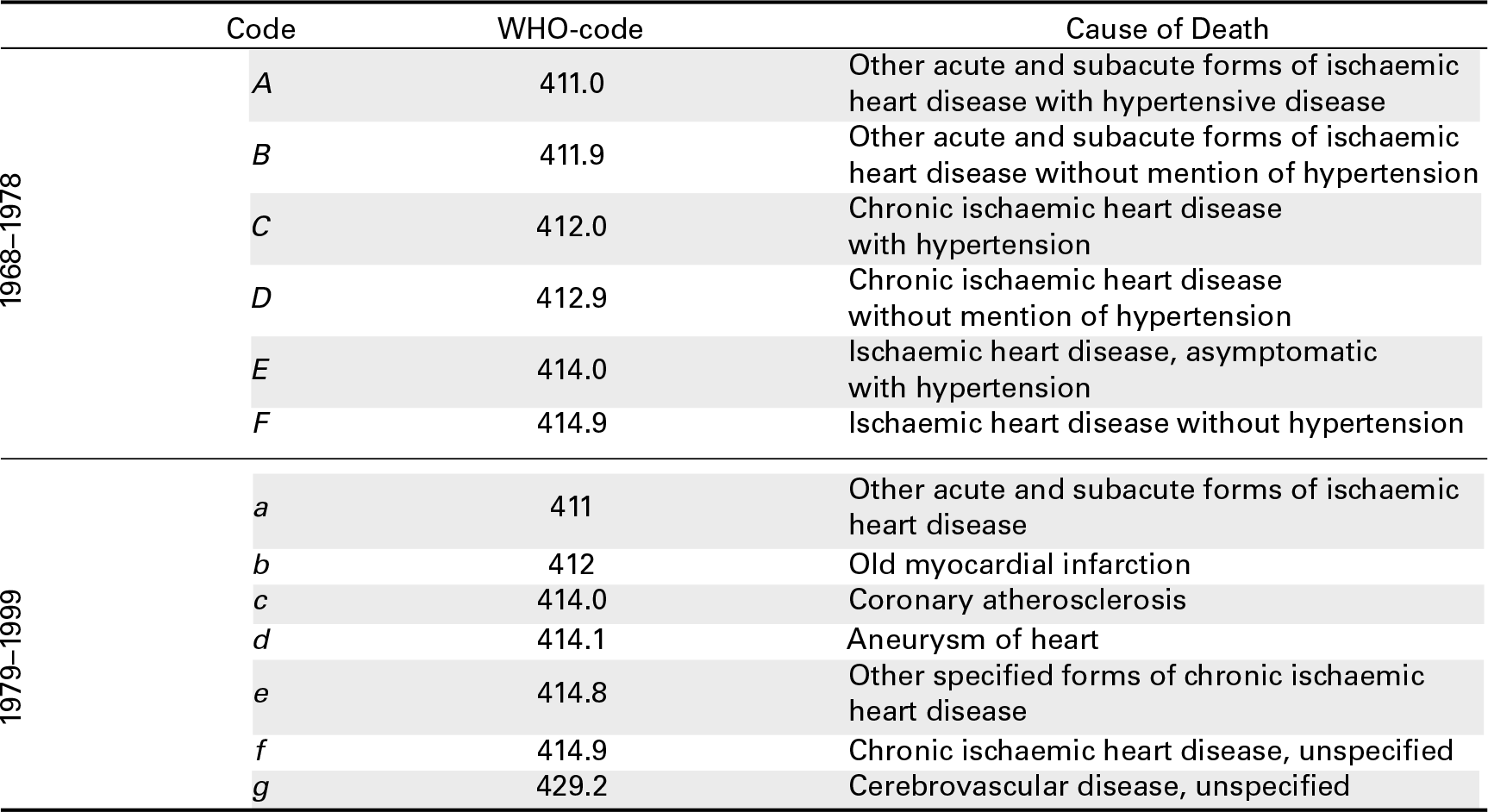
In this section, we present the results for an association of some major heart diseases in France. A complete list of items with their original names is given in Table A.2. We start from ages 30–34, and 100+ represents the last open age group. Here, we analyse data from two ICD classifications: ICD-8, which was in use from 1968 to 1978, and ICD-9, which was in use from 1979 to 1999.
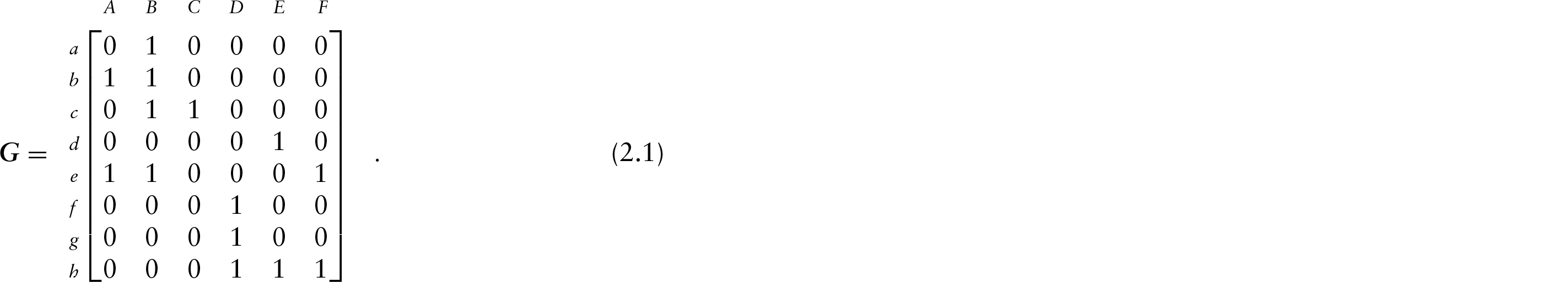
A crucial input for estimating transition coefficients is the correspondence table G, which describes possible exchanges across CoDs between the two classifications. Here G, was provided by Meslé and Vallin (1996), and it is given by
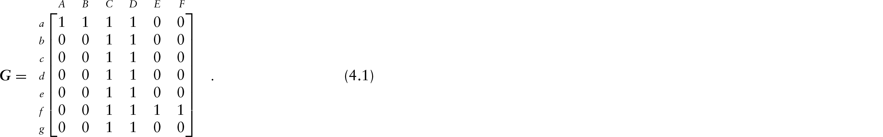
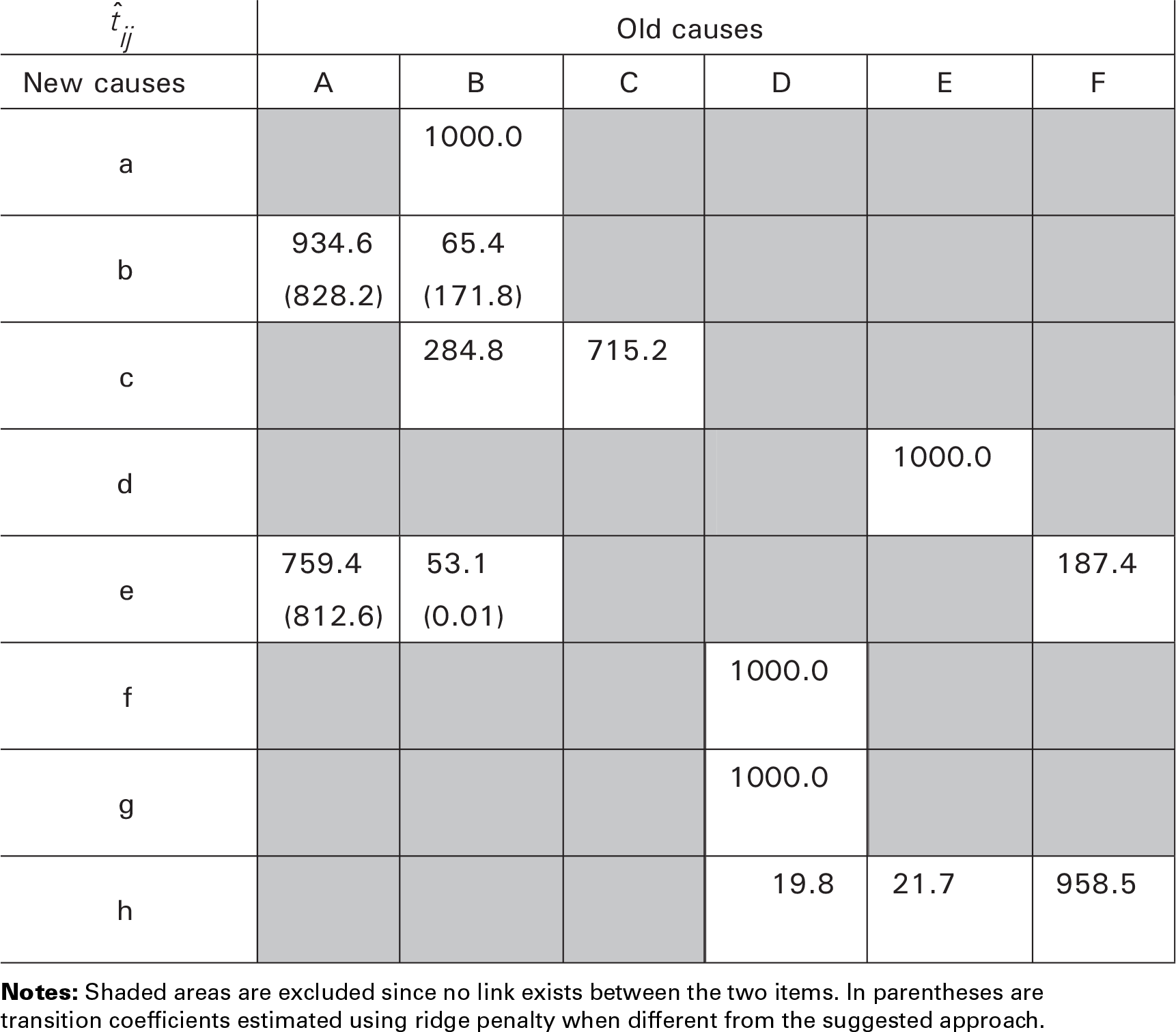
Similar to the German example, we can build up a system of equations as in (3.10). Table 2 shows the outcomes for this group of heart diseases in France at the introduction of ICD-9 in 1979, in which we summed data over all ages. Note that due to the proportionality constraints in (3.9) and the structure of (4.1), our approach will favour equal transition coefficients for third and fourth columns. For comparison, Table 2 shows the estimation using a ridge penalty approach (in parentheses) and the transition coefficients computed manually for this association by (Meslé and Vallin, 1996) (p. 79; in square brackets).
Estimated transition coefficients τ, ‰. Constant coefficients over age groups. Association for major heart diseases
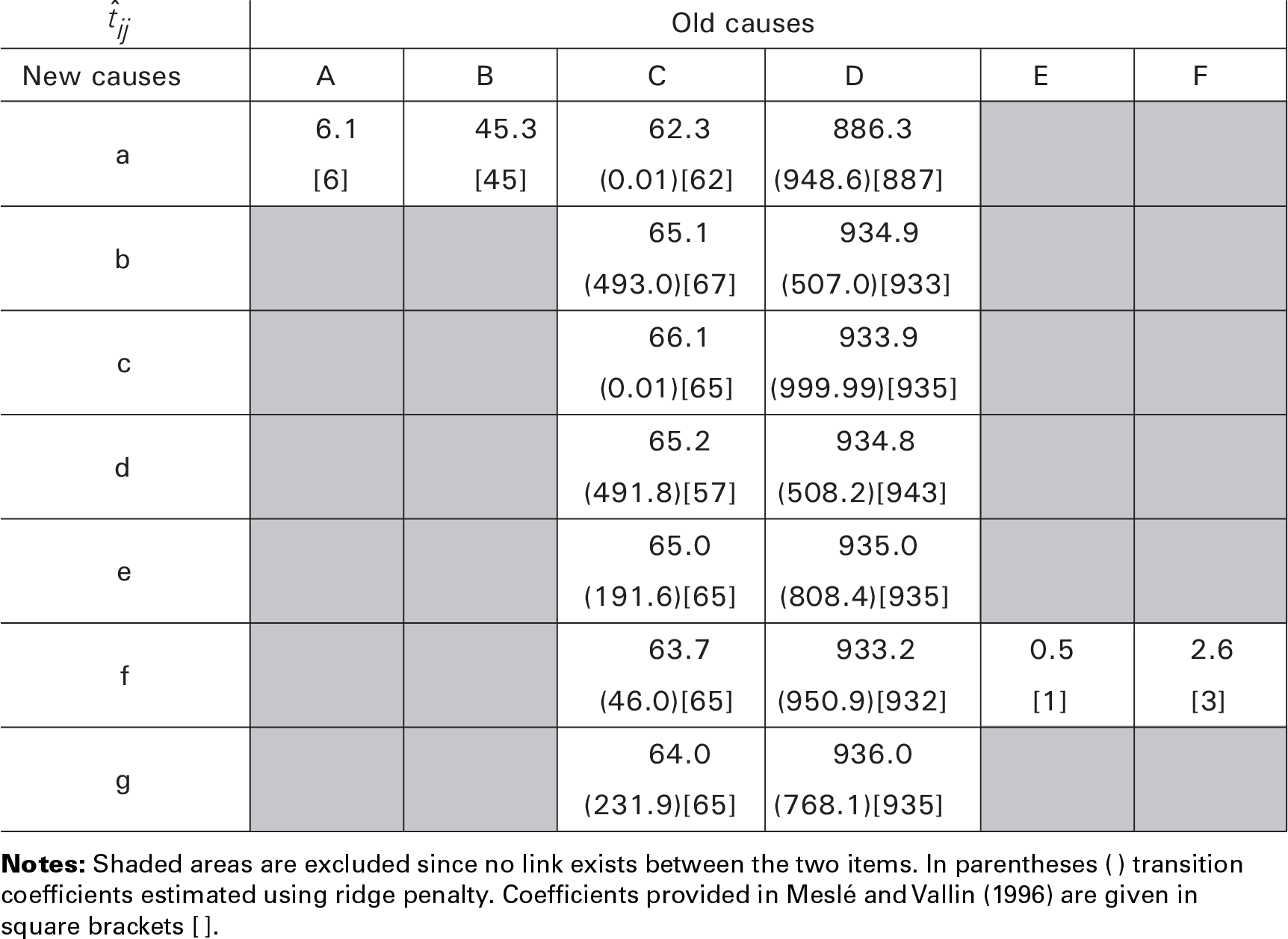
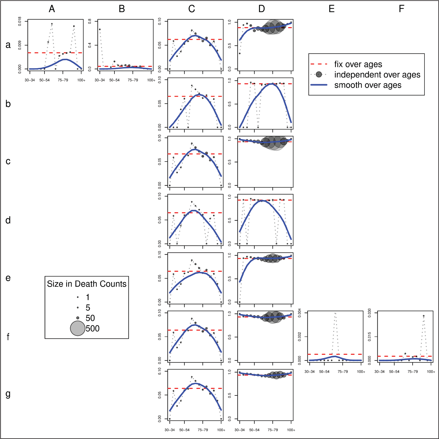
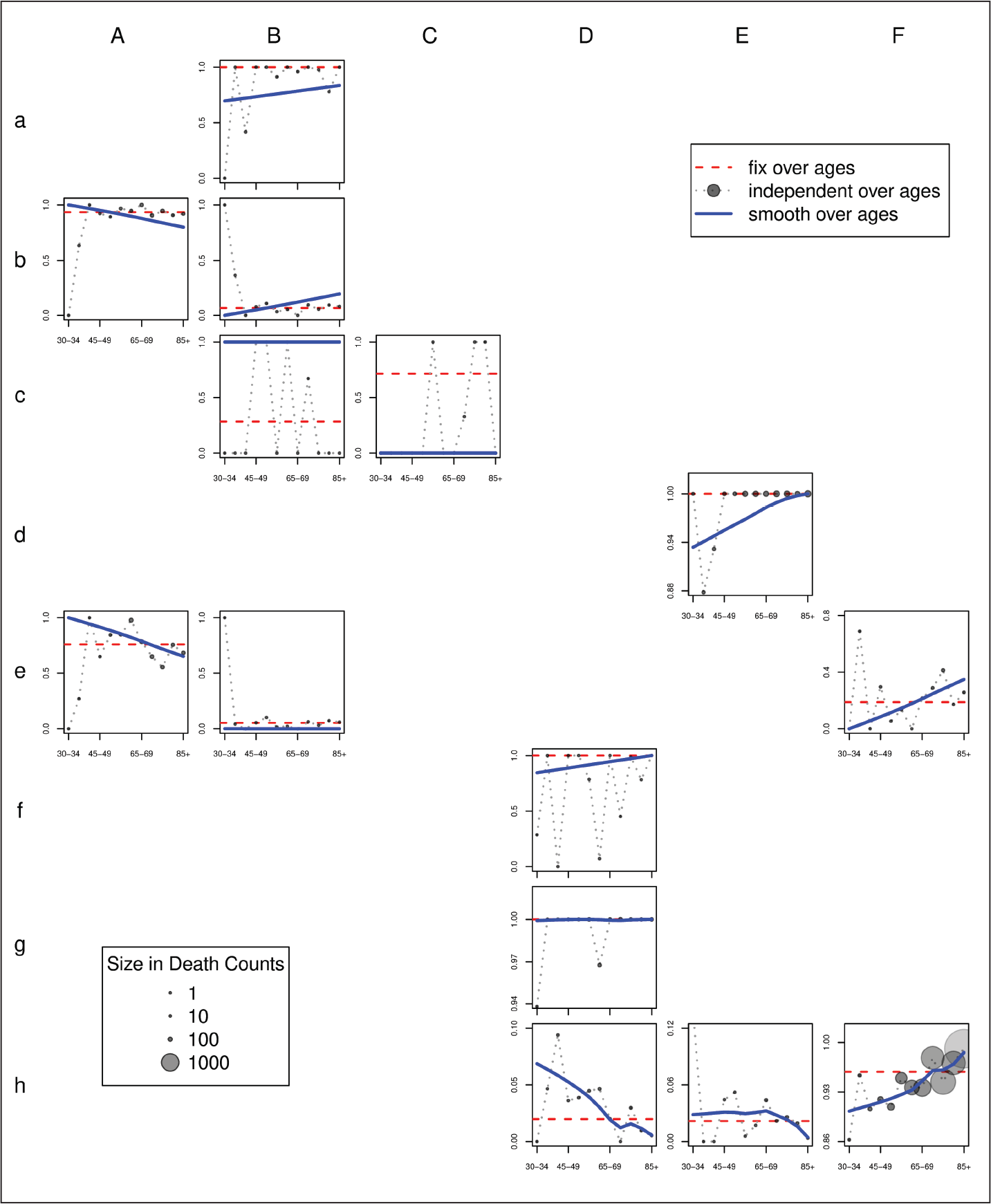
Figure 4 shows the outcomes for this group of heart diseases in France at the introduction of ICD-9 in 1979. When we summed data over all ages, the presented regularization penalty provided a means to extract the most suitable solution based on our assumptions (see dashed horizontal lines in Figure 4). The fluctuating dotted lines in Figure 4 illustrate the outcomes of an age-independent estimation of transition coefficients. As in the previous example, the size of the circles represents the number of deaths in each cause-age combination based on the age-independent estimation of tijk. Finally, the solid curves portray smooth estimated transition coefficients over age. As expected, these curves closely follow cause-age combinations with more deaths.
In terms of total absolute losses in death counts, assuming constant coefficients for all ages leads to an error of 2.3%. A better outcome is obtained when we smooth the transition coefficients, that is,absolute losses equal to 1.9%. When the estimation procedure is applied at each age independently, coefficients are always so that

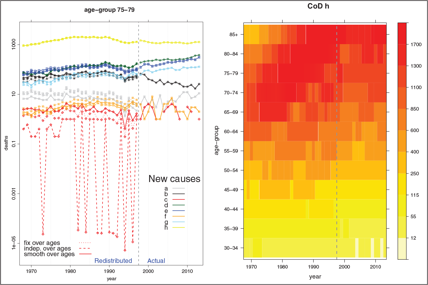
Figure 5 presents the final outcomes obtained using the estimated transition coefficients to reconstruct coherent mortality series by CoD. The left panel shows reconstructed series of death counts for a specific age group (75–79) for the three different assumptions. As mentioned, outcomes due to smooth and age-independent transition coefficients are very much alike (solid and dashed lines). Exceptions are visible for CoDs with low death counts. Redistributing death counts for each age group by using transition coefficients estimated for all ages can lead to unsatisfactory disruptions in the year of transition (see dotted lines). The right panel in Figure 5 presents a shaded contour map of death counts for a specific CoD (
Changes in the classification of causes of death lead to disruptions in mortality series by CoD. Therefore, a comprehensive analysis of mortality trends involves the important task of reconstructing series that coherently consider the CoD dimension. An important step in this task is the computation of transition coefficients, that is, the proportions of deaths moving from old to new CoDs in the year of transition between classifications.
The first step in the reconstruction procedure is the identification of associations: independent groups of old and new CoDs that fully exchange their death counts in the transition years, however, with possible exchanges, fully or partially, between causes in the association. The construction of these associations is based on medical content in both revisions, and here they are considered a fixed input. Often these associations involved several CoDs, and estimation of transition coefficients is not evident and unique. Conventional approaches rely on manual computation of these coefficients, mainly based on experience acquired in the field. Moreover, this procedure is commonly performed for all age groups together and ex-post adjustments are needed for a more coherent reconstruction in each age group.
In this article, we propose a model to routinely estimate transition coefficients. Starting from basic assumptions on possible exchanges across causes of death between two revisions, we describe the problem as a least-squares optimization with inequality constraints. A QP approach allows us to estimate these coefficients within an interval, which is needed since the unknowns are proportions. Moreover, as we are dealing with an ill-posed problem, we propose a specialized regularization to mirror the logic used by researchers in the field.
Three possible options are provided in the estimation of transition coefficients. First, simple solution treats all age groups together, and the same coefficient is estimated for all ages. The second and more generalized approach assumes a series of transition coefficients that is estimated for each age group independently. The final and more reasonable compromise assumes smooth behaviour of the coefficients over age groups. A roughness penalty is introduced to incorporate this assumption in a system that simultaneously deals with all age groups.
We present two applications whose outcomes are more than satisfactory. First, we considered an association with specific malignant neoplasms in Germany and the disruptions due to change between ICD-9 and ICD-10 in 1997–1998. Estimated transition coefficients capture the levels of exchange across old and new CoDs. Associated reconstructed mortality series clearly show no disruptions based on visual examination. As a second example, we used French data on major heart diseases over the revisions ICD-8 and ICD-9. Disruptions are due to change in the classification in 1978–1979. Outcomes here are equally good. Further analysis to statistically assess the presence of disruptions in cause-specific mortality series goes beyond the scope of this article, and it was presented elsewhere (Camarda and Pechholdová, 2014).
The assumption that the proportions of counts by CoD are equal as in the years of classification revision, though reasonable, needs further consideration. In the current version of the model, we weaken this assumption in the estimation procedure if there is good reason to believe that the correspondence table is correct. Alternatively, we plan to extend the model assuming a smooth change of the proportions over the new period and back-forecasting these proportions in the last year of the old classification. For modelling proportions, Compositional Data Analysis seems to be a reasonable methodology to employ in this context (Pawlowsky-Glahn and Buccianti, 2011). However, this extension will only modify the way of obtaining the vector of expected deaths (
Sometimes the presence of possible links between old and new CoDs is unclear within certain associations. Additional regularization might be envisaged to select possible exchanges between CoDs. Regression methods with regularization by the Lasso and the Elastic Net (Tibshirani, 1996; Zou and Hastie, 2005) seem good candidates for extending our approach in this direction.
Finally, we want to point out that the proposed method has been used extensively in the recently established Human Cause-of-Death Database (2018), a collection of coherent time series of cause-specific mortality for 16 countries. The suggested approach can be extended to other contexts where time series are disrupted for known reasons, for example, series with historic border changes.
Acknowledgments
I would like to show my gratitude to Paul Eilers for sharing his pearls of wisdom with me during the preparation of the manuscript. I am deeply grateful to Jutta Gampe for many helpful comments on earlier versions of this article, both statistical and stylistic. The credit for introducing me to the field of cause-of-death analysis goes to Markéta Pechholdová and France Meslé.
Declaration of conflicting interests
The author declared no potential conflicts of interest with respect to the research, authorship and/or publication of this article.
Funding
This work was supported by the ‘AXA project on Mortality Divergence and Causes of Death’ and ‘Project ANR-12-FRAL-0003-01 DIMOCHA’.
Appendix
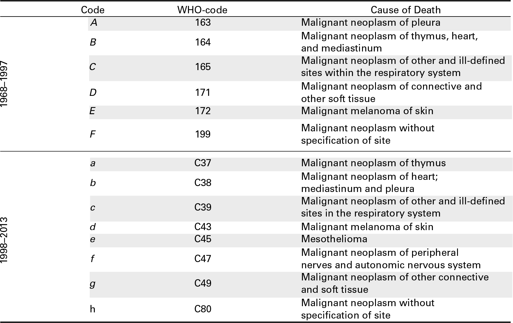
For ease of presentation, in the article, we use upper- and lower-case letters for designating CoDs within a certain association. In this Appendix, we list the original corresponding names as provided by theWorld Health Organization. Table A.1 shows the items for specific malignant neoplasms in West Germany used for the ICD-9 and ICD-10 classifications during the period 1978–1997 and 1998–2013, respectively. These causes were used to illustrate the proposed model and in Section 4.1 to show the outcomes of an application. Table A.2 presents the original CoDs employed in Section 4.2 for a specific group of heart diseases in France for ICD-8 (until 1978) and ICD-9.
Cause of death for specific malignant neoplasms inWest Germany from 1968 to 2013 during two ICD revision periods: ICD-9 and ICD-10. Original WHO codes are also provided
Cause of death for specific heart diseases in France from 1968 to 1999 during two ICD revision periods: ICD-8 and ICD-9. OriginalWHO codes are also provided