Semiparametric regression analysis of multivariate doubly censored data

Abstract

This article discusses regression analysis of multivariate doubly censored data with a wide class of flexible semiparametric transformation frailty models. The proposed models include many commonly used regression models as special cases such as the proportional hazards and proportional odds frailty models. For inference, we propose a nonparametric maximum likelihood estimation method and develop a new expectation–maximization algorithm for its implementation. The proposed estimators of the finite-dimensional parameters are shown to be consistent, asymptotically normal and semiparametrically efficient. We also conduct a simulation study to assess the finite sample performance of the developed estimation method, and the proposed methodology is applied to a set of real data arising from an AIDS study.

Keywords

Multivariate doubly censored data Maximum likelihood estimation frailty model semiparametric efficiency expectation–maximization algorithm

1 Introduction

Doubly censored data arise frequently in many scientific areas including clinical trials, demographical investigations, epidemiology studies and tumorigenicity experiments (Gehan (1965); Chang and Yang (1987); Chang (1990); Mykland and Ren (1996); Zhang and Jamshidian 2004). For such data, the outcome variable of interest can only be observed accurately within a certain interval, and outside this interval, the outcome variable is either left censored or right censored rather than observed exactly. An example of such data is given by an AIDS clinical trial involving the measurement of the plasma HIV-1 RNA level, which is usually done by the use of the NucliSens assay that is highly unreliable if the RNA level is below 400 or above 750 000 per millilitre of plasma. In other words, one can obtain the exact plasma HIV-1 RNA level if it is between 400 and 750 000, and otherwise, the plasma HIV-1 RNA level is either left censored by 400 or right censored by 750 000. That is, we only have doubly censored data on RNA level or value. If the outcome variable is a failure time such as the chronic Hepatitis B virus (HBV) infection time, then the left censoring occurs when a subject has already been infected with the HBV before the entry of the study and the right censoring occurs when the subject has not yet experienced the HBV infection by the end of the study. Multivariate doubly censored data mean that there exist several correlated outcomes of interest and only doubly censored data are available for each outcome variables.

It is worth noting that in the literature, the terminology doubly censored data may sometimes be used to denote another type of censored data in which the outcome variable of interest is defined as the elapsed or gap time from an initial event to a subsequent event, and the occurrences of both events may suffer interval censoring (Sun (1995); Sun (2006); Komárek and Lesaffre 2006). A typical example of such data occurs in an AIDS cohort study in which the interest lies in investigating the effect of covariates on the AIDS incubation time defined as the elapsed time from the infection of human immunodeficiency virus (initial event) to the onset of AIDS (subsequent event). Note that the data structures of such data and the data discussed above are quite different and they also require different statistical techniques for their analyses. In the following, we will focus on the first type of doubly censored data.

Many methods have been proposed for the analysis of univariate doubly censored data, especially for their regression analysis (Zhang and Li (1996); Cai and Cheng (2004); Kim et al. (2010); Kim et al. (2013); Li et al. 2018). For example, Cai and Cheng (2004), Kim et al. (2013) and (Li et al. 2018) studied the fitting of the linear transformation model, the proportional hazards model and a class of semiparametric transformation models to such data, respectively. In general, regression analysis of doubly censored data is much more challenging than that of right-censored data due to the presence of left-censorship. Under this situation, the classical partial likelihood approach for the proportional hazards model with right-censored data is no longer applicable and one has to deal with or estimate both infinite-dimensional nuisance parameter and finite-dimensional regression parameters together.

For the analysis of multivariate censored data, one of the main challenges is how to deal with the correlation of different outcome variables. For this, one of the most commonly used approaches is the marginal model-based approach, which relies on the working independence assumption and can give consistent estimates if the marginal models are correctly specified (Goggins and Finkelstein (2000); Wei et al. 2015). Another commonly used approach is the joint modelling approach which characterizes the relationship of the correlated outcome variables by using either the copula or the frailty model (Wang and Ding (2000); Sun et al. (2006); Wang et al. (2015); Wen and Chen (2015); Su and Wang (2016); Hu et al. 2017). The former models the joint cumulative distribution or survival function of the correlated outcome variables with some copula function, while the latter uses some latent variables or frailties to link the marginal hazard functions of different failure times together. With the latter approach, for estimation, the expectation–maximization (EM) algorithm is commonly employed by treating the latent variables as observable.

In the following, we will employ the latter approach and present a wide class of semiparametric transformation frailty models, which is quite flexible and includes many commonly used models such as proportional hazards and proportional odds frailty models as special cases. For inference, we consider the nonparametric maximum likelihood method and develop a novel EM algorithm with the use of some Poisson variables. In particular, in the E-step of the algorithm, we propose to jointly employ probability integral transformation and Gaussian–Hermite quadrature techniques to calculate the conditional expectations with respect to the frailties, which is reliable and can apply to the general situation as discussed below.

The rest of this article is organized as follows. In Section 2, we introduce the data structure and the models, and present the corresponding likelihood function. Section 3 discusses the proposed nonparametric maximum likelihood estimation procedure and the development of a novel EM algorithm. The asymptotic properties of the proposed estimators are established in Section 4. In Section 5, we conduct a simulation study to evaluate the finite sample performance of the proposed method. In Section 6, we illustrate the usefulness of the proposed method with an AIDS dataset, and Section 7 includes some discussion and concluding remarks.

2 Data, models and the likelihood function

Consider a study that involves $n$ independent subjects and each subject can experience $K$ different, correlated events. Let $T_{ik}$ denote the outcome variable of the $k$ th event for the $i$ th subject, $k = 1, \dots, K$ , $i = 1, \dots, n$ . As mentioned above, such multivariate data occur commonly in many fields, and one example is given by the AIDS Clinical Trials Group $181$ study (Goggins and Finkelstein (2000); Zhou et al. 2017), which investigated whether the baseline CD4 cell count is predictive of the cytomegalovirus (CMV) shedding in both blood and urine. In the following, suppose that only the doubly censored data are available on the $T_{ik}$ ’s. That is, for each $i$ and $k$ , $T_{ik}$ can only be observed exactly within the window $(L_{ik}, R_{ik}]$ , where $L_{ik} < R_{ik}$ , and the observed information for each subject is given by ${{\tilde{T}}_{ik}, Δ_{1 ik}, Δ_{2 ik}, X_{ik} (\cdot)}$ . Here, ${\tilde{T}}_{ik} = max {L_{ik}, min (T_{ik}, R_{ik})}$ , $Δ_{1 ik} = I (T_{ik} \leq L_{ik})$ , $Δ_{2 ik} = I (L_{ik} < T_{ik} \leq R_{ik})$ , $I (\cdot)$ denotes the indicator function, and $X_{ik} (\cdot)$ is a $d$ -dimensional vector of possibly time-dependent covariates. It is easy to see that $Δ_{1 ik} + Δ_{2 ik} = 0$ if $T_{ik}$ is right censored.

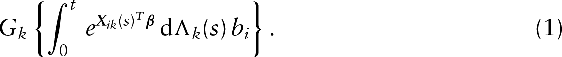
In the following, we will consider the frailty model-based approach and assume that there exists a latent variable $b_{i}$ for each subject $i$ and the $b_{i}$ ’s follow the density function $p (\cdot | γ)$ , which has mean one and is known up to the unknown parameter $γ$ . Also assume that given the covariate process ${X_{ik} (s), s < t}$ and $b_{i}$ , the cumulative hazard function of $T_{ik}$ has the form

G_{k} \{\int_{0}^{t} e^{X_{ik} (s)^{T} β} d Λ_{k} (s) b_{i}\} .

(1)

In the above, $Λ_{k} (t)$ denotes an unknown increasing baseline cumulative hazard function, $β$ is a $d$ -dimensional vector of regression parameters and $G_{k}$ is a prespecified function that is also increasing. Furthermore, it will be assumed that given $b_{i}$ , $T_{i 1}, \dots, T_{iK}$ are independent, a commonly used assumption under the framework of frailty models (Zeng et al. (2008); Zhou et al. 2017).

The class of models (1) is quite flexible and encompasses many commonly used models as special cases. For example, we can obtain the proportional hazards frailty model by letting $G_{k} (x) = x,$ and it gives the proportional odds frailty model when $G_{k} (x) = \log (1 + x)$ . If the covariates are time-invariant, then it reduces to the linear transformation model

log Λ_{k} (T) = - X_{ik}^{T} β - log (b_{i}) + ε_{k},

where $ε_{k}$ is a random term with a known distribution function $1 - exp {- G_{k} (exp (\cdot))}$ . Note that among others, Zeng et al. (2008) and Zeng et al. (2009) used the similar transformation frailty models as above for the analysis of multivariate right-censored data.

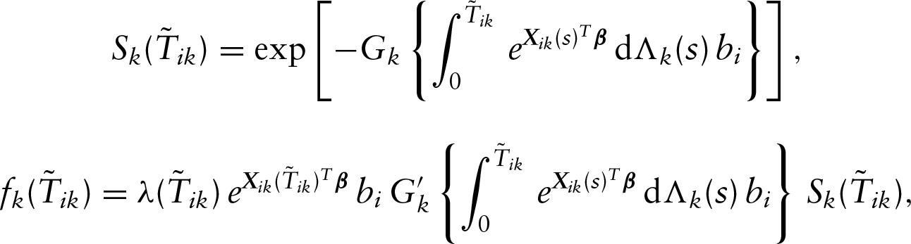
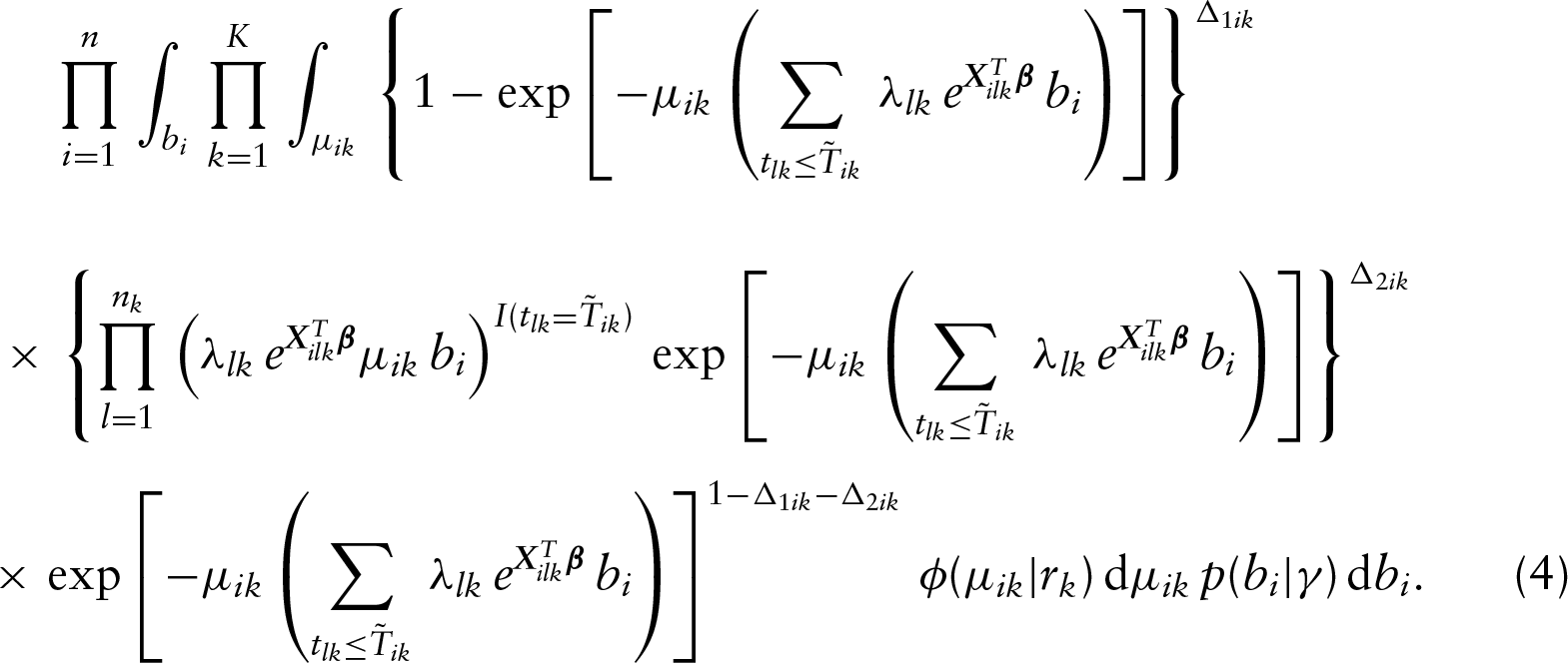
Let $f_{k}$ and $S_{k}$ denote the density and survival functions of the $k$ th outcome variable, respectively. Then under the conditional independence assumption between $T_{ik}$ and $(L_{ik}, R_{ik})$ given $X_{ik} (\cdot)$ and $b_{i}$ , the observed data likelihood function takes the form

\prod_{i = 1}^{n} \int_{b_{i}} \prod_{k = 1}^{K} {\{1 - S_{k} ({\tilde{T}}_{ik})\}}^{Δ_{1 ik}} f_{k} ({\tilde{T}}_{ik})^{Δ_{2 ik}} S_{k} ({\tilde{T}}_{ik})^{1 - Δ_{1 ik} - Δ_{2 ik}} p (b_{i} | γ) d b_{i},

(2)

where

\begin{matrix} S_{k} ({\tilde{T}}_{ik}) = exp [- G_{k} \{\int_{0}^{{\tilde{T}}_{ik}} e^{X_{ik} (s)^{T} β} d Λ_{k} (s) b_{i}\}], \\ f_{k} ({\tilde{T}}_{ik}) = λ ({\tilde{T}}_{ik}) e^{X_{ik} ({\tilde{T}}_{ik})^{T} β} b_{i} G_{k}^{'} \{\int_{0}^{{\tilde{T}}_{ik}} e^{X_{ik} (s)^{T} β} d Λ_{k} (s) b_{i}\} S_{k} ({\tilde{T}}_{ik}), \end{matrix}

and $G_{k}^{'} (x) = d G_{k} (x) / d x$ . Note that the conditional independence assumption described above can be relaxed to the noninformative censoring assumption, meaning that the joint distribution of the $L_{ik}$ ’s and $R_{ik}$ ’s does not involve any unknown parameters in the class of models (1) for $T_{ik}$ (Scharfstein and Robins (2002); Siannis et al. 2005; Gómez et al. 2009).

For the estimation, it is obvious that a natural way is the direct maximization of the likelihood function (2). On the other hand, one can see that this would be very challenging and can be unstable due to the complex data structure and the existence of the nonparametric functions $Λ_{k} (t)$ ’s. Thus, in the following, we will develop an EM algorithm with the use of Poisson variables. A key advantage of the described data augmentation is that one only needs to maximize an objective function with a much simpler form in the M-step of the algorithm, which can also be easily implemented as seen below.

3 Maximum likelihood estimation and the EM algorithm

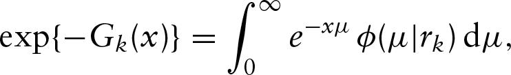
In this section, we will discuss the development of an EM algorithm for the maximization of the likelihood function given in (2). For this, first note that the transformation function $G_{k}$ can be derived as follows

exp {- G_{k} (x)} = \int_{0}^{\infty} e^{- x μ} ϕ (μ | r_{k}) d μ,

where $ϕ (μ | r_{k})$ is the density function of the frailty $μ$ with the known parameter $r_{k}$ . For example, we can obtain $G_{k} (x) = \log (1 + r_{k} x) / r_{k}$ , the logarithmic transformation function, if $ϕ (μ | r_{k})$ is the density function of a gamma random variable with mean one and variance $r_{k}$ . This suggests that one can convert the class of transformation frailty models (2) into the proportional hazards model with two sets of frailties Kosorok et al. (2004).

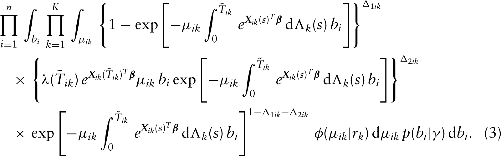
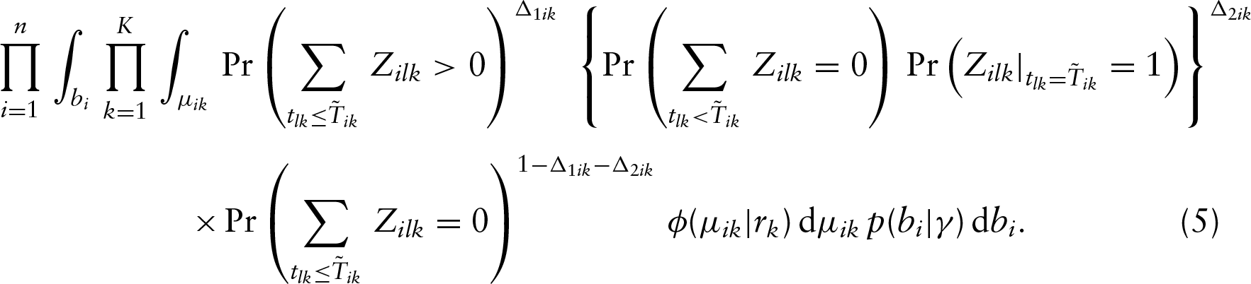
To develop the proposed EM algorithm, we will first describe the needed data augmentation. Let the $μ_{ik}$ ’s be the replicates of $μ$ above. Then the likelihood function given in (2) can be equivalently expressed as

\begin{matrix} \prod_{i = 1}^{n} \int_{b_{i}} \prod_{k = 1}^{K} \int_{μ_{ik}} {\{1 - exp [- μ_{ik} \int_{0}^{{\tilde{T}}_{ik}} e^{X_{ik} (s)^{T} β} d Λ_{k} (s) b_{i}]\}}^{Δ_{1 ik}} \\ \times {\{λ ({\tilde{T}}_{ik}) e^{X_{ik} ({\tilde{T}}_{ik})^{T} β} μ_{ik} b_{i} exp [- μ_{ik} \int_{0}^{{\tilde{T}}_{ik}} e^{X_{ik} (s)^{T} β} d Λ_{k} (s) b_{i}]\}}^{Δ_{2 ik}} \\ \times exp {[- μ_{ik} \int_{0}^{{\tilde{T}}_{ik}} e^{X_{ik} (s)^{T} β} d Λ_{k} (s) b_{i}]}^{1 - Δ_{1 ik} - Δ_{2 ik}} ϕ (μ_{ik} | r_{k}) d μ_{ik} p (b_{i} | γ) d b_{i} . \end{matrix}

(3)

For the infinite-dimensional function $Λ_{k} (t)$ , we propose to approximate it with a step function with non-negative jumps at all distinct uncensored observations and an additional set of left-censored observations of the $k$ th event, a subset of $\{{\tilde{T}}_{1 k}, \dots, {\tilde{T}}_{nk}\}$ with $Δ_{1 ik} = 1$ or $Δ_{2 ik} = 1$ . The aim of including left-censored observations in the support of $Λ_{k} (t)$ is to ensure the existence of the nonparametric maximum likelihood estimator, and for more details on this, one can refer to the Lemma 2.1 given in Su and Wang (2016) and the Corollary 5 given in Mykland and Ren (1996). We denote those distinct time points in ascending order by $t_{1 k}, \dots, t_{n_{k} k}$ with corresponding jump sizes $λ (t_{lk})$ for $l = 1, \dots, n_{k}$ . For notational simplicity, in the following, we denote $λ_{lk} = λ (t_{lk})$ and $X_{ilk} = X_{ik} (t_{lk})$ for $l = 1, \dots, n_{k}$ . Then the likelihood function $(3)$ becomes

\begin{matrix} \prod_{i = 1}^{n} \int_{b_{i}} \prod_{k = 1}^{K} \int_{μ_{ik}} {\{1 - exp [- μ_{ik} (\sum_{t_{lk} \leq {\tilde{T}}_{ik}} λ_{lk} e^{X_{ilk}^{T} β} b_{i})]\}}^{Δ_{1 ik}} \\ \begin{matrix} \times {\{\prod_{l = 1}^{n_{k}} {(λ_{lk} e^{X_{ilk}^{T} β} μ_{ik} b_{i})}^{I (t_{lk} = {\tilde{T}}_{ik})} exp [- μ_{ik} (\sum_{t_{lk} \leq {\tilde{T}}_{ik}} λ_{lk} e^{X_{ilk}^{T} β} b_{i})]\}}^{Δ_{2 ik}} \\ \times exp {[- μ_{ik} (\sum_{t_{lk} \leq {\tilde{T}}_{ik}} λ_{lk} e^{X_{ilk}^{T} β} b_{i})]}^{1 - Δ_{1 ik} - Δ_{2 ik}} ϕ (μ_{ik} | r_{k}) d μ_{ik} p (b_{i} | γ) d b_{i} . \end{matrix} \end{matrix}

(4)

Next, for the $k$ th event of the $i$ th subject, we introduce a set of independent latent variables ${Z_{ilk}}_{l = 1}^{n_{k}}$ , where $Z_{ilk}$ follows the Poisson distribution with mean $λ_{lk} e^{X_{ilk}^{T} β} μ_{ik} b_{i}$ . Then we find that the likelihood function $(4)$ can be rewritten as

\begin{matrix} \prod_{i = 1}^{n} \int_{b_{i}} \prod_{k = 1}^{K} \int_{μ_{ik}} \Pr {(\sum_{t_{lk} \leq {\tilde{T}}_{ik}} Z_{ilk} > 0)}^{Δ_{1 ik}} {\{\Pr (\sum_{t_{lk} < {\tilde{T}}_{ik}} Z_{ilk} = 0) \Pr (Z_{ilk} |_{t_{lk} = {\tilde{T}}_{ik}} = 1)\}}^{Δ_{2 ik}} \\ \times \Pr {(\sum_{t_{lk} \leq {\tilde{T}}_{ik}} Z_{ilk} = 0)}^{1 - Δ_{1 ik} - Δ_{2 ik}} ϕ (μ_{ik} | r_{k}) d μ_{ik} p (b_{i} | γ) d b_{i} . \end{matrix}

(5)

That is, we have re-expressed the likelihood function (4) with some Poisson variables, which is crucial and useful for the development of the following complete data likelihood function with a much simpler form.

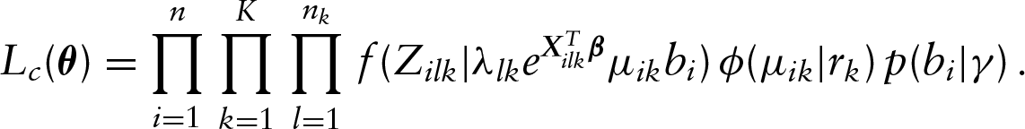
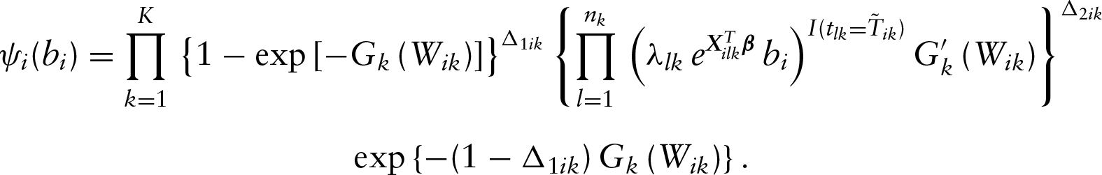
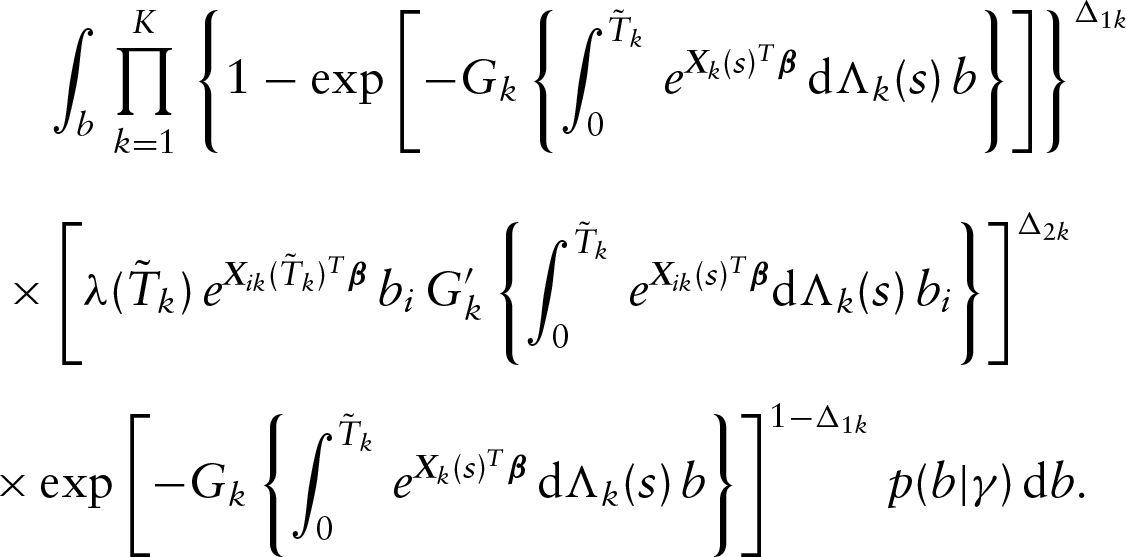
Let $f (Z_{ilk} | λ_{lk} e^{X_{ilk}^{T} β} μ_{ik} b_{i})$ be the density function of $Z_{ilk}$ with the parameter $λ_{lk} e^{X_{ilk}^{T} β} μ_{ik} b_{i},$ and $θ$ be the vector containing all parameters to be estimated. Then if we assume all latent variables $μ_{ik}$ ’s and $Z_{ilk}$ ’s were observable, the complete data likelihood function can be given as

L_{c} (θ) = \prod_{i = 1}^{n} \prod_{k = 1}^{K} \prod_{l = 1}^{n_{k}} f (Z_{ilk} | λ_{lk} e^{X_{ilk}^{T} β} μ_{ik} b_{i}) ϕ (μ_{ik} | r_{k}) p (b_{i} | γ) .

In the above, we require that $\sum_{t_{lk} \leq {\tilde{T}}_{ik}} Z_{ilk} > 0$ if $Δ_{1 ik} = 1$ , $\sum_{t_{lk} < {\tilde{T}}_{ik}} Z_{ilk} = 0$ and $Z_{ilk} |_{t_{lk} = {\tilde{T}}_{ik}} = 1$ if $Δ_{2 ik} = 1,$ and $\sum_{t_{lk} \leq {\tilde{T}}_{ik}} Z_{ilk} = 0$ if $Δ_{1 ik} + Δ_{2 ik} = 0$ . Note that one can retrieve the likelihood function $(4)$ by integrating $b_{i}$ ’s and $Z_{ilk}$ ’s out of the complete data likelihood function $L_{c} (θ)$ .

Note that many authors have recently considered the use of Poisson variables to construct EM algorithms under various situations, but the details behind these methods are different according to the models and data structure considered (McMahan et al. (2013); Wang et al. (2015); Zeng et al. (2016); Li et al. 2018). Here, we extend the proposed method of Li et al. (2018) for univariate doubly censored data analysis to multivariate doubly censored data setting, which poses more difficulty due to the presence of multivariate cumulative baseline hazard functions and the unobserved latent variables or frailties. Also the determination of the conditional expectations of the latent variables are much more complicated than those given in Li et al. (2018) as discussed below.

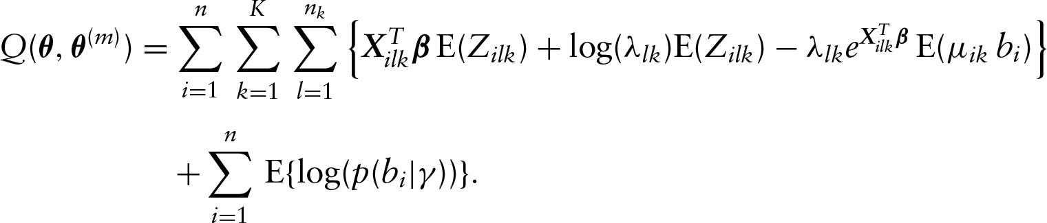
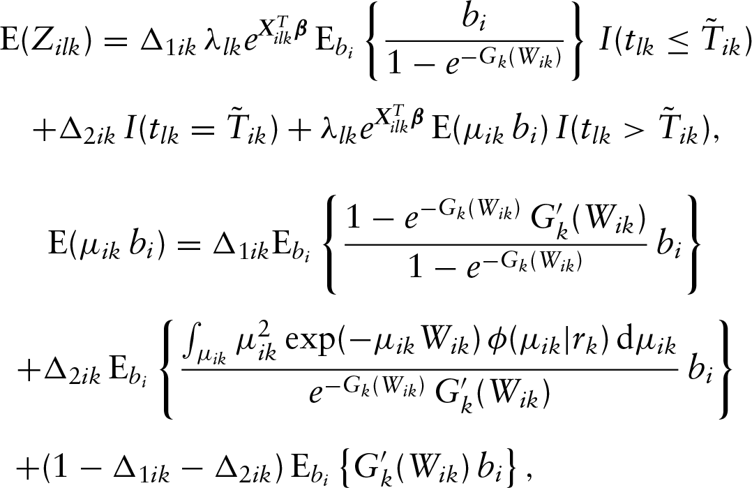
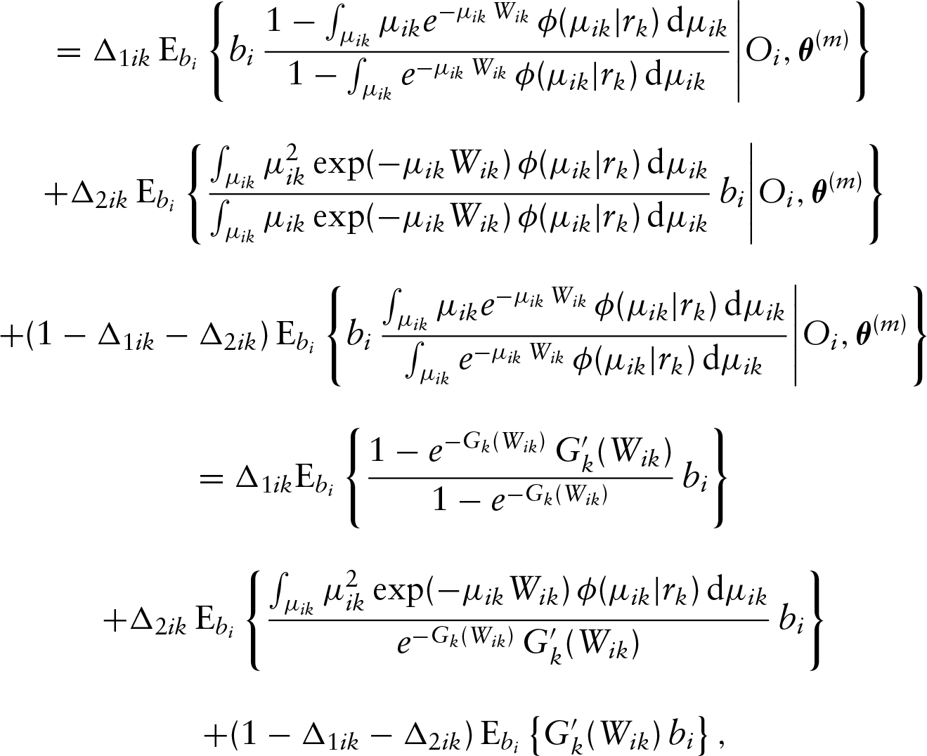
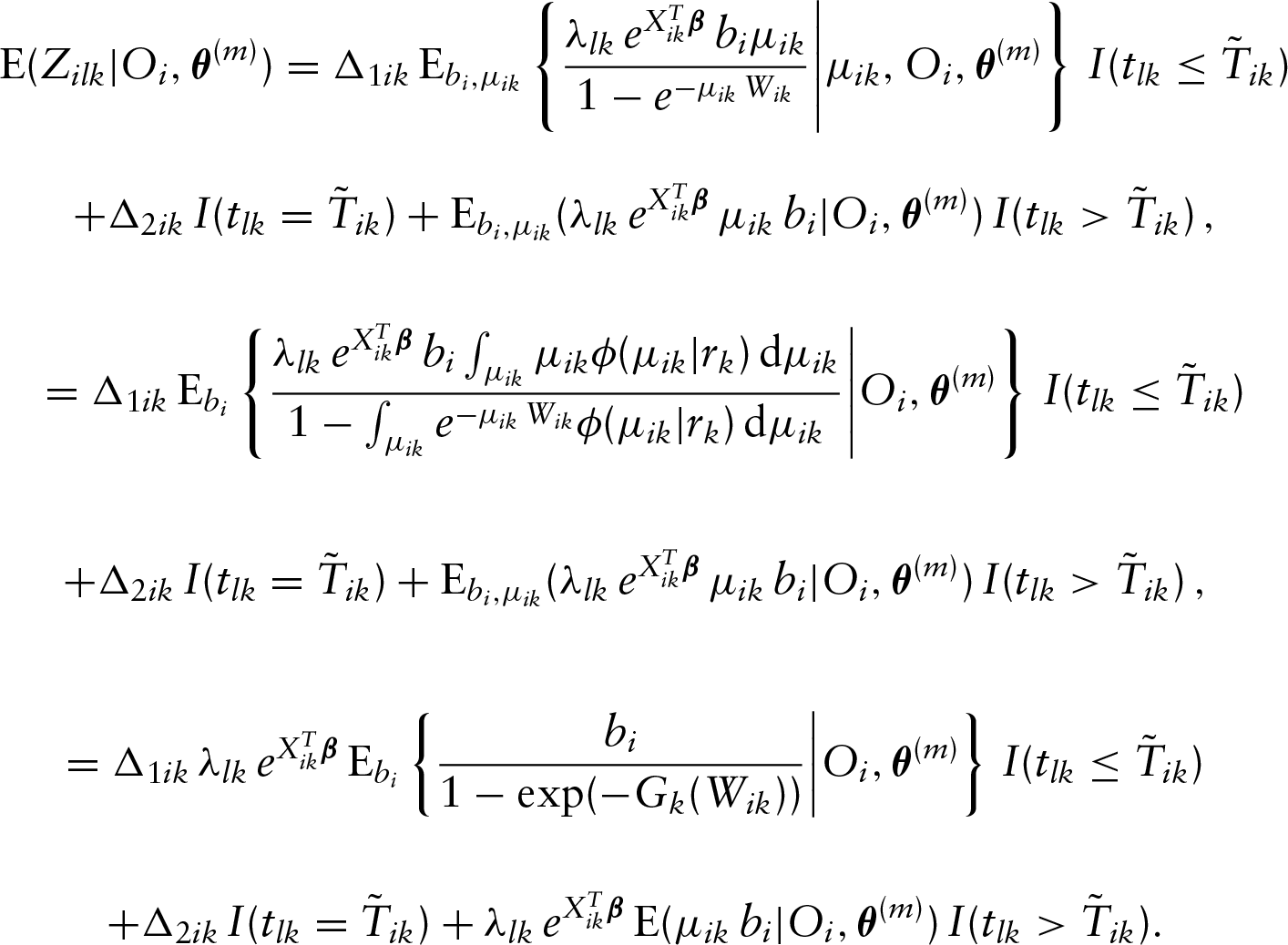
Now we are ready to present the E-step of the proposed algorithm. In this step, we need to determine the conditional expectations of all latent variables in the log-likelihood function $l_{c} (θ) = log L_{c} (θ)$ , which yields

\begin{matrix} Q (θ, θ^{(m)}) = \sum_{i = 1}^{n} \sum_{k = 1}^{K} \sum_{l = 1}^{n_{k}} \{X_{ilk}^{T} β E (Z_{ilk}) + log (λ_{lk}) E (Z_{ilk}) - λ_{lk} e^{X_{ilk}^{T} β} E (μ_{ik} b_{i})\} \\ + \sum_{i = 1}^{n} E {log (p (b_{i} | γ))} . \end{matrix}

Note that here, for notational simplicity, we have ignored the conditional arguments in all conditional expectations. In the above,

\begin{matrix} E (Z_{ilk}) = Δ_{1 ik} λ_{lk} e^{X_{ilk}^{T} β} E_{b_{i}} \{\frac{b_{i}}{1 - e^{- G_{k} (W_{ik})}}\} I (t_{lk} \leq {\tilde{T}}_{ik}) \\ + Δ_{2 ik} I (t_{lk} = {\tilde{T}}_{ik}) + λ_{lk} e^{X_{ilk}^{T} β} E (μ_{ik} b_{i}) I (t_{lk} > {\tilde{T}}_{ik}), \\ E (μ_{ik} b_{i}) = Δ_{1 ik} E_{b_{i}} \{\frac{1 - e^{- G_{k} (W_{ik})} G_{k}^{'} (W_{ik})}{1 - e^{- G_{k} (W_{ik})}} b_{i}\} \\ + Δ_{2 ik} E_{b_{i}} \{\frac{\int_{μ_{ik}} μ_{ik}^{2} exp (- μ_{ik} W_{ik}) ϕ (μ_{ik} | r_{k}) d μ_{ik}}{e^{- G_{k} (W_{ik})} G_{k}^{'} (W_{ik})} b_{i}\} \\ + (1 - Δ_{1 ik} - Δ_{2 ik}) E_{b_{i}} \{G_{k}^{'} (W_{ik}) b_{i}\}, \end{matrix}

and

E {h (b_{i})} = \frac{\int_{b_{i}} h (b_{i}) ψ_{i} (b_{i}) p (b_{i} | γ) d b_{i}}{\int_{b_{i}} ψ_{i} (b_{i}) p (b_{i} | γ) d b_{i}},

where $W_{ik} = \sum_{t_{lk} \leq {\tilde{T}}_{ik}} λ_{lk} e^{X_{ilk}^{T} β} b_{i}$ , and

\begin{matrix} ψ_{i} (b_{i}) = \prod_{k = 1}^{K} {\{1 - exp [- G_{k} (W_{ik})]\}}^{Δ_{1 ik}} {\{\prod_{l = 1}^{n_{k}} {(λ_{lk} e^{X_{ilk}^{T} β} b_{i})}^{I (t_{lk} = {\tilde{T}}_{ik})} G_{k}^{'} (W_{ik})\}}^{Δ_{2 ik}} \\ exp \{- (1 - Δ_{1 ik}) G_{k} (W_{ik})\} . \end{matrix}

The details for deriving the above conditional expectations are given in Appendix A. Note that if $ϕ (μ_{ik} | r_{k})$ is the density function of the gamma variable, one can calculate the following integration with respect to $μ_{ik}$ explicitly

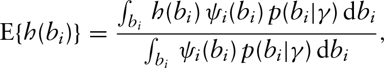
\int_{μ_{ik}} μ_{ik}^{2} exp (- μ_{ik} W_{ik}) ϕ (μ_{ik} | r_{k}) d μ_{ik} = (1 + r_{k}) (r_{k} W_{ik} + 1)^{- r_{k}^{- 1} - 2} .

Otherwise, we propose to employ Gauss–Laguerre quadrature technique to calculate the integrations with respect to $μ_{ik}$ that have no closed form.

For calculating $E {h (b_{i})}$ , in particular, we suggest to employ the probability integral transformation technique to transform $b_{i}$ into a standard normal variable and then adopt Gaussian–Hermite quadrature method to calculate this expectation. To illustrate this, let $ν_{i}$ be a standard normal random variable. Then we know that the distribution function of $ν_{i}$ , $Φ_{ν} (ν_{i})$ , follows the uniform distribution over $(0, 1)$ . Also note that $b_{i}$ follows a parametric distribution, and therefore, the cumulative distribution function of $b_{i}$ denoted by $Φ_{b} (b_{i})$ has specific form and also follows uniform distribution over $(0, 1)$ . This suggests that one can connect $b_{i}$ with a standard normal distributed variable $ν_{i}$ by setting $Φ_{b} (b_{i}) = Φ_{ν} (ν_{i})$ . Nelson et al. (2006) gave a detailed discussion about the probability integral transformation when the random effects or frailties follow a non-normal distribution. The numerical study below suggests that the joint use of the probability integral transformation and Gaussian–Hermite quadrature techniques provides a satisfactory performance in practice.

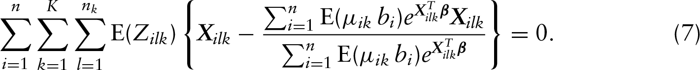
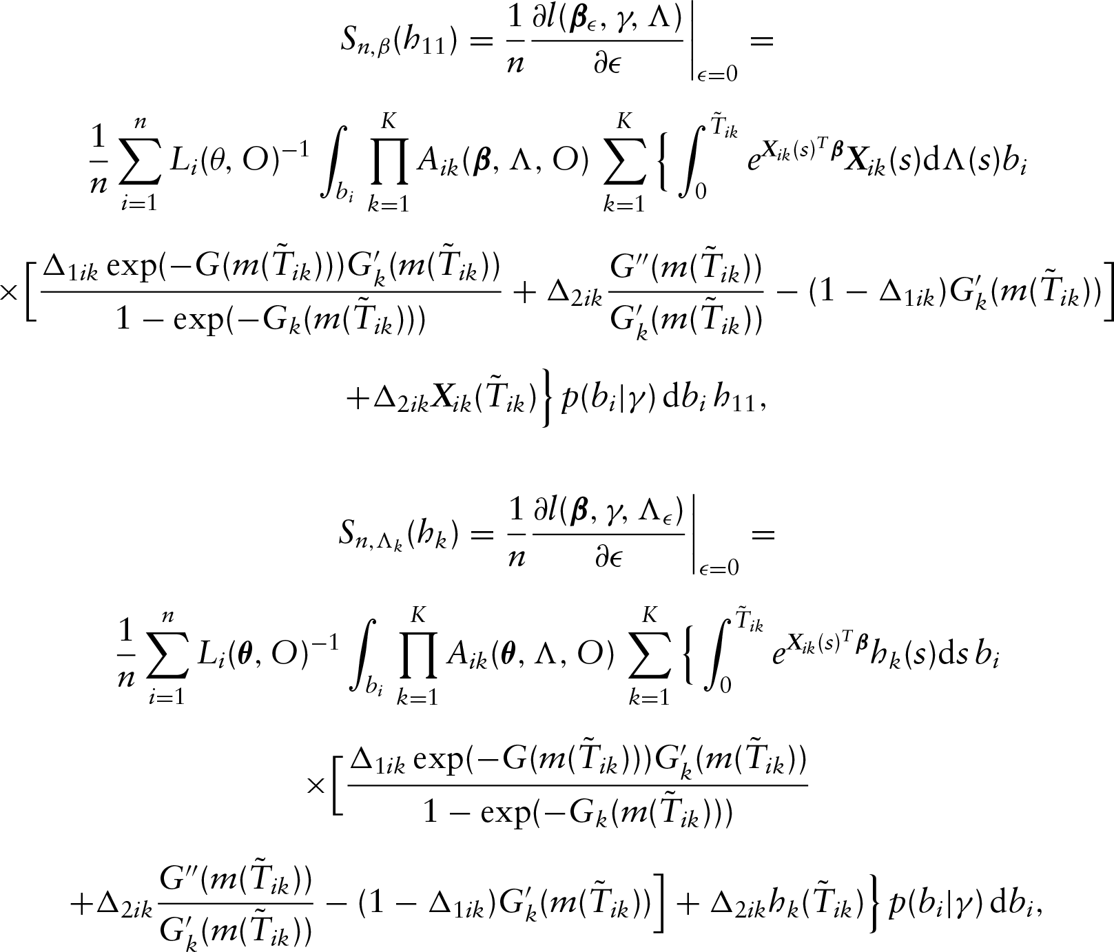
In the M-step of the EM algorithm, by setting $\partial Q (θ, θ^{(m)}) / \partial λ_{lk} = 0$ , we can update each $λ_{lk}$ as follows

λ_{lk} = \frac{\sum_{i = 1}^{n} E (Z_{ilk})}{\sum_{i = 1}^{n} E (μ_{ik} b_{i}) e^{X_{ilk}^{T} β}}, l = 1, \dots, n_{k}; k = 1, \dots, K .

(6)

Note that, for each $k$ , we have closed-form estimators for the $λ_{lk}$ ’s and this avoids the inversion of the possibly high-dimensional and ill-conditioned matrix in the optimization procedure. This is a desirable feature of the proposed method as it can be easily implemented. By plugging the estimators above into $Q (θ, θ^{(m)})$ , we have the estimation equation for the regression vector $β$ given as

\sum_{i = 1}^{n} \sum_{k = 1}^{K} \sum_{l = 1}^{n_{k}} E (Z_{ilk}) \{X_{ilk} - \frac{\sum_{i = 1}^{n} E (μ_{ik} b_{i}) e^{X_{ilk}^{T} β} X_{ilk}}{\sum_{i = 1}^{n} E (μ_{ik} b_{i}) e^{X_{ilk}^{T} β}}\} = 0 .

(7)

Finally, the estimator of $γ$ can be obtained by solving $\sum_{i = 1}^{n} \partial E {log (p (b_{i} | γ))} / \partial γ = 0$ .

In summary, by combining all steps described above, the proposed EM algorithm is as follows.

Step 0: Choose an initial estimator $θ^{(0)}$ .

Step 1: At the $(m + 1)$ th iteration, first calculate the conditional expectations $E (Z_{ilk})$ , $E (μ_{ik} b_{i})$ and $E {h (b_{i})}$ at $θ^{(m)}$ .

Step 2: Update $β^{(m + 1)}$ by solving the estimation equation $(7)$ with one-step Newton–Raphson method.

Step 3: $λ_{lk}^{(m + 1)}$ can be determined explicitly by $(6)$ , in which $β^{(m + 1)}$ is inserted.

Step 4: Calculate $γ^{(m + 1)}$ by solving $\sum_{i = 1}^{n} \partial E {log (p (b_{i} | γ))} / \partial γ = 0$ .

Step 5: Repeat Steps 1–4 until the convergence is achieved.

4 Asymptotic properties

Now we establish the asymptotic properties of the proposed estimators. Let $ζ = (β^{T}, γ)^{T}$ with $ζ_{0} = (β_{0}^{T}, γ_{0})^{T}$ and $θ_{0} = (ζ_{0}^{T}, Λ_{10}, . . ., Λ_{K 0})^{T}$ being the true values of $ζ$ and $θ$ , respectively. Also let ${\hat{θ}}_{n} = ({\hat{ζ}}_{n}^{T}, {\hat{Λ}}_{1 n}, . . ., {\hat{Λ}}_{Kn})^{T}$ denote the maximum likelihood estimator of $θ$ defined above. To establish the asymptotic properties of ${\hat{θ}}_{n}$ , we need the following regularity conditions.

(A1) $ζ_{0} = (β_{0}^{T}, γ_{0})^{T}$ belongs to a known compact set $A \times B$ in $R^{d + 1}$ . For each $k = 1, \dots, K$ , $Λ_{k 0} (\cdot)$ is continuously differentiable with positive derivatives in $[τ_{1}, τ_{2}]$ , where $[τ_{1}, τ_{2}]$ is the support of $\tilde{T}$ with $M^{- 1} < Λ_{k 0} (τ_{1}) < Λ_{k 0} (τ_{2}) < M$ and $M$ is a large positive constant.

(A2) For each $k$ , the vector $X_{k} (t)$ is uniformly bounded with finite total variation over $[τ_{1}, τ_{2}]$ and its left limit exists for any $t .$

(A3) If $h (t) + X_{k} (t)^{T} β = 0$ for all $t \in [τ_{1}, τ_{2}]$ with probability one, then $h (t) = 0$ for all $t \in [τ_{1}, τ_{2}]$ and $β = 0 .$

(A4) $G_{k}$ is twice continuously differentiable on $[0, \infty),$ with $G_{k} (0) = 0,$ $G_{k}^{'} (x) > 0$ and $G_{k} (\infty) = \infty .$ In addition, there exists a positive constant $ρ_{0}$ such that

lim sup_{x \to \infty} (1 + x)^{ρ_{0}} exp (- G_{k} (x)) < \infty .

(A5) For any smooth function $g (\cdot)$ , $sup_{γ \in B} \int_{b} g (b) p^{(j)} (b | γ) d b < \infty$ for $j = 0, 1, 2$ , where $p^{(j)} (b | γ)$ denotes the $j$ th derivative of $p (b | γ)$ with respect to $γ$ .

Conditions (A1) and (A2) are standard conditions in survival analysis (Zeng et al. 2016). Condition (A3) holds if the matrix $E ([1, X^{T} (t)]^{T} [1, X^{T} (t)])$ is nonsingular for all $t \in [τ_{1}, τ_{2}]$ . Condition (A4) holds for many transformation function families such as the logarithmic family $G (x) = r^{- 1} log (1 + r x) (r \geq 0)$ (Zeng et al. 2008). Condition (A5) is a commonly used assumption on the random-effect distribution for modelling the multivariate or clustered data with frailty models (Zeng et al. 2008).

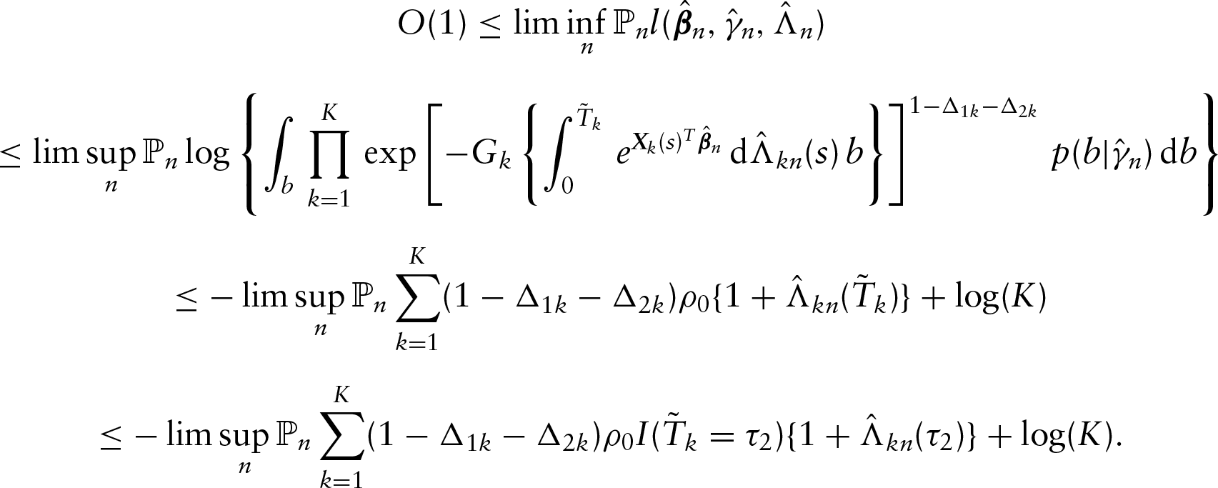
Theorem 1. Under regularity conditions (A1)–(A5) described above, $∥ {\hat{β}}_{n} - β_{0} ∥ \to 0$ , $∥ {\hat{γ}}_{n} - γ_{0} ∥ \to 0$ and $\sum_{k = 1}^{K} sup_{t \in [τ_{1}, τ_{2}]} | {\hat{Λ}}_{kn} (t) - Λ_{k 0} (t) | \to 0$ almost surely, where $∥ \cdot ∥$ is the Euclidean norm.

Theorem 2. Under regularity conditions (A1)–(A5) described above, the random element $\sqrt{n} ({\hat{β}}_{n} - β_{0}, {\hat{γ}}_{n} - γ_{0}, {\hat{Λ}}_{n} (\cdot) - Λ_{0} (\cdot))$ converges weakly to a zero-mean Gaussian process in the metric space $R^{(d + 1)} \times l^{\infty} [τ_{1}, τ_{2}]^{\otimes K},$ where $Λ = (Λ_{1}, \dots, Λ_{K})$ , $l^{\infty} [τ_{1}, τ_{2}]$ is a normed space consisting of all the bounded functions and the norm is defined as the supremum norm on $[τ_{1}, τ_{2}] .$ Furthermore, ${\hat{β}}_{n}$ and ${\hat{γ}}_{n}$ are asymptotically efficient.

The proofs of the two theorems above are deferred to the Appendix B. For inference about the parameters of interest, it is apparent that one needs to estimate the asymptotic covariance matrix of ${\hat{ζ}}_{n} = ({\hat{β}}_{n}^{T}, {\hat{γ}}_{n})^{T}$ . For this, it would be very difficult to derive the consistent estimator as discussed below and thus instead, we propose to employ the nonparametric bootstrap procedure (Su and Wang 2016). To be specific, we first repeatedly draw new datasets of sample size $n$ with replacement from the original observed data $O = (O_{i} = (O_{i 1}, . . ., O_{iK}); i = 1, \dots, n)$ for $Q$ times, where $Q$ is a prespecified positive integer. The newly resampled datasets are denoted by $O^{(q)}$ for $q = 1, \dots, Q$ . Let ${\hat{ζ}}_{n}^{(q)}$ denote the resulting estimator of $ζ$ based on $O^{(q)}$ . Then one can estimate the covariance matrix of ${\hat{ζ}}_{n}$ by the empirical covariance matrix of ${\hat{ζ}}_{n}^{(1)}, \dots, {\hat{ζ}}_{n}^{(Q)}$ .

5 A simulation study

A simulation study was conducted to assess the numerical performance of the proposed methodology in finite samples. In the study, the $T_{i}$ ’s were generated from the class of transformation models (1) with $G_{k} (x) = \log (1 + r_{k} x) / r_{k} (r_{k} \geq 0)$ and $Λ_{k} (t) = 0.2 t$ for $k = 1, 2$ . Here, we took each $r_{k}$ be 0, 0.5 or 1 and considered the combinations of different values of $r_{1}$ and $r_{2}$ . More details are given in the first two columns of the tables below. Note that the choices of $r_{k} = 0$ and $r_{k} = 1$ correspond to the proportional hazards and proportional odds frailty models, respectively. Here, we considered two frailty distributions: the log-normal frailty with mean one and variance $γ^{2}$ and the gamma frailty with mean one and variance $γ$ . For subject $i$ , we randomly generated the left-censored variable $L_{i}$ and the right-censored variable $R_{i}$ according to the uniform distributions $U (0, 1)$ and $U (3, 5),$ respectively. For the generation of covariates, we considered the two-dimensional coavariate setting with $X_{ik 1}$ ’s following the Bernoulli distribution with the success probability of 0.5 and $X_{ik 2}$ ’s being generated from $U (0, 1) .$ The true values of $(β_{1}, β_{2}, γ)$ denoted by $(β_{10}, β_{20}, γ_{0})$ were set to be $(0.5, - 0.5, 1)$ . The results below are based on 500 replications, $Q = 100$ and $n = 200$ or $400$ .

Table 1:
Simulation results for the log-normal frailty

$n = 200$ $n = 400$

$r_{1}$ $r_{2}$ Bias SSE SEE CP Bias SSE SEE CP

0 0 $β_{1} = 0.5$ $-$ 0.016 0.219 0.215 94.0 $-$ 0.001 0.156 0.155 95.7

$β_{2} = - 0.5$ 0.030 0.369 0.372 94.3 0.001 0.265 0.266 94.7

$γ = 1$ $-$ 0.023 0.151 0.155 94.7 0.019 0.122 0.111 95.3

0.5 0.5 $β_{1} = 0.5$ $-$ 0.014 0.242 0.243 94.0 $-$ 0.003 0.164 0.170 94.7

$β_{2} = - 0.5$ $-$ 0.014 0.439 0.418 93.5 $-$ 0.006 0.273 0.295 94.7

$γ = 1$ $-$ 0.025 0.196 0.190 95.6 $-$ 0.004 0.138 0.134 95.3

0.5 1 $β_{1} = 0.5$ $-$ 0.007 0.262 0.250 93.8 0.002 0.186 0.176 95.0

$β_{2} = - 0.5$ 0.028 0.458 0.438 94.0 0.011 0.295 0.305 94.8

$γ = 1$ $-$ 0.020 0.213 0.206 94.6 $-$ 0.013 0.139 0.139 94.6

1 1 $β_{1} = 0.5$ 0.024 0.253 0.262 95.3 $-$ 0.005 0.195 0.188 94.6

$β_{2} = - 0.5$ 0.028 0.468 0.455 94.7 0.003 0.334 0.317 94.4

$γ = 1$ $-$ 0.022 0.232 0.217 94.0 $-$ 0.019 0.145 0.151 94.0

			$n = 200$		$n = 400$
0	0	$β_{1} = 0.5$	$-$ 0.016	0.219	0.215	94.0	$-$ 0.001	0.156	0.155	95.7
		$β_{2} = - 0.5$	0.030	0.369	0.372	94.3	0.001	0.265	0.266	94.7
		$γ = 1$	$-$ 0.023	0.151	0.155	94.7	0.019	0.122	0.111	95.3
0.5	0.5	$β_{1} = 0.5$	$-$ 0.014	0.242	0.243	94.0	$-$ 0.003	0.164	0.170	94.7
		$β_{2} = - 0.5$	$-$ 0.014	0.439	0.418	93.5	$-$ 0.006	0.273	0.295	94.7
		$γ = 1$	$-$ 0.025	0.196	0.190	95.6	$-$ 0.004	0.138	0.134	95.3
0.5	1	$β_{1} = 0.5$	$-$ 0.007	0.262	0.250	93.8	0.002	0.186	0.176	95.0
		$β_{2} = - 0.5$	0.028	0.458	0.438	94.0	0.011	0.295	0.305	94.8
		$γ = 1$	$-$ 0.020	0.213	0.206	94.6	$-$ 0.013	0.139	0.139	94.6
1	1	$β_{1} = 0.5$	0.024	0.253	0.262	95.3	$-$ 0.005	0.195	0.188	94.6
		$β_{2} = - 0.5$	0.028	0.468	0.455	94.7	0.003	0.334	0.317	94.4
		$γ = 1$	$-$ 0.022	0.232	0.217	94.0	$-$ 0.019	0.145	0.151	94.0

Table 2:

Simulation results for the gamma frailty

			$n = 200$				$n = 400$
$r_{1}$	$r_{2}$		Bias	SSE	SEE	CP	Bias	SSE	SEE	CP
0	0	$β_{1} = 0.5$	$-$ 0.017	0.227	0.218	94.7	$-$ 0.007	0.142	0.152	94.7
		$β_{2} = - 0.5$	0.011	0.361	0.383	96.0	$-$ 0.008	0.278	0.263	94.7
		$γ = 1$	$-$ 0.052	0.270	0.275	96.0	$-$ 0.030	0.197	0.197	95.0
0.5	0.5	$β_{1} = 0.5$	$-$ 0.020	0.251	0.243	95.0	0.002	0.182	0.173	96.0
		$β_{2} = - 0.5$	$-$ 0.007	0.425	0.421	94.3	0.004	0.281	0.297	95.3
		$γ = 1$	$-$ 0.061	0.338	0.323	97.0	$-$ 0.022	0.281	0.286	95.7
0.5	1	$β_{1} = 0.5$	$-$ 0.022	0.257	0.251	94.7	0.011	0.171	0.178	96.0
		$β_{2} = - 0.5$	0.031	0.452	0.437	95.0	$-$ 0.007	0.308	0.308	94.7
		$γ = 1$	$-$ 0.056	0.353	0.342	95.3	$-$ 0.052	0.264	0.262	96.3
1	1	$β_{1} = 0.5$	$-$ 0.026	0.249	0.263	96.3	$-$ 0.004	0.183	0.187	94.3
		$β_{2} = - 0.5$	0.025	0.456	0.456	94.0	$-$ 0.009	0.335	0.321	95.0
		$γ = 1$	$-$ 0.082	0.400	0.353	96.3	$-$ 0.072	0.302	0.272	95.7

The results under the log-normal and gamma frailties are given in Tables 1 and 2, respectively. We mainly focused on the estimated bias (Bias) given by the average of the estimates minus the true value, the sample standard error (SSE) of the obtained estimates, the average of the standard error estimates (SEE), and the 95% empirical coverage probability (CP). One can see from both tables that the proposed nonparametric maximum likelihood estimates have little biases and the SEE based on nonparametric bootstrap method are in well agreement with the simulated SSE. Also, all empirical CPs are quite close to the nominal value, indicating that the normal distribution provides a reasonable approximation to the distribution of the proposed estimator.

Note that in the proposed method, we have assumed that the distribution for the

b_{i}

’s is known and thus it is of interest to investigate how sensitive the proposed method is to the misspecification of the frailty distribution. For this, we generated the latent variables

b_{i}

’s from the gamma distribution with mean one and variance one, but fitted the simulated data with the transformation models with the log-normal frailty, and kept the other model specifications being the same as above. The results given in Table 3 indicate that the proposed method seems to work well for the situations considered here.

Table 3:

Simulation results under the misspecified frailty distribution

			$n = 200$				$n = 400$
$r_{1}$	$r_{2}$		Bias	SSE	SEE	CP	Bias	SSE	SEE	CP
0	0	$β_{1} = 0.5$	$-$ 0.020	0.199	0.196	93.6	$-$ 0.017	0.149	0.140	95.0
		$β_{2} = - 0.5$	0.023	0.343	0.334	94.4	$-$ 0.007	0.255	0.242	94.6
0.5	0.5	$β_{1} = 0.5$	0.021	0.218	0.222	95.8	$-$ 0.019	0.154	0.156	95.0
		$β_{2} = - 0.5$	$-$ 0.031	0.395	0.388	93.8	0.018	0.267	0.271	94.4
0.5	1	$β_{1} = 0.5$	$-$ 0.014	0.212	0.220	94.8	$-$ 0.010	0.160	0.164	95.0
		$β_{2} = - 0.5$	0.019	0.370	0.401	95.8	0.004	0.283	0.284	95.2
1	1	$β_{1} = 0.5$	$-$ 0.014	0.251	0.259	94.0	$-$ 0.010	0.187	0.182	95.7
		$β_{2} = - 0.5$	0.037	0.462	0.451	96.3	0.014	0.318	0.317	96.3

6 An application

In this section, we apply the proposed methodology to a set of real doubly censored data arising form the AIDS Clinical Trials Group Protocol 320 (ACTG 320) study conducted between 29 January 1996 and 27 January 1997 (Hammer et al. (1997); Cai et al. 2014). The aim of this study was to compare the treatment effects of the 2-drug combination of zidovudine (ZDV) and lamivudine (3TC) and the 3-drug combination of ZDV, 3TC and indinavir (RTV) for the type-I HIV infected patients. In AIDS studies, two indicators are commonly used for assessing the good curative effect of a treatment. One is the increment of the cluster of differentiation 4 (CD4) count and the other is the decrement of the plasma HIV-1 RNA level. The measurement of the RNA level is usually done by the NucliSens assay, which is known to be highly unreliable if the RNA level is below 400 or above 750 000 per millilitre of plasma. In other words, the RNA level suffers left censoring at 400 and right censoring at 750 000. Therefore, we can only have doubly censored data on the plasma HIV-1 RNA level under this situation.

For the analysis here, we will consider the 838 patients who were followed up to 24 weeks with the focus on the changes in CD4 count and RNA level between their values at week 0 and week 24. For this, define $T_{i 1}$ to be the CD4 value at week 24 minus its value at week 0 and $T_{i 2}$ the ${log}_{10}$ RNA level at week 0 denoted by $l_{0}$ minus its level at week 24. Note that here we used different definitions for the two indicators because of their nature and relationship with the AIDS progress. For this set of data, the measurements of the RNA at week 0 for all subjects are within the limit of quantification, and therefore, $T_{i 2}$ can be either left censored by $l_{0} - 5.88$ or right censored by $l_{0} - 2.60$ . The percentages of the left-censored and right-censored observation for the RNA level are 1.67% and 29.12%, respectively. Also note that here we do not have any censoring on $T_{i 1}$ , which corresponds to the situation where $Δ_{1 ik} = 0$ and $Δ_{2 ik} = 1$ for $k = 1$ and $i = 1, \dots, n$ . In the following, we define the covariate $trt$ be $1$ if the patient was in the 3-drug combination group and 0 otherwise.

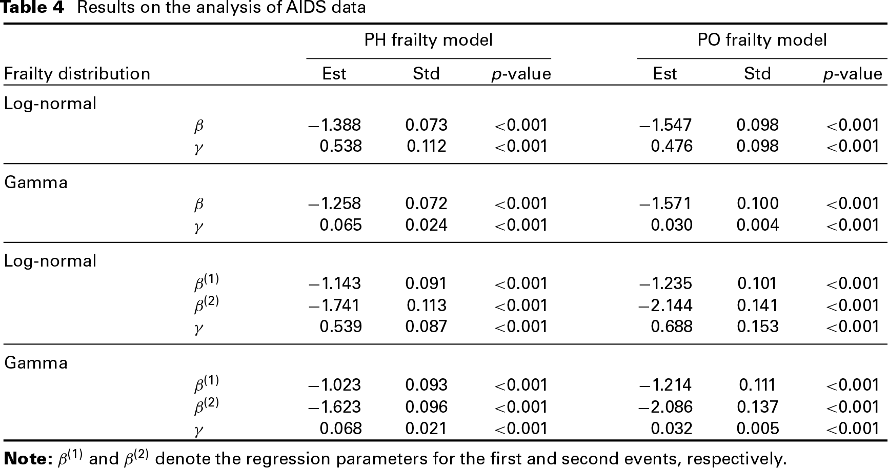
To fit the class of the models (1), as in the simulation study, we considered both the log-normal and gamma frailties and set $G_{k} (x) = \log (1 + r_{k} x) / r_{k} (r_{k} \geq 0)$ , the logarithmic transformation function. We first assumed that the covariate had the same effect on the two events, and then performed the analysis by assuming that the effects may be different, which can be easily achieved by redefining a larger covariate vector in the proposed models. Here, we considered each $r_{k}$ ranging from 0 to 3 with an increment of 0.1 and performed grid search for the optimal $r_{1}$ and $r_{2}$ by considering all different combinations. Through the analysis, it turned out that the optimal model was given by proportional hazards model (PH frailty model) with gamma frailty and different covariate effects, which yields the largest log-likelihood value.

The results are summarized in Tables 4 and 5, and we also report the results obtained from the commonly used proportional odds frailty model (PO frailty model) for comparison. One can see from the two tables above that all results consistently indicate that the treatment effect was significant. Note that the negative estimate of the regression parameter corresponds to a lower hazard value or higher survival value. This indicates that the plasma HIV-1 RNA level decreased more and the CD4 count increased more compared to the baseline values, respectively. In other words, the 3-drug combination was significantly more effective in reducing the plasma HIV-1 RNA level and increasing the CD4 count than the 2-drug combination. This also suggests the beneficial effect of the addition of RTV for treating the AIDS infected patients. Additionally, the frailty variance is significant under 0.05 level, which indicates that there exists the positive correlation between the two outcomes.

7 Discussion and concluding remarks

In this article, we discussed regression analysis of multivariate doubly censored data with a wide class of semiparametric transformation frailty models. For inference, a novel and computationally stable EM algorithm was developed with the use of some Poisson variables to determine the proposed nonparametric maximum likelihood estimators. The resulting estimators of the finite-dimensional parameters were shown to be consistent, asymptotically normal and semiparametrically efficient. Also the numerical results obtained by a simulation study indicated that the proposed method works well in finite samples.

The presence of the left-censorship in doubly censored data poses great computational challenges in deriving the nonparametric maximum likelihood estimators for the semiparametric regression models. This is mainly due to the complex form of the observed data likelihood function and the lack of the closed-form solutions for the high-dimensional parameters involved in the cumulative hazard function. However, the proposed usage of some Poisson variables in the data augmentation part allows us to calculate the high-dimensional parameters $λ_{lk}$ ’s with closed forms and the finite-dimensional parameters $β$ and $γ$ can be updated with one-step Newton–Raphson approach separately. This avoids the inversion of the possibly high-dimensional and ill-conditioned matrix, and thus makes the estimating procedure easily implemented. Furthermore, the joint usage of the probability integral transformation technique and Gauss–Hermite quadrature method can calculate the conditional expectations in the E-step under various frailty distributions. Thus, the proposed method can apply to more general situations in practice.

Table 4:
Results on the analysis of AIDS data

PH frailty model PO frailty model

Frailty distribution $Est$ $Std$ $p$ -value $Est$ $Std$ $p$ -value

Log-normal

$β$ $-$ 1.388 0.073 $<$ 0.001 $-$ 1.547 0.098 $<$ 0.001

$γ$ 0.538 0.112 $<$ 0.001 0.476 0.098 $<$ 0.001

Gamma

$β$ $-$ 1.258 0.072 $<$ 0.001 $-$ 1.571 0.100 $<$ 0.001

$γ$ 0.065 0.024 $<$ 0.001 0.030 0.004 $<$ 0.001

Log-normal

$β^{(1)}$ $-$ 1.143 0.091 $<$ 0.001 $-$ 1.235 0.101 $<$ 0.001

$β^{(2)}$ $-$ 1.741 0.113 $<$ 0.001 $-$ 2.144 0.141 $<$ 0.001

$γ$ 0.539 0.087 $<$ 0.001 0.688 0.153 $<$ 0.001

Gamma

$β^{(1)}$ $-$ 1.023 0.093 $<$ 0.001 $-$ 1.214 0.111 $<$ 0.001

$β^{(2)}$ $-$ 1.623 0.096 $<$ 0.001 $-$ 2.086 0.137 $<$ 0.001

$γ$ 0.068 0.021 $<$ 0.001 0.032 0.005 $<$ 0.001

		PH frailty model		PO frailty model
Frailty distribution		$Est$	$Std$	$p$ -value	$Est$	$Std$	$p$ -value
Log-normal
	$β$	$-$ 1.388	0.073	$<$ 0.001	$-$ 1.547	0.098	$<$ 0.001
	$γ$	0.538	0.112	$<$ 0.001	0.476	0.098	$<$ 0.001
Gamma
	$β$	$-$ 1.258	0.072	$<$ 0.001	$-$ 1.571	0.100	$<$ 0.001
	$γ$	0.065	0.024	$<$ 0.001	0.030	0.004	$<$ 0.001
Log-normal
	$β^{(1)}$	$-$ 1.143	0.091	$<$ 0.001	$-$ 1.235	0.101	$<$ 0.001
	$β^{(2)}$	$-$ 1.741	0.113	$<$ 0.001	$-$ 2.144	0.141	$<$ 0.001
	$γ$	0.539	0.087	$<$ 0.001	0.688	0.153	$<$ 0.001
Gamma
	$β^{(1)}$	$-$ 1.023	0.093	$<$ 0.001	$-$ 1.214	0.111	$<$ 0.001
	$β^{(2)}$	$-$ 1.623	0.096	$<$ 0.001	$-$ 2.086	0.137	$<$ 0.001
	$γ$	0.068	0.021	$<$ 0.001	0.032	0.005	$<$ 0.001

Note: $β^{(1)}$ and $β^{(2)}$ denote the regression parameters for the first and second events, respectively.

Note that in the preceding sections, we showed that the proposed method can deal with the type of data in which the outcome variable may not a typical failure time. For such outcomes, a natural or straightforward approach may be linear model-based procedures if there is no censoring. However, in the presence of double censoring, the development of some estimation procedures may not be an easy task, and instead, the hazard-based method can provide a good alternative. Among others, Cai and Cheng (2004) and Li et al. (2018) discussed such approaches for the analysis of doubly censored data.

In many scientific studies, one often assumes that all subjects under study will eventually experience the event of interest if the follow-up is sufficient long. However, in practice, there may exist a non-susceptible subpopulation, which is usually referred to as cured fraction and in this situation, some cure models may provide a better fit. Hence, it may be helpful to extend the proposed method to this cured situation. It is also necessary to allow for informative censoring in the analysis where the outcome variable of interest and the censoring variables are not independent as often happen in many medical research fields (Li et al. 2017). Another direction for future research is to develop the estimation procedure for other commonly used semiparamteric regression models such as the additive hazards model (Lin and Ying 1994).

8 Appendix

Appendix A: More details about the proposed EM algorithm

Note that we have re-expressed likelihood function (4) with the equivalent form (5) by using some Poisson variables, and to see this derivation, we note that if $Δ_{1 ik} = 1$ ,

\begin{matrix} \Pr (\sum_{t_{lk} \leq {\tilde{T}}_{ik}} Z_{ilk} > 0) = 1 - \Pr (\sum_{t_{lk} \leq {\tilde{T}}_{ik}} Z_{ilk} = 0) = 1 - \prod_{t_{lk} \leq {\tilde{T}}_{ik}} exp [- λ_{lk} e^{X_{ilk}^{T} β} μ_{ik} b_{i}], \\ = 1 - exp [- μ_{ik} (\sum_{t_{lk} \leq {\tilde{T}}_{ik}} λ_{lk} e^{X_{ilk}^{T} β} b_{i})], \end{matrix}

if $Δ_{2 ik} = 1$ , we have

\begin{matrix} \Pr (\sum_{t_{lk} < {\tilde{T}}_{ik}} Z_{ilk} = 0) \Pr (Z_{ilk} |_{t_{lk} = {\tilde{T}}_{ik}} = 1) \\ = \prod_{t_{lk} < {\tilde{T}}_{ik}} exp [- λ_{lk} e^{X_{ilk}^{T} β} μ_{ik} b_{i}] \prod_{l = 1}^{n_{k}} {(λ_{lk} e^{X_{ilk}^{T} β} μ_{ik} b_{i})}^{I (t_{lk} = {\tilde{T}}_{ik})} \\ = \prod_{l = 1}^{n_{k}} {(λ_{lk} e^{X_{ilk}^{T} β} μ_{ik} b_{i})}^{I (t_{lk} = {\tilde{T}}_{ik})} exp [- μ_{ik} (\sum_{t_{lk} < {\tilde{T}}_{ik}} λ_{lk} e^{X_{ilk}^{T} β} b_{i})] \end{matrix}

and if $Δ_{1 ik} = Δ_{2 ik} = 0$ , we have

\begin{matrix} \Pr (\sum_{t_{lk} \leq {\tilde{T}}_{ik}} Z_{ilk} = 0) = \prod_{t_{lk} \leq {\tilde{T}}_{ik}} exp [- λ_{lk} e^{X_{ilk}^{T} β} μ_{ik} b_{i}] \\ = exp [- μ_{ik} (\sum_{t_{lk} \leq {\tilde{T}}_{ik}} λ_{lk} e^{X_{ilk}^{T} β} b_{i})] . \end{matrix}

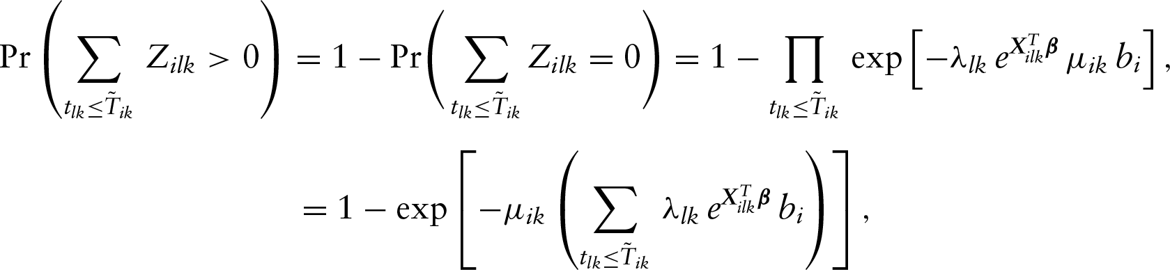
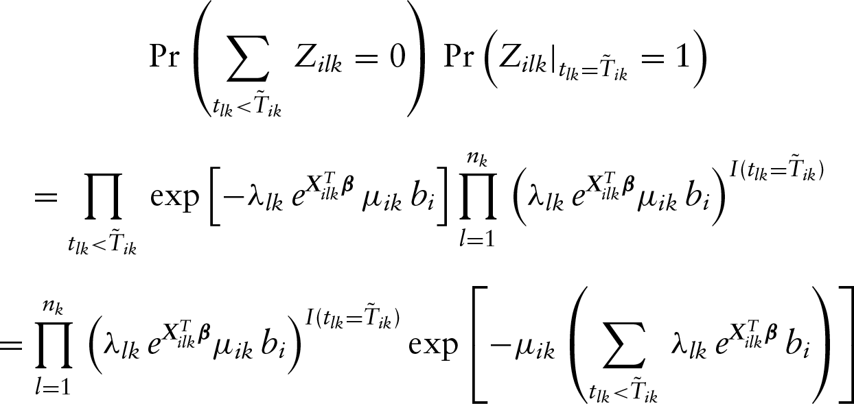
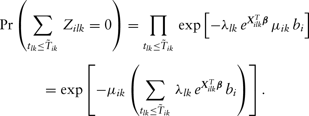
In the following, we will discuss the derivation of the conditional expectations $E (μ_{ik} b_{i})$ and $E (Z_{ilk})$ in the E-step. Here, we denote the observed data for subject $i$ by $O_{i} = (O_{i 1}, \dots, O_{iK})$ and current estimates of parameters by $θ^{(m)}$ in all conditional expectations. Also the following derivations of the following conditional expectations are based on the constraints in the complete likelihood function, $\sum_{t_{lk} \leq {\tilde{T}}_{ik}} Z_{ilk} > 0$ if $Δ_{1 ik} = 1$ , $\sum_{t_{lk} < {\tilde{T}}_{ik}} Z_{ilk} = 0$ and $Z_{ilk} |_{t_{lk} = {\tilde{T}}_{ik}} = 1$ if $Δ_{2 ik} = 1$ and $\sum_{t_{lk} \leq {\tilde{T}}_{ik}} Z_{ilk} = 0$ if $Δ_{1 ik} + Δ_{2 ik} = 0$ . Let $W_{ik} = \sum_{t_{lk} \leq {\tilde{T}}_{ik}} λ_{lk} e^{X_{ilk}^{T} β} b_{i}$ , by using the law of iterated expectations and Bayes’ theorem, we know that $E (μ_{ik} b_{i} | O_{i}, θ^{(m)}) = E_{b_{i}} \{b_{i} E (μ_{ik} | O_{i}, θ^{(m)}) | O_{i}, θ^{(m)}\}$

\begin{matrix} = Δ_{1 ik} E_{b_{i}} \{b_{i} \frac{1 - \int_{μ_{ik}} μ_{ik} e^{- μ_{ik} W_{ik}} ϕ (μ_{ik} | r_{k}) d μ_{ik}}{1 - \int_{μ_{ik}} e^{- μ_{ik} W_{ik}} ϕ (μ_{ik} | r_{k}) d μ_{ik}} | O_{i}, θ^{(m)}\} \\ + Δ_{2 ik} E_{b_{i}} \{\frac{\int_{μ_{ik}} μ_{ik}^{2} exp (- μ_{ik} W_{ik}) ϕ (μ_{ik} | r_{k}) d μ_{ik}}{\int_{μ_{ik}} μ_{ik} exp (- μ_{ik} W_{ik}) ϕ (μ_{ik} | r_{k}) d μ_{ik}} b_{i} | O_{i}, θ^{(m)}\} \\ + (1 - Δ_{1 ik} - Δ_{2 ik}) E_{b_{i}} \{b_{i} \frac{\int_{μ_{ik}} μ_{ik} e^{- μ_{ik} W_{ik}} ϕ (μ_{ik} | r_{k}) d μ_{ik}}{\int_{μ_{ik}} e^{- μ_{ik} W_{ik}} ϕ (μ_{ik} | r_{k}) d μ_{ik}} | O_{i}, θ^{(m)}\} \\ = Δ_{1 ik} E_{b_{i}} \{\frac{1 - e^{- G_{k} (W_{ik})} G_{k}^{'} (W_{ik})}{1 - e^{- G_{k} (W_{ik})}} b_{i}\} \\ + Δ_{2 ik} E_{b_{i}} \{\frac{\int_{μ_{ik}} μ_{ik}^{2} exp (- μ_{ik} W_{ik}) ϕ (μ_{ik} | r_{k}) d μ_{ik}}{e^{- G_{k} (W_{ik})} G_{k}^{'} (W_{ik})} b_{i}\} \\ + (1 - Δ_{1 ik} - Δ_{2 ik}) E_{b_{i}} \{G_{k}^{'} (W_{ik}) b_{i}\}, \end{matrix}

and

\begin{matrix} E (Z_{ilk} | O_{i}, θ^{(m)}) = Δ_{1 ik} E_{b_{i}, μ_{ik}} \{\frac{λ_{lk} e^{X_{ik}^{T} β} b_{i} μ_{ik}}{1 - e^{- μ_{ik} W_{ik}}} | μ_{ik}, O_{i}, θ^{(m)}\} I (t_{lk} \leq {\tilde{T}}_{ik}) \\ + Δ_{2 ik} I (t_{lk} = {\tilde{T}}_{ik}) + E_{b_{i}, μ_{ik}} (λ_{lk} e^{X_{ik}^{T} β} μ_{ik} b_{i} | O_{i}, θ^{(m)}) I (t_{lk} > {\tilde{T}}_{ik}), \\ = Δ_{1 ik} E_{b_{i}} \{\frac{λ_{lk} e^{X_{ik}^{T} β} b_{i} \int_{μ_{ik}} μ_{ik} ϕ (μ_{ik} | r_{k}) d μ_{ik}}{1 - \int_{μ_{ik}} e^{- μ_{ik} W_{ik}} ϕ (μ_{ik} | r_{k}) d μ_{ik}} | O_{i}, θ^{(m)}\} I (t_{lk} \leq {\tilde{T}}_{ik}) \\ + Δ_{2 ik} I (t_{lk} = {\tilde{T}}_{ik}) + E_{b_{i}, μ_{ik}} (λ_{lk} e^{X_{ik}^{T} β} μ_{ik} b_{i} | O_{i}, θ^{(m)}) I (t_{lk} > {\tilde{T}}_{ik}), \\ = Δ_{1 ik} λ_{lk} e^{X_{ik}^{T} β} E_{b_{i}} \{\frac{b_{i}}{1 - exp (- G_{k} (W_{ik}))} | O_{i}, θ^{(m)}\} I (t_{lk} \leq {\tilde{T}}_{ik}) \\ + Δ_{2 ik} I (t_{lk} = {\tilde{T}}_{ik}) + λ_{lk} e^{X_{ik}^{T} β} E (μ_{ik} b_{i} | O_{i}, θ^{(m)}) I (t_{lk} > {\tilde{T}}_{ik}) . \end{matrix}

Appendix B: Proofs of Theorems 1 and 2

For the proofs, we will mainly use some results about empirical processes given in (van der Vaart and Wellner 1996). In the following, for a function $f$ and a random variable $X$ with the distribution $F$ , define $ℙ f = \int f (x) d F (x)$ and $ℙ_{n} f = n^{- 1} \sum_{i = 1}^{n} f (X_{i})$ . Let $∥ \cdot ∥$ denote the Euclidean norm and $∥ \cdot ∥_{2}$ denote the usual $L_{2}$ norm.

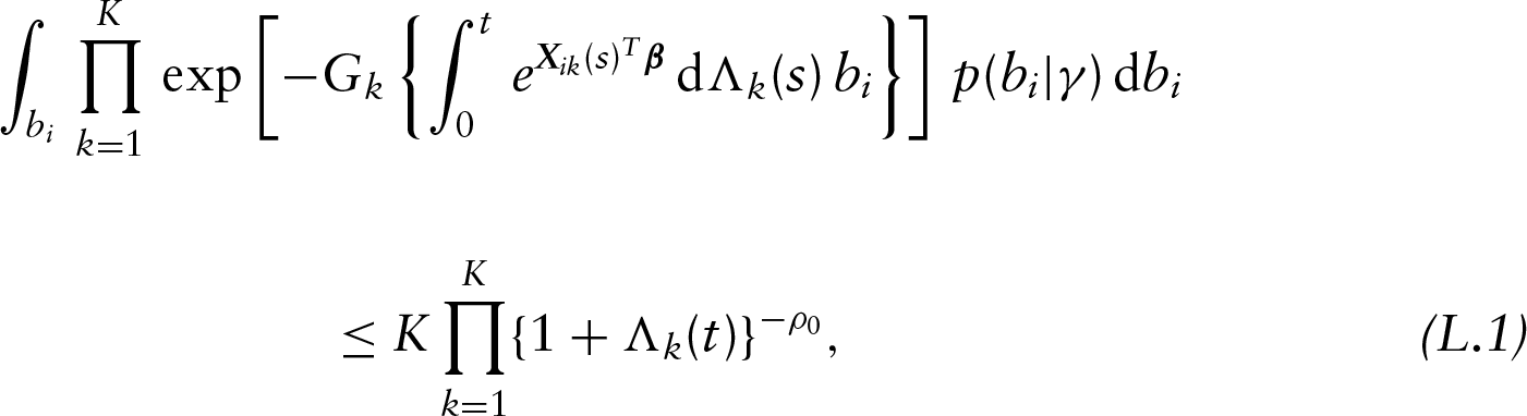
Lemma 1. Under conditions (A4) and (A5), with probability one, we have

\begin{matrix} \int_{b_{i}} \prod_{k = 1}^{K} \exp [- G_{k} {\int_{0}^{t} e^{X_{i k} {(s)}^{T} β} d Λ_{k} (s) b_{i}}] p (b_{i} | γ) d b_{i} \\ \leq K \prod_{k = 1}^{K} {1 + Λ_{k} (t)}^{- ρ_{0}}, \end{matrix}

(L.1)

where $K$ represents a generic constant that may vary from place to place and is independent of $β, γ$ and $Λ$ .

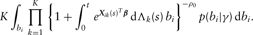
Proof. Under condition (A4), we have $exp (- G (x)) < K (1 + x)^{- ρ_{0}}$ . Therefore, the left-hand side of equation (L.1) is bounded by

K \int_{b_{i}} \prod_{k = 1}^{K} {\{1 + \int_{0}^{t} e^{X_{ik} (s)^{T} β} d Λ_{k} (s) b_{i}\}}^{- ρ_{0}} p (b_{i} | γ) d b_{i} .

Let $M_{1}$ be a large positive constant such that $M_{1}^{- 1} \leq e^{X_{ik} (t)^{T} β} \leq M_{1}$ . We can show that

1 + \int_{0}^{t} e^{X_{ik} (s)^{T} β} d Λ_{k} (s) b_{i} \geq 1 + M_{1}^{- 1} Λ_{k} (t) b_{i} \geq M_{1}^{- 1} b_{i} (1 + Λ_{k} (t)) .

Therefore,

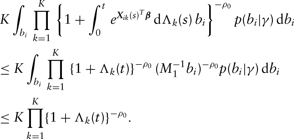
\begin{matrix} K \int_{b_{i}} \prod_{k = 1}^{K} {\{1 + \int_{0}^{t} e^{X_{ik} (s)^{T} β} d Λ_{k} (s) b_{i}\}}^{- ρ_{0}} p (b_{i} | γ) d b_{i} \\ \leq K \int_{b_{i}} \prod_{k = 1}^{K} {\{1 + Λ_{k} (t)\}}^{- ρ_{0}} (M_{1}^{- 1} b_{i})^{- ρ_{0}} p (b_{i} | γ) d b_{i} \\ \leq K \prod_{k = 1}^{K} {1 + Λ_{k} (t)}^{- ρ_{0}} . \end{matrix}

Since $X_{ik} (\cdot)$ are bounded and $p (b_{i} | γ)$ satisfies condition (A5), Lemma 1 holds for some constant $K$ .

Proof of Theorem 1.

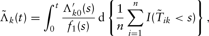
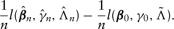
We will first prove that ${\hat{Λ}}_{kn} (t)$ is bounded almost surely as $n \to \infty$ for $k = 1, \dots, K$ . That is, ${\hat{Λ}}_{kn} (t)$ can be regarded as a bounded measure. By Helly's selection theorem and the compactness of the parameter space, for any subsequence of $({\hat{β}}_{n}, {\hat{γ}}_{n}, {\hat{Λ}}_{n})$ ${\hat{β}}_{n}$ converges to $β^{*}$ , ${\hat{γ}}_{n}$ converges to $γ^{*}$ , and ${\hat{Λ}}_{n}$ converges weekly to some $Λ^{*}$ on $[τ_{1}, τ_{2}]$ . The proof will be completed if we can show that $θ^{*} = θ_{0}$ . To establish the consistency of the estimators, we first define

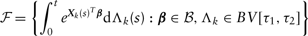
{\tilde{Λ}}_{k} (t) = \int_{0}^{t} \frac{Λ_{k 0}^{'} (s)}{f_{1} (s)} d \{\frac{1}{n} \sum_{i = 1}^{n} I ({\tilde{T}}_{ik} < s)\},

where $f_{1} (t)$ denotes the Radon–Nikodym derivative of $E {{\tilde{T}}_{ik} < t)}$ . We conclude that ${\tilde{Λ}}_{k} (t)$ converges uniformly to $Λ_{k 0} (t)$ with probability one for $t \in [τ_{1}, τ_{2}]$ in that $\frac{1}{n} \sum_{i = 1}^{n} I ({\tilde{T}}_{ik} < t) \to E {I ({\tilde{T}}_{ik} < t)}$ uniformly in $t$ with probability one as $n \to \infty$ . Let $BV [τ_{1}, τ_{2}]$ denote the functions whose total variation in $[τ_{1}, τ_{2}]$ are bounded by a given constant, and the class of functions

F = \{\int_{0}^{t} e^{X_{k} (s)^{T} β} d Λ_{k} (s) : β \in B, Λ_{k} \in BV [τ_{1}, τ_{2}]\}

be a Donsker class due to the fact that $F$ is a convex hull of functions ${I (t \geq s) e^{X_{k} (s)^{T} β}}$ . By conditions (A4) and (A5), we know that

\begin{matrix} \int_{b} \prod_{k = 1}^{K} {\{1 - exp [- G_{k} \{\int_{0}^{{\tilde{T}}_{k}} e^{X_{k} (s)^{T} β} d Λ_{k} (s) b\}]\}}^{Δ_{1 k}} \\ \times {[λ ({\tilde{T}}_{k}) e^{X_{ik} ({\tilde{T}}_{k})^{T} β} b_{i} G_{k}^{'} \{\int_{0}^{{\tilde{T}}_{k}} e^{X_{ik} (s)^{T} β} d Λ_{k} (s) b_{i}\}]}^{Δ_{2 k}} \\ \times exp {[- G_{k} \{\int_{0}^{{\tilde{T}}_{k}} e^{X_{k} (s)^{T} β} d Λ_{k} (s) b\}]}^{1 - Δ_{1 k}} p (b | γ) d b . \end{matrix}

is bounded away from zero. Therefore, $l (β_{0}, γ_{0}, \tilde{Λ})$ belongs to some Donsker class due to the preservation property of the Donsker class under the Lipschitz–continuous transformations. Then we can conclude that $| ℙ_{n} l (β_{0}, γ_{0}, \tilde{Λ}) - ℙ l (β_{0}, γ_{0}, \tilde{Λ}) |$ converges almost surely to $0$ as $n \to \infty$ . Since we denote $({\hat{β}}_{n}, {\hat{γ}}_{n}, {\hat{Λ}}_{n})$ as the maximum likelihood estimator, we have $ℙ_{n} l ({\hat{β}}_{n}, {\hat{γ}}_{n}, {\hat{Λ}}_{n}) > ℙ_{n} l (β_{0}, γ_{0}, \tilde{Λ})$ . Additionally, we know that $ℙ l (β_{0}, γ_{0}, \tilde{Λ})$ converges to $ℙ l (β_{0}, γ_{0}, Λ_{0})$ , which is finite. Therefore, we can conclude that $lim inf_{n} ℙ_{n} l ({\hat{β}}_{n}, {\hat{γ}}_{n}, \hat{Λ}) \geq O (1)$ . By following the conclusion of the Lemma 1, we know that

\begin{matrix} O (1) \leq lim inf_{n} ℙ_{n} l ({\hat{β}}_{n}, {\hat{γ}}_{n}, {\hat{Λ}}_{n}) \\ \leq lim sup_{n} ℙ_{n} log \{\int_{b} \prod_{k = 1}^{K} exp {[- G_{k} \{\int_{0}^{{\tilde{T}}_{k}} e^{X_{k} (s)^{T} {\hat{β}}_{n}} d {\hat{Λ}}_{kn} (s) b\}]}^{1 - Δ_{1 k} - Δ_{2 k}} p (b | {\hat{γ}}_{n}) d b\} \\ \leq - lim sup_{n} ℙ_{n} \sum_{k = 1}^{K} (1 - Δ_{1 k} - Δ_{2 k}) ρ_{0} {1 + {\hat{Λ}}_{kn} ({\tilde{T}}_{k})} + log (K) \\ \leq - lim sup_{n} ℙ_{n} \sum_{k = 1}^{K} (1 - Δ_{1 k} - Δ_{2 k}) ρ_{0} I ({\tilde{T}}_{k} = τ_{2}) {1 + {\hat{Λ}}_{kn} (τ_{2})} + log (K) . \end{matrix}

Hence, $lim sup_{n} ℙ_{n} \sum_{k = 1}^{K} (1 - Δ_{1 k} - Δ_{2 k}) ρ_{0} I ({\tilde{T}}_{k} = τ_{2}) {1 + {\hat{Λ}}_{kn} (τ_{2})} \leq O (1)$ , which implies $lim sup_{n} {\hat{Λ}}_{kn} (τ_{2}) < \infty$ with probability one. By Helly's selection theorem and the compactness of the parameter space, for any subsequence of ${\hat{θ}}_{n} = ({\hat{β}}_{n}, {\hat{γ}}_{n}, {\hat{Λ}}_{n})$ ${\hat{β}}_{n}$ converges to $β^{*}$ , $\hat{γ}$ converges to $γ^{*}$ , and ${\hat{Λ}}_{n}$ converges weekly to some $Λ^{*}$ on $[τ_{1}, τ_{2}]$ . Next, we consider the following difference of log-likelihood

\frac{1}{n} l ({\hat{β}}_{n}, {\hat{γ}}_{n}, {\hat{Λ}}_{n}) - \frac{1}{n} l (β_{0}, γ_{0}, \tilde{Λ}) .

By Lebesgue's theorem, we know that the left-hand side of the equation above converges to $E {l (β^{*}, γ^{*}, Λ^{*}) - l (β_{0}, γ_{0}, Λ_{0})}$ almost surely. Since the limit is the Kullback–Leibler divergence which is non-positive, we have $l (β^{*}, γ^{*}, Λ^{*}) = l (β_{0}, γ_{0}, Λ_{0})$ with probability one. Specially, for each $k$ , by choosing $Δ_{1 k} = Δ_{2 k} = 0$ and using condition (A3), we can show the identifiability of the model parameters. Therefore, we can conclude that $β^{*} = β_{0}, γ^{*} = γ_{0}$ and $Λ^{*} = Λ_{0}$ , which completes the proof.

Proof of Theorem 2.

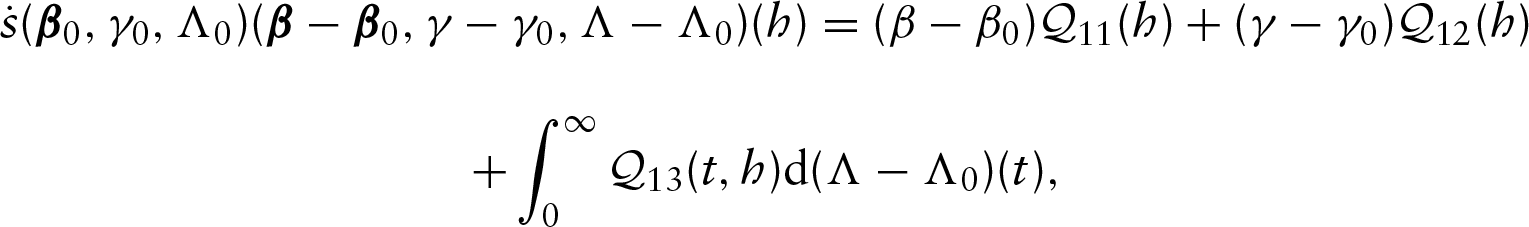
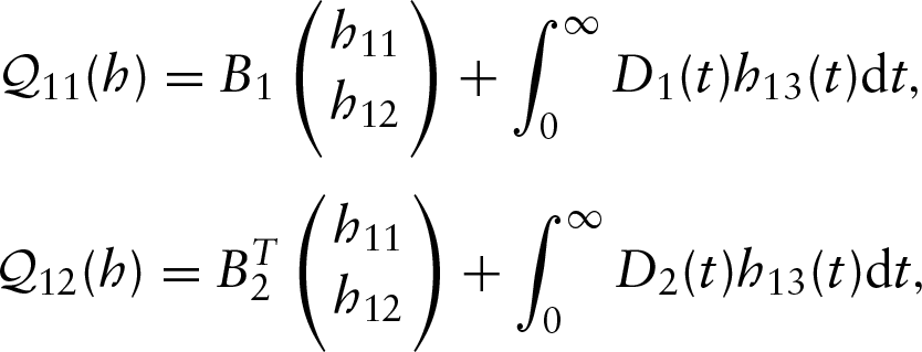
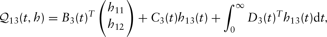
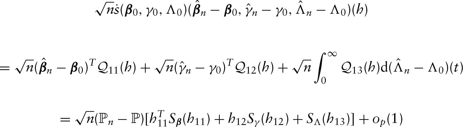
For the proof of this theorem, we propose to verify the four conditions stated in Theorem 2 of Murphy (1995) as has been done in Li et al. (2018). However, the techniques behind it are more complicated than those given in Li et al. (2018) due to the presence of frailty distribution in multivariate doubly censored data. Define $H = {h = (h_{11}, h_{12}, h_{13}) : h_{11} \in ℝ^{d} with ∥ h_{11} ∥_{1} < \infty, | h_{12} | < \infty, h_{13} = (h_{1} (t), \dots, h_{K} (t))$ $with h_{k} (t) \in BV [0, τ] for k = 1, \dots, K}$ . Consider parametric submodels $β_{ε} = β + ε h_{11}$ , $γ_{ε} = γ + ε h_{12}$ , and $Λ_{ε} (t) = (Λ_{1, ε} (t), \dots, Λ_{K, ε} (t))$ , where $Λ_{k, ε} (t) = Λ_{k} (t) + ε \int_{0}^{t} h_{k} (s) d s$ . Let $m (t) = \int_{0}^{t} e^{X_{ik} (s)^{T} β} d Λ_{k} (s) b_{i} .$ Therefore, the score functions along these submodels are given by

\begin{matrix} S_{n, β} (h_{11}) = \frac{1}{n} \frac{\partial l (β_{ε}, γ, Λ)}{\partial ε} |_{ε = 0} = \\ \frac{1}{n} \sum_{i = 1}^{n} L_{i} (θ, O)^{- 1} \int_{b_{i}} \prod_{k = 1}^{K} A_{ik} (β, Λ, O) \sum_{k = 1}^{K} {\int_{0}^{{\tilde{T}}_{ik}} e^{X_{ik} (s)^{T} β} X_{ik} (s) d Λ (s) b_{i} \\ \times [\frac{Δ_{1 ik} exp (- G (m ({\tilde{T}}_{ik}))) G_{k}^{'} (m ({\tilde{T}}_{ik}))}{1 - exp (- G_{k} (m ({\tilde{T}}_{ik})))} + Δ_{2 ik} \frac{G^{″} (m ({\tilde{T}}_{ik}))}{G_{k}^{'} (m ({\tilde{T}}_{ik}))} - (1 - Δ_{1 ik}) G_{k}^{'} (m ({\tilde{T}}_{ik}))] \\ + Δ_{2 ik} X_{ik} ({\tilde{T}}_{ik})} p (b_{i} | γ) d b_{i} h_{11}, \\ S_{n, Λ_{k}} (h_{k}) = \frac{1}{n} \frac{\partial l (β, γ, Λ_{ε})}{\partial ε} |_{ε = 0} = \\ \frac{1}{n} \sum_{i = 1}^{n} L_{i} (θ, O)^{- 1} \int_{b_{i}} \prod_{k = 1}^{K} A_{ik} (θ, Λ, O) \sum_{k = 1}^{K} {\int_{0}^{{\tilde{T}}_{ik}} e^{X_{ik} (s)^{T} β} h_{k} (s) d s b_{i} \\ \times [\frac{Δ_{1 ik} exp (- G (m ({\tilde{T}}_{ik}))) G_{k}^{'} (m ({\tilde{T}}_{ik}))}{1 - exp (- G_{k} (m ({\tilde{T}}_{ik})))} \\ + Δ_{2 ik} \frac{G^{″} (m ({\tilde{T}}_{ik}))}{G_{k}^{'} (m ({\tilde{T}}_{ik}))} - (1 - Δ_{1 ik}) G_{k}^{'} (m ({\tilde{T}}_{ik}))] + Δ_{2 ik} h_{k} ({\tilde{T}}_{ik})} p (b_{i} | γ) d b_{i}, \end{matrix}

and

S_{n, η} (h_{12}) = \frac{1}{n} \frac{\partial l (β, γ_{ε}, Λ)}{\partial ε} |_{ε = 0} = \frac{1}{n} \sum_{i = 1}^{n} L_{i} (θ, O)^{- 1} \int_{b_{i}} \prod_{k = 1}^{K} A_{ik} (θ, O) \partial p (b_{i} | γ) / \partial γ d b_{i} h_{12},

where $L_{i} (θ, O) = \int_{b_{i}} \prod_{k = 1}^{K} A_{ik} (β, Λ, O) p (b_{i} | γ) d b_{i}$ and

A_{ik} (β, Λ, O) = {\{1 - S_{k} ({\tilde{t}}_{ik})\}}^{Δ_{1 ik}} f_{k} ({\tilde{T}}_{ik})^{Δ_{ik}} S_{k} ({\tilde{T}}_{ik})^{1 - Δ_{1 ik} - Δ_{2 ik}} .

Denote $S_{n} (β, γ, Λ) (h) = S_{n, β} (h_{11}) + S_{n, η} (h_{12}) + S_{n, Λ} (h_{13})$ , where $S_{n, Λ} (h_{13}) = \sum_{k = 1}^{K} S_{n, Λ_{k}} (h_{k})$ . Furthermore, we define the limit map $s : (β, γ, Λ) \to l^{\infty} (H)$ as $s (β, γ, Λ) = S_{β} (h_{11}) + S_{γ} (h_{12}) + S_{Λ} (h_{13})$ , where the linear functionals $S_{β} (h_{11})$ , $S_{γ} (h_{12})$ and $S_{Λ_{k}} (h_{k})$ are obtained by replacing the empirical sum by the expectation and $S_{Λ} (h_{13}) = \sum_{k = 1}^{K} S_{Λ_{k}} (h_{k})$ . Clearly, $S_{n} ({\hat{β}}_{n}, {\hat{γ}}_{n}, {\hat{Λ}}_{n}) (h) = 0$ and $s (β_{0}, γ_{0}, Λ_{0}) (h) = 0$ . The desired asymptotic normality will be established if we can verify the four conditions stated in Theorem 2 of Murphy (1995). The first condition that $\sqrt{n} (S_{n} (β_{0}, γ_{0}, Λ_{0}) (h) - s (β_{0}, γ_{0}, Λ_{0}) (h))$ converges weakly to a tight Gaussian process on $l^{\infty} (H)$ holds since $l (β_{0}, γ_{0}, Λ_{0})$ belongs to a Donsker class and $S_{β} (h_{11})$ , $S_{γ} (h_{12})$ and $S_{Λ} (h_{13})$ are bounded Lipschitz functionals with respect to $H .$ By Proposition 1 in the Appendix of Bickel et al. (1993), we can show that $s (β, γ, Λ)$ is Fr $\overset{´}{e}$ chet differentiable. The approximation condition can be proved using Lemma 3.3.5 in van der Vaart and Wellner (1996). Let $\dot{s} (β_{0}, γ_{0}, Λ_{0}) (β - β_{0}, γ - γ_{0}, Λ - Λ_{0}) (h)$ denote the corresponding Fr $\overset{´}{e}$ chet derivative of $s (β, γ, Λ)$ at $(β_{0}, γ_{0}, Λ_{0})$ . After some algebra, we can have

\begin{matrix} \dot{s} (β_{0}, γ_{0}, Λ_{0}) (β - β_{0}, γ - γ_{0}, Λ - Λ_{0}) (h) = (β - β_{0}) Q_{11} (h) + (γ - γ_{0}) Q_{12} (h) \\ + \int_{0}^{\infty} Q_{13} (t, h) d (Λ - Λ_{0}) (t), \end{matrix}

where

\begin{matrix} Q_{11} (h) = B_{1} (\begin{matrix} h_{11} \\ h_{12} \end{matrix}) + \int_{0}^{\infty} D_{1} (t) h_{13} (t) d t, \\ Q_{12} (h) = B_{2}^{T} (\begin{matrix} h_{11} \\ h_{12} \end{matrix}) + \int_{0}^{\infty} D_{2} (t) h_{13} (t) d t, \end{matrix}

and

Q_{13} (t, h) = B_{3} (t)^{T} (\begin{matrix} h_{11} \\ h_{12} \end{matrix}) + C_{3} (t) h_{13} (t) + \int_{0}^{\infty} D_{3} (t)^{T} h_{13} (t) d t,

where $B_{1}$ is a $d \times (d + 1)$ matrix, $B_{2}$ and $B_{3} (t)$ are $(d + 1)$ -dimensional vectors, $D_{1} (t)$ , $C_{3} (t)$ and $D_{2} (t)$ are scalar functions and $D_{3} (t)$ is a $K$ -dimensional vector function.

Therefore, the invertibility of $\dot{s} (β_{0}, γ_{0}, Λ_{0})$ is equivalent to the invertibility of the continuous linear operator $Q (h) = (Q_{11} (h), Q_{12} (h), Q_{13} (t, h))$ for any $t$ . It suffices to prove that $Q (h)$ is a one-to-one map (Rudin 1973). Note that if $Q (h) = 0,$ then $\dot{s} (β_{0}, γ_{0}, Λ_{0}) (β - β_{0}, γ - γ_{0}, Λ - Λ_{0}) [h] = 0$ for any $(β, γ, Λ)$ in the neighbourhood of $(β_{0}, γ_{0}, Λ_{0}) .$ We choose $β - β_{0} = ε h_{11}$ , $γ - γ_{0} = ε h_{12}$ and $Λ (t) - Λ_{0} (t) = ε \int_{0}^{t} h_{13} (s) d Λ (s) .$ By the definition of $\dot{s} (β_{0}, γ_{0}, Λ_{0}) (h),$ $\dot{s} (β_{0}, γ_{0}, Λ_{0}) (h) = ε ℙ (h_{11}^{T} S_{β} (h_{11}) + h_{12} S_{γ} (h_{12}) + S_{Λ} (h_{13}))^{2} = 0 .$ Thus, $h_{11}^{T} S_{β} (h_{11}) + h_{12} S_{γ} (h_{12}) + S_{Λ} (h_{13}) = 0$ almost surely. After some algebra, we can obtain $h_{11} = 0, h_{12} = 0$ and $h_{13} \equiv 0$ by condition (A3).

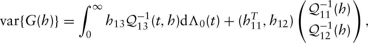
Since it has already been shown that $Q (h) = (Q_{11} (h), Q_{12} (h), Q_{13} (h))$ is invertible, the asymptotic property stated in Theorem 2 now follows from Theorem 2 of Murphy (1995). Furthermore,

\begin{matrix} \sqrt{n} \dot{s} (β_{0}, γ_{0}, Λ_{0}) ({\hat{β}}_{n} - β_{0}, {\hat{γ}}_{n} - γ_{0}, {\hat{Λ}}_{n} - Λ_{0}) (h) \\ = \sqrt{n} ({\hat{β}}_{n} - β_{0})^{T} Q_{11} (h) + \sqrt{n} ({\hat{γ}}_{n} - γ_{0})^{T} Q_{12} (h) + \sqrt{n} \int_{0}^{\infty} Q_{13} (h) d ({\hat{Λ}}_{n} - Λ_{0}) (t) \\ = \sqrt{n} (ℙ_{n} - ℙ) [h_{11}^{T} S_{β} (h_{11}) + h_{12} S_{γ} (h_{12}) + S_{Λ} (h_{13})] + o_{p} (1) \end{matrix}

uniformly in $h = (h_{11}, h_{12}, h_{13}) .$ Therefore, $\sqrt{n} {({\hat{β}}_{n}, {\hat{γ}}_{n}, {\hat{Λ}}_{n}) - (β_{0}, γ_{0}, Λ_{0})}$ converges in distribution to a tight Gaussian process $G = {\dot{s} (β_{0}, γ_{0}, Λ_{0})}^{- 1} G^{*}$ , whose variance is given by

var {G (h)} = \int_{0}^{\infty} h_{13} Q_{13}^{- 1} (t, h) d Λ_{0} (t) + (h_{11}^{T}, h_{12}) (\begin{matrix} Q_{11}^{- 1} (h) \\ Q_{12}^{- 1} (h) \end{matrix}),

where $Q^{- 1} (h) = (Q_{11}^{- 1} (h), Q_{12}^{- 1} (h), Q_{13}^{- 1} (h))$ is the inverse of $Q (h)$ . Note that $({\hat{β}}_{n}, {\hat{γ}}_{n})$ is an asymptotically linear estimator for $(β_{0}, γ_{0})$ , and its influence function belongs to the space spanned by the score functions, which indicates $({\hat{β}}_{n}, {\hat{γ}}_{n})$ is semiparametrically efficient (Bickel et al. 1993).

Footnotes

Acknowledgments

This work was partly supported by the National Nature Science Foundation of China grant nos. 11671274, 11731011 and 11671168, the Support Project of High-level Teachers in Beijing Municipal Universities in the Period of 13th Five-year Plan grant CIT & TCD 201804078, the Capacity Building for Sci-Tech Innovation-Fundamental Scientific Research Funds grant 025185305000/204, the Youth Innovative Research Team of Capital Normal University, and the Science and Technology Developing Plan of Jilin Province grant 20170101061 J.C.

Declaration of conflicting interests

The authors declared no potential conflicts of interest with respect to the research, authorship and/or publication of this article.

Funding

References

Bickel

, Klaassen

CAJ

, Ritov

Wellner

(1993) Efficient and Adaptive Estimation for Semiparametric Models . Baltimore, MD: Johns Hopkins University Press.

Cai

Cheng

(2004) Semiparametric regression analysis for doubly censored data. Biometrika , 91, 277–90.

Matsouaka

, Li

Cai

(2014) Evaluating marker-guided treatment selection strategies. Biometrics , 70, 489–99.

Chang

(1990) Weak convergence of a self-consistent estimator of the survival function with doubly censored data. The Annals of Statistics , 18, 391–404.

Chang

Yang

(1987) Strong consistency of a nonparametric estimator of the survival function with doubly censored data. The Annals of Statistics , 15, 1536–47.

Gehan

(1965) A generalized two-sample Wilcoxon test for doubly censored data. Biometrika , 52, 650–53.

Goggins

Finkelstein

(2000) A pro- portional hazards model for multivariate interval-censored failure time data. Biometrics , 56, 940–43.

Gómez

, Calle

, Oller

Langohr

(2009) Tutorial on methods for interval- censored data and their implementation in R. Statistical Modelling , 9, 259–97.

Guo

Rodriguez

(1992) Estimating a multivariate proportional hazards model for clustered data using the EM algorithm, with an application to child survival in Guatemala. Journal of the American Statistical Association , 87, 969–76.

10.

Hammer

, Squires

, Hughes

, Grimes

, Demeter

, Currier

, Eron

, Feinberg

, Balfour

, Deyton

, Chodakewitz

Fischl

(1997) A controlled trial of two nucleoside analogues plus indinavir in persons with human immunodeficiency virus infection and CD4 cell counts of 200 per cubic millimeter or less. New England Journal of Medicine , 337, 725–33.

11.

Kim

, Kim

Jang

(2010) Asymptotic properties of the maximum likelihood estimator for the proportional hazards model with doubly censored data. Journal of Multivariate Analysis , 101, 1339–51.

12.

Kim

, Kim

Jang

(2013) An EM algorithm for the proportional hazards model with doubly censored data. Computational Statistics and Data Analysis , 57, 41–51.

13.

Komarek

Lesaffre

(2006) Bayesian semi-parametric accelerated failure time model for paired doubly-interval-censored data. Statistical Modelling , 6, 3–22.

14.

Kosorok

Lee

Fine

(2004) Robust inference for univariate proportional hazards frailty regression models. The Annals of Statistics , 32, 1448–91.

15.

Zhou

Sun

(2017) Regression analysis of bivariate current status data under the proportional hazards model. The Canadian Journal of Statistics , 45, 410–24.

16.

Wang

Sun

(2017) Regression analysis of current status data in the presence of dependent censoring with applications to tumorigenicity. Computational Statistics and Data Analysis , 110, 75–86.

17.

Wang

Sun

. (2018) A class of semiparametric transformation models for doubly censored failure time data. Scandinavian Journal of Statistics . doi: 10.1111/sjos.12319.

18.

Lin

Ying

(1994) Semiparametric analysis of the additive risk model. Biometrika , 81, 61–71.

19.

McMahan

, Wang

Tebbs

(2013) Regression analysis for current status data using the EM algorithm. Statistics in Medicine , 32, 4452–66.

20.

Murphy

(1995) Asymptotic theory for the frailty model. The Annals of Statistics , 23, 182–98.

21.

Mykland

Ren

(1996) Algorithms for computing self-consistent and maximum likelihood estimators with doubly censored data. The Annals of Statistics , 24, 1740–64.

22.

Nelson

Lipsitz

Fitzmaurice

Ibrahim

Parzen

Strawderman

(2006) Use of the probability integral transformation to fit nonlinear mixed-effects models with nonnormal random effects. Journal of Computational and Graphical Statistics , 15, 39–57.

23.

Rudin W (1973) Functional Analysis . New York, NY: McGraw-Hill.

24.

Scharfstein

Robins

(2002) Estimation of the failure time distribution in the presence of informative censoring. Biometrika , 89, 617–34.

25.

Siannis

Copas

(2005) Sensitivity analysis for informative censoring in parametric survival models. Biostatistics , 6, 77–91.

26.

Wang

(2016) Semiparametric efficient estimation for shared-frailty models with doubly censored clustered data. The Annals of Statistics , 44, 1298–1331.

27.

Sun

(1995) Empirical estimation of a distribution function with truncated and doubly interval-censored data and its application to AIDS studies. Biometrics , 51, 1096–1104.

28.

Sun

(2006) The Statistical Analysis of Interval-censored Failure Time Data . New York, NY: Springer.

29.

Sun

Wang

Sun

(2016) Estimation of the association for bivariate interval-censored failure time data. Scandinavian Journal of Statistics , 33, 637–49.

30.

van der Vaart

Wellner

(1996) Weak Convergence and Empirical Processes . New York, NY: Springer.

31.

Wang

McMahan

(2015) Regression analysis of bivariate current status data under the gamma-frailty proportional hazards model using the EM algorithm. Computational Statistics and Data Analysis , 83, 140–50.

32.

Wang

Ding

(2000) On assessing the association for bivariate current status data. Biometrika , 87, 879–93.

33.

Wei

Lin

Weissfeld

(1989) Regression analysis of multivariate incomplete failure time data by modelling marginal distributions. Journal of the American Statistical Association , 84, 1065–73.

34.

Wen

Chen

(2011) Nonparametric maximum likelihood analysis of clustered current status data with the gamma-frailty Cox model. Computational Statistics and Data Analysis , 55, 1053–60.

35.

Zeng

Chen

Ibrahim

(2009) Gamma frailty transformation models for multivariate survival times. Biometrika , 96, 277–91.

36.

Zeng

Lin

(2008) Semiparametric transformation models with random effects for clustered failure time data. Statistica Sinica , 18, 355–77.

37.

Zeng

Mao

Lin

(2016) Maximum likelihood estimation for semiparametric transformation models with interval-censored data. Biometrika , 103, 253–71.

38.

Zhang

(1996) Linear regression with doubly censored data. The Annals of Statistics , 24, 2720–43.

39.

Zhang

Jamshidian

(2004) On algorithms for the nonparametric maximum likelihood estimator of the failure function with censored data. Journal of Computational and Graphical Statistics , 13, 123–40.

40.

Zhou

Sun

(2017) A sieve semiparametric maximum likelihood approach for regression analysis of bivariate interval-censored failure time data. Journal of the American Statistical Association , 112, 664–72.