
Abstract
We propose and estimate an alternating renewal model describing the propagation of anomalies in a backbone internet network in the United States. Internet anomalies, either caused by equipment malfunction, news events or malicious attacks, have been a focus of research in network engineering since the advent of the internet over 30 years ago. This article contributes to the understanding of statistical properties of the times between the arrivals of the anomalies, their duration and stochastic structure. Anomalous, or active, time periods are modelled as periods containing clusters or 1s, where 1 indicates a presence of an anomaly. The inactive periods consisting entirely of 0s dominate the 0–1 time series in every link. Since the active periods contain 0s, a separation parameter is introduced and estimated jointly with all other parameters of the model. Our statistical analysis shows that the integer-valued separation parameter and five other non-negative, scalar parameters satisfactorily describe all statistical properties of the observed 0–1 series.
Introduction
Research presented in this article is motivated by the need to understand statistical properties of the propagation of anomalies observed in the internet traffic. We study data obtained from a nationwide network linking major hubs in the United States. There are many types of anomalies including Distributed Denial of Service attacks or link failures, but this article is not concerned with their detection or classification. Our aim is to construct a statistical model that describes important aspects of the movement of anomalies across the network. We use a suitable database created by other researchers.
There are many potential benefits to understanding statistical properties of the propagation of anomalies over a nationwide network over a long period of time. One is to facilitate the design of network simulators, which are used to validate computer networks before deployment. Another application is to plan the provisioning of hardware and software resources. There has been extensive research on anomaly detection, literally hundreds of articles, so we do not even attempt a review. Chandolla et al. (2009) provide a comprehensive survey of anomaly detection methods in various applications. Tsai et al. (2009) review 55 studies on intrusion detection in internet networks. Bhuyan et al. (2014) comprehensively survey general network anomaly detection methods, systems, and tools, in terms of the underlying computational techniques, while Liao et al. (2013) summarize the network intrusion detection with respect to different network scenarios, from the perspective of system deployments, timeliness requirements, data sources and detection strategies. The anomaly detection techniques and systems in specific network scenarios, for example, wireless sensor networks, Xie et al. (2011), and internet of things, Zarpelao et al. (2017), have been thoroughly reviewed with respect to the distinct characteristics of their network anomalies and detection requirements. Paschalidis and Smaragdakis (2009) consider a spatio-temporal framework for anomaly detection. Kallitsis et al. (2016) describe a hardware–software framework for attack detection that operates on live internet traffic.
In contrast to extensive research on anomaly detection, there is little work on quantitatively describing the propagation of anomalies through a network. A statistical model for anomaly occurrence and duration could enhance network design and performance and help improve network intrusion detection systems. This low level of understanding of the stochastic structure of anomalous traffic must also be contrasted with a profound understanding of the structure of regular traffic over the internet and its subnetworks. The groundbreaking work of Leland et al. (1994) discovered the self-similar nature of such traffic, many elaborations on their work are presented in Park andWillinger (2000). Most models for regular traffic over relatively short time intervals postulate a fractal or multi-fractal structure with normal marginal distributions. More recent references and a comprehensive network-wide predictive model are given in, for example, Vaughan et al. (2013). We show that in contrast to the self-similar, hence strongly dependent, Gaussian time series models used to describe regular traffic, important aspects of anomalous traffic can be well described by independent, but highly non-Gaussian random variables. We build on the work of Bandara et al. (2014) and Kokoszka et al. (2020). Bandara et al. (2014) constructed and described the database we use and presented a preliminary statistical model based on exponential and normal distributions. Using probabilistic and statistical analysis, Kokoszka et al. (2020) showed that light-tailed distributions are not appropriate to describe times between the arrivals of anomalies, and one must use point processes with heavy-tailed interarrival times. In this article, we present a model not just for the times of arrivals of anomalies, but also for their duration and structure.
The remainder of the article is organized as follows. In Section 2, we introduce the database of Internet2 anomalies used and our modelling approach. Section 3 is dedicated to exploration of statistical properties of the data and model formulation. Building on Section 3, we compute model likelihood in Section 4 and estimate model parameters. Section 5 is dedicated to the study of the distribution of the waiting time until the arrival of the next anomaly. We conclude with Section 6, where we discuss the limits of our approach and possible future work.
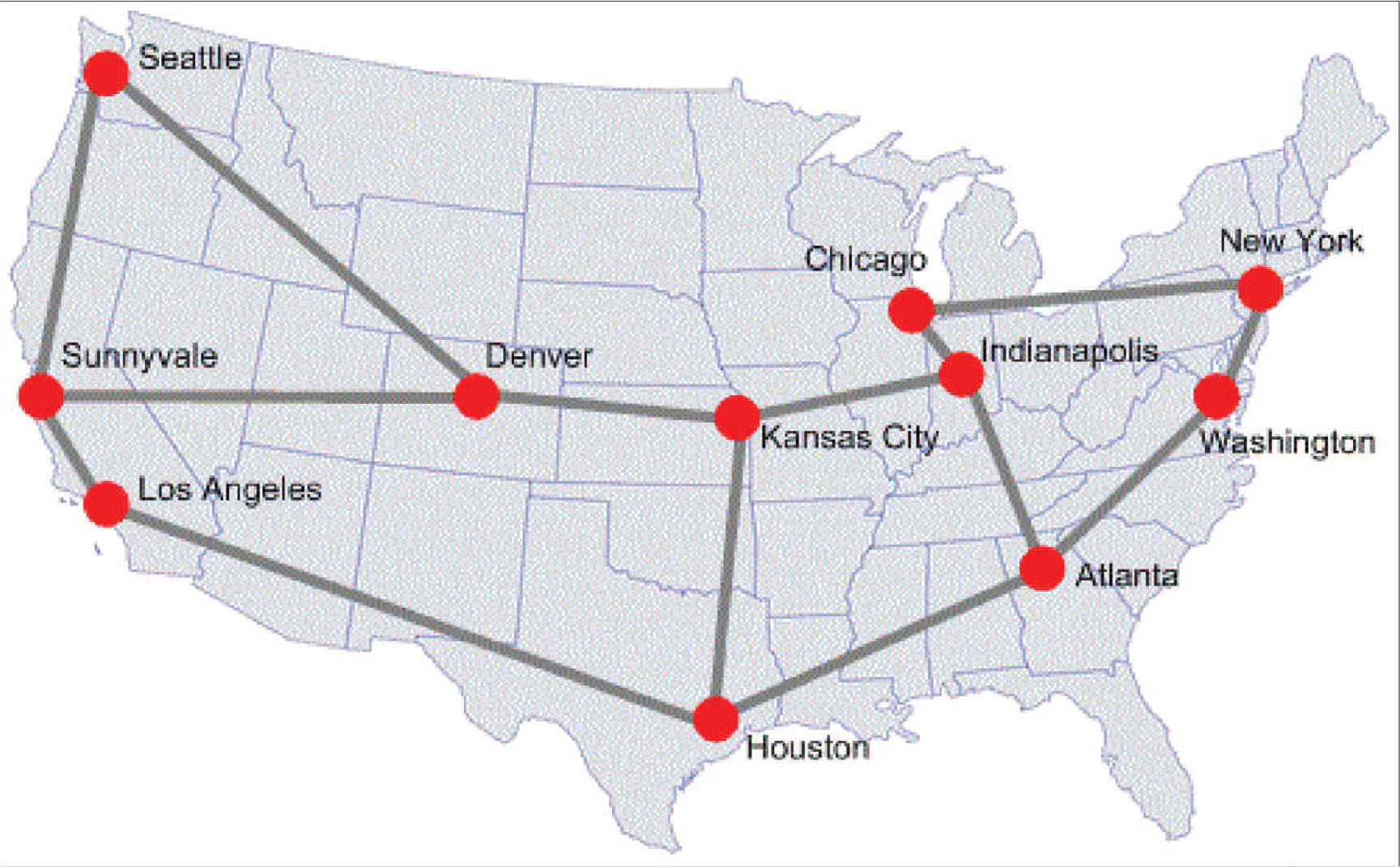
We use the database constructed by Bandara et al. (2014) who applied a frequency domain filter to extract time periods of unusually high traffic. Bandara et al. (2014) used traffic measured at the links of the Internet2 network shown in Figure 1 over the period of 50 weeks starting 16 October 2005. Their approach treats periodic and noise components of the measured traffic as usual traffic without anomalies. To extract the anomalies, the 20 largest Fourier components that capture about
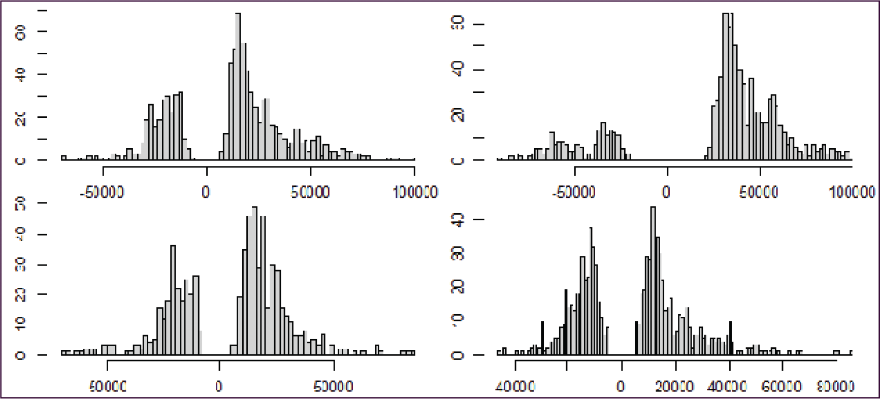
Histograms of the detrended values that are considered anomalous; top-left: incoming Atlanta–Houston, top-right incoming Chicago–Indianapolis, bottom-left: outgoing Denver–St. Louis, bottom-right: the outgoing Houston–Los Angeles
Histograms of the detrended values that are considered anomalous; top-left: incoming Atlanta–Houston, top-right incoming Chicago–Indianapolis, bottom-left: outgoing Denver–St. Louis, bottom-right: the outgoing Houston–Los Angeles
Bandara et al. (2014) treat a group of consecutive 1s as a single anomaly, which ends when a 0 occurs. However, examination of the data shows that very often there is a break of just one or two 0s before the next 1. It is reasonable to assume that two strings of 1s separated by a few 0s correspond to a single anomalous event. The issue is then how big a separation should be used to ensure optimal modelling. Using the separation of one recovers the original classification of Bandara et al. (2014). The database does not identify the hundreds of anomalies in the various links by associating them to some exogenously recorded events. We use statistical modelling to determine which separation level leads to a model most likely to explain the observed behaviour of the data.
The data are binary and hence can be modelled as a realization of a random sequence,
Since for each link our data begin with 0, we assume that we start in the middle of an inactive period. For mathematical consistency, we assume that
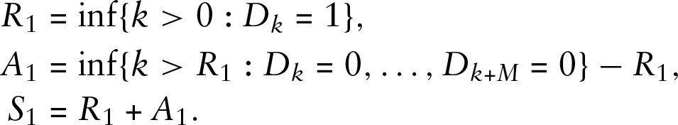
We see that
To illustrate, consider the following (fictitious) data string:

Setting,
Observe that
In the next section, we study distributional and dependence properties of the above model and propose a suitable statistical model.
The modelling approach outlined above can be described as an alternating renewal process. A good introduction to models of this type is given in Section 3.7 of Ross (1996). However, as we will see in Section 3, the commonly used exponential regeneration times are not suitable for the internet anomaly data.
We first analyse the dependence structure of the segments
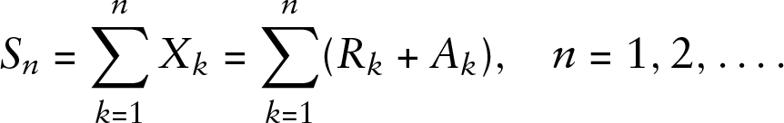
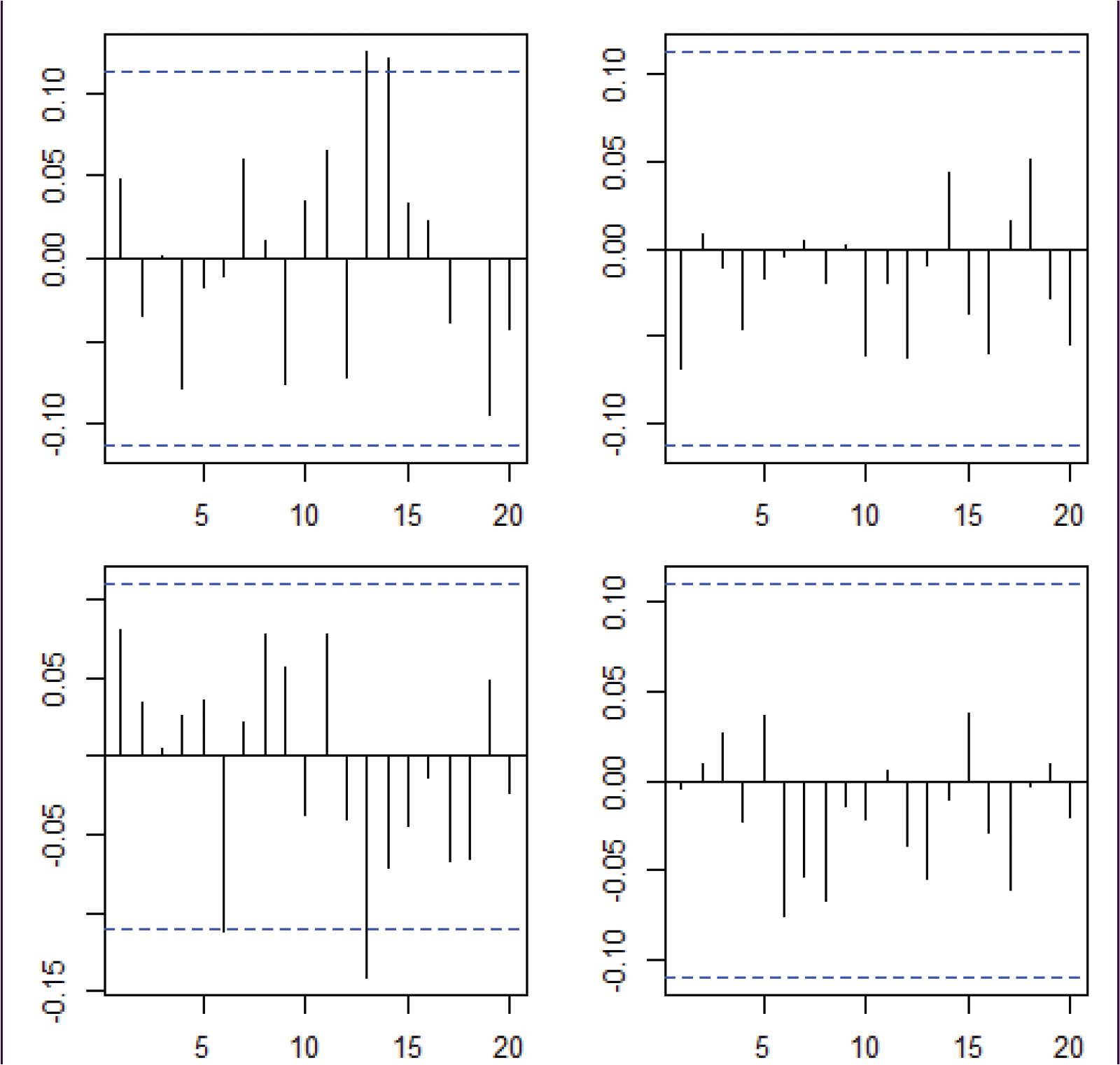
Figure 3 presents plots of the sample autocorrelations of the time-series
Autocorrelation of lengths of active (left) and inactive (right) periods for the Atlanta
Houston link for
. Top panels are for incoming anomalies, bottom for outgoing anomalies. The plots do not suggest any significant autocorrelations. The plots for different values of
look similar
Autocorrelation of lengths of active (left) and inactive (right) periods for the Atlanta
Houston link for
. Top panels are for incoming anomalies, bottom for outgoing anomalies. The plots do not suggest any significant autocorrelations. The plots for different values of
look similar
We begin by finding a family of distributions suitable for modelling the length of the inactive periods, the

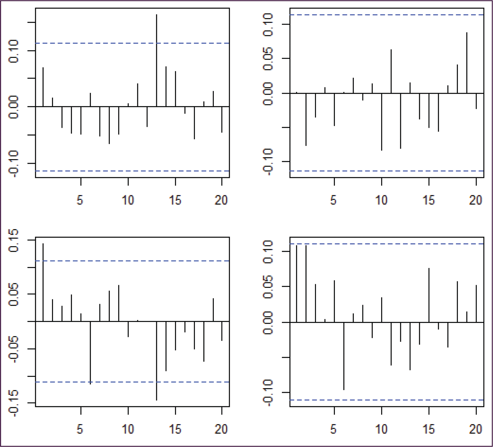
Autocorrelations of natural logarithms of the inputs described in the caption of Figure 3
where

Note that by taking
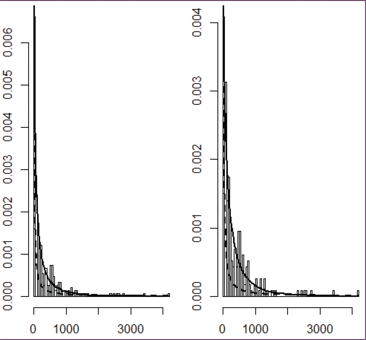
Histograms of the lengths of inactive periods shifted by
(left) and
(right), with the black line being the fitted PPS density, and the dotted line the fitted Pareto density for the Chicago
NYC link. The PPS density provides a much better fit for the middle portion of the distribution that the Pareto density
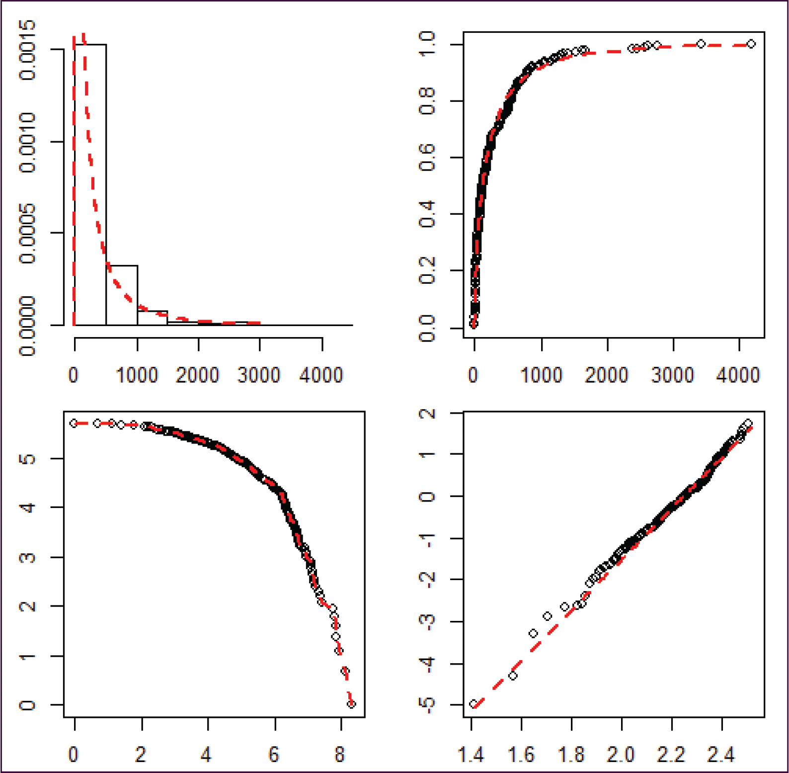
Diagnostic plots visualizing the goodness of fit of the PPS distribution to the data for
for the Atlanta
Houston link, and
. The first plot gives the fitted PPS density. The second compares the fitted PPS cdf to the empirical cdf. The third is a log-log rank plot which determines tail behaviour (if
has a Pareto tail, the line should be straight). The last plot is a double log rank plot which indicates the overall goodness of the data to the PPS distribution
We now turn to a model for the active periods. In this case, the discrete Pareto distribution fits the data fairly well visually, as evidenced by Figure 7. However, a potential issue with fitting a Pareto distribution to the active periods is that the maximum observed value can be relatively small for small

Histograms of the lengths of active periods for
and
for the Chicago
NYC link. The black line is the fitted mixed geometric distribution. The dashed line is the Pareto distribution
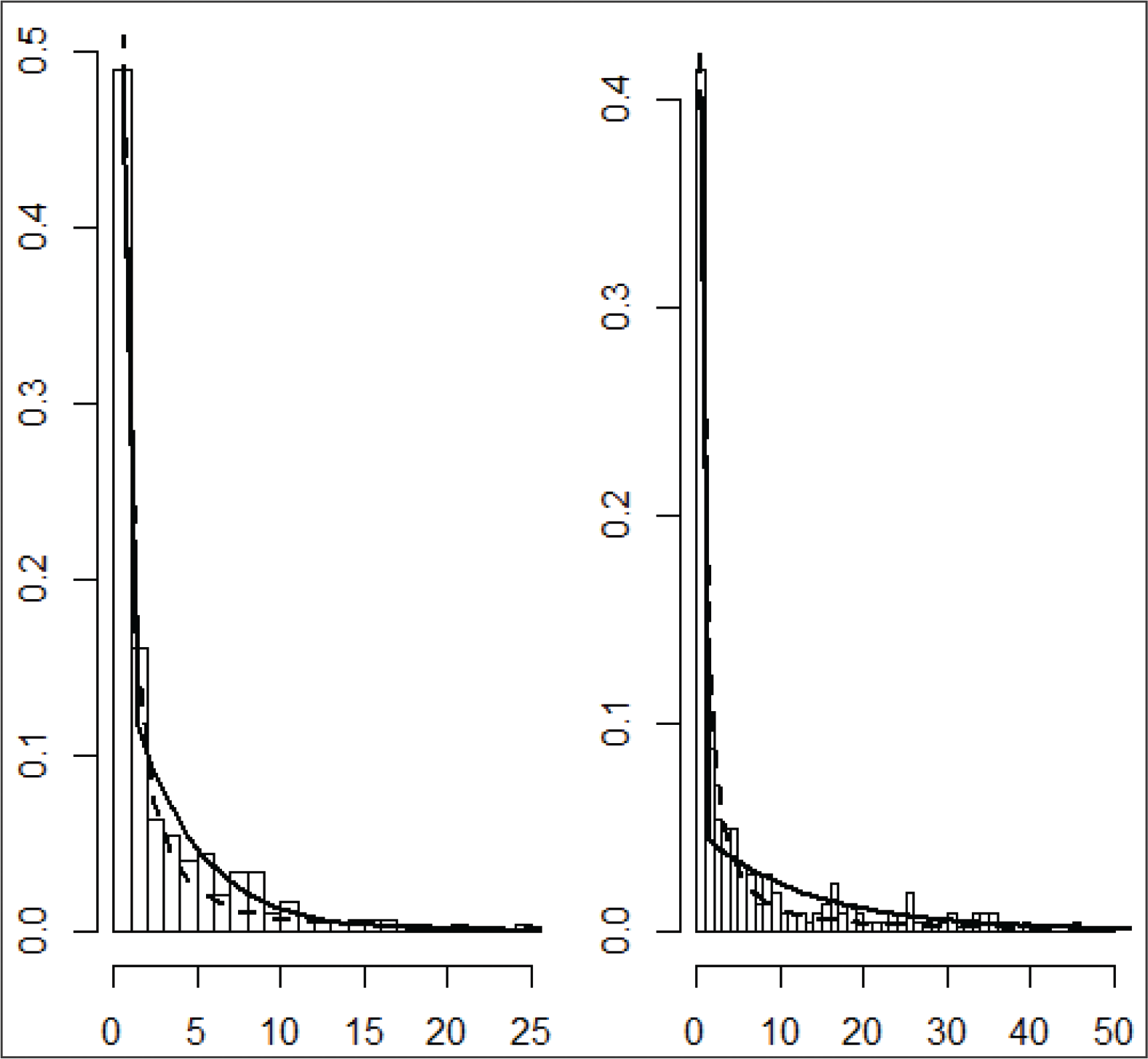
This distribution, as evidenced by Figure 8, provides a good fit for the data. In addition, the third panel, the log-log rank plot, indicates that the data do not follow a power law, and so the Pareto distribution is inappropriate.
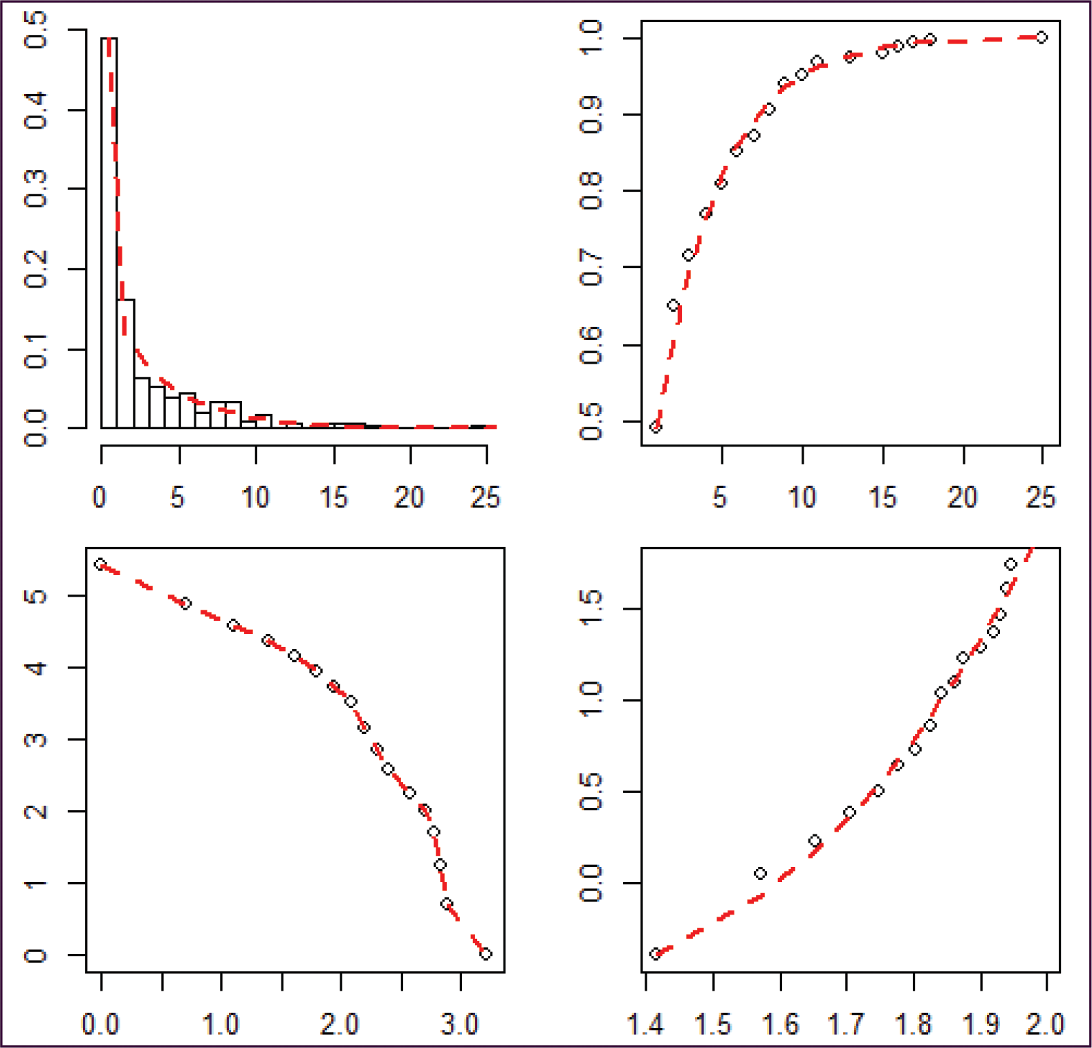
Diagnostic plots visualizing the goodness of fit of the PPS distribution to the data for
for the Atlanta
Houston link, and
. The first plot shows the fitted mixed geometric density. The second compares the fitted mixed geometric cdf to the empirical cdf. The third is a log-log rank plot which determines tail behaviour (if
has a Pareto tail, the line should be straight). The last plot is a double log rank plot which indicates the overall goodness of the data to the mixed geometric distribution
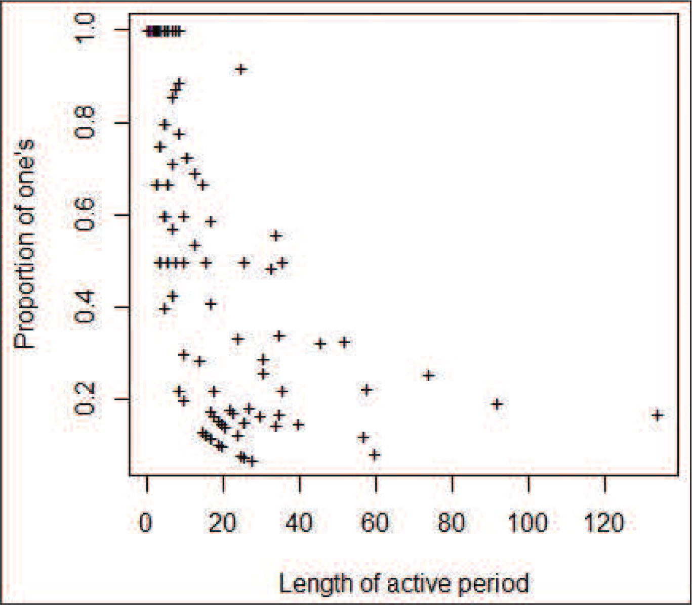
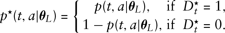
The remaining piece needed to model the binary string is to model the behaviour of the string during its active periods. Figure 9 shows evidence of a relationship between the length of the active period and the proportion of one's seen during the active period, which is something that should be taken into account. By the construction of the process, we define that the active periods begin after a one has been observed, so it follows that the first element of the string during an active period is a one. The high proportion of one's thus follows from construction combined with the fact that there are many anomalies that last less than five minutes. As the length of the active period increases, the proportion of one's decreases, which can also be attributed to how the model is constructed, especially for larger values of

Plot of the proportion of one's during an active period against the length of the active period for the Atlanta
Houston link with
where we note that
With all components of the statistical model in place, we turn in the next section to the computation of the likelihood function and parameter estimation.
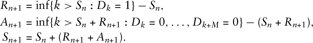
To derive the model likelihood, we use the recursions introduced in Section 2 together with the independence properties and distributional models proposed in Section 3. The components of the parameter vector
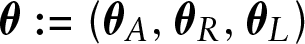
are defined by

To understand the principle of constructing the likelihood function, let us consider the toy example of Section 2. Denote by

Then,
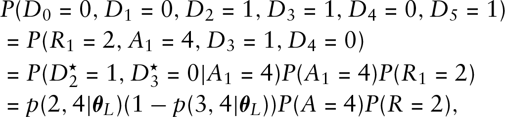
where
because the active period of length 2 has two 1s, which must occur with probability one by construction. For the third interarrival period,

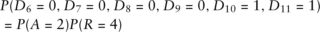
Finally, we have the remainder term,

The probabilities
We now specify likelihood in the general case. Let
For each
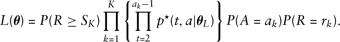
Observe that

with
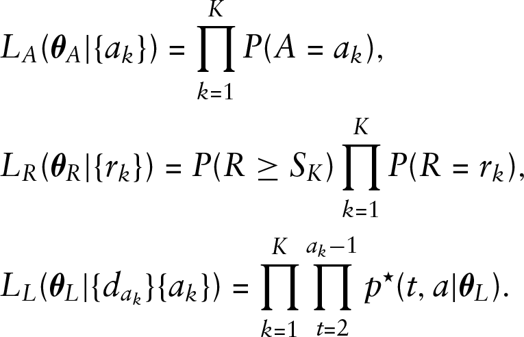
This implies that performing maximum likelihood estimation can be achieved by performing partial likelihood estimation on each individual component, easing the complexity of an optimization routine.
Note that in general the final observation of the data will not be the end of the last interrenewal, so for the likelihood to be complete, we need to consider the likelihood of the observations
In fact, explicit formulas for the MLEs of the parameters of the distribution can be derived. Consider the distribution

and note that here we recover our original distribution by setting
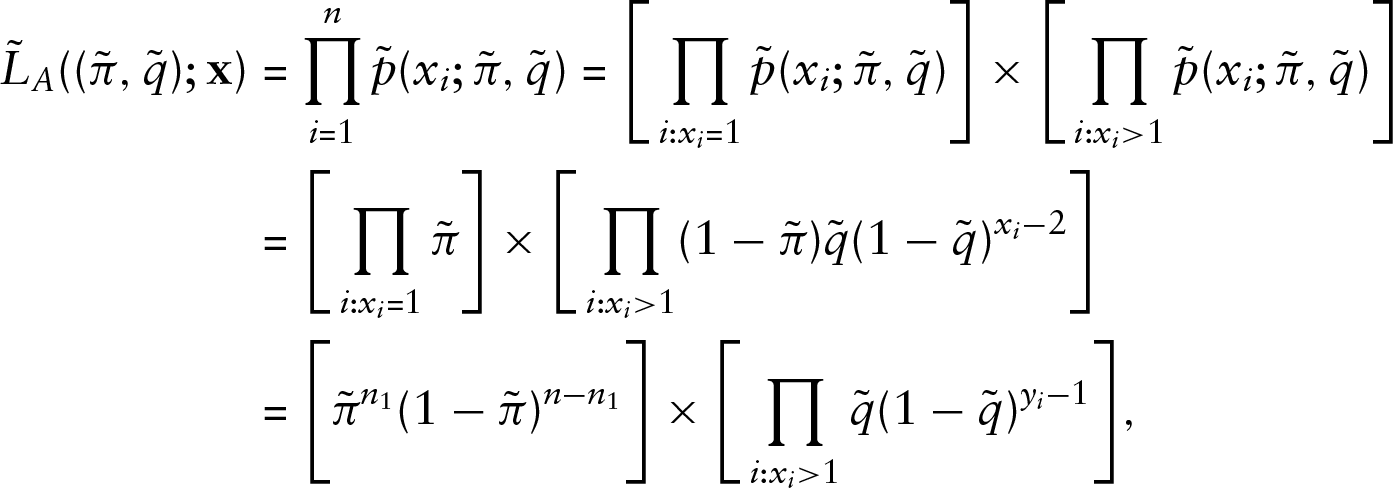
where we define
Noting that the first term is the likelihood function of a binary random variable, we know that
Lastly, we define
that is,
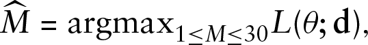
The optimal values of
and parameter estimates for these values for each link for the incoming direction
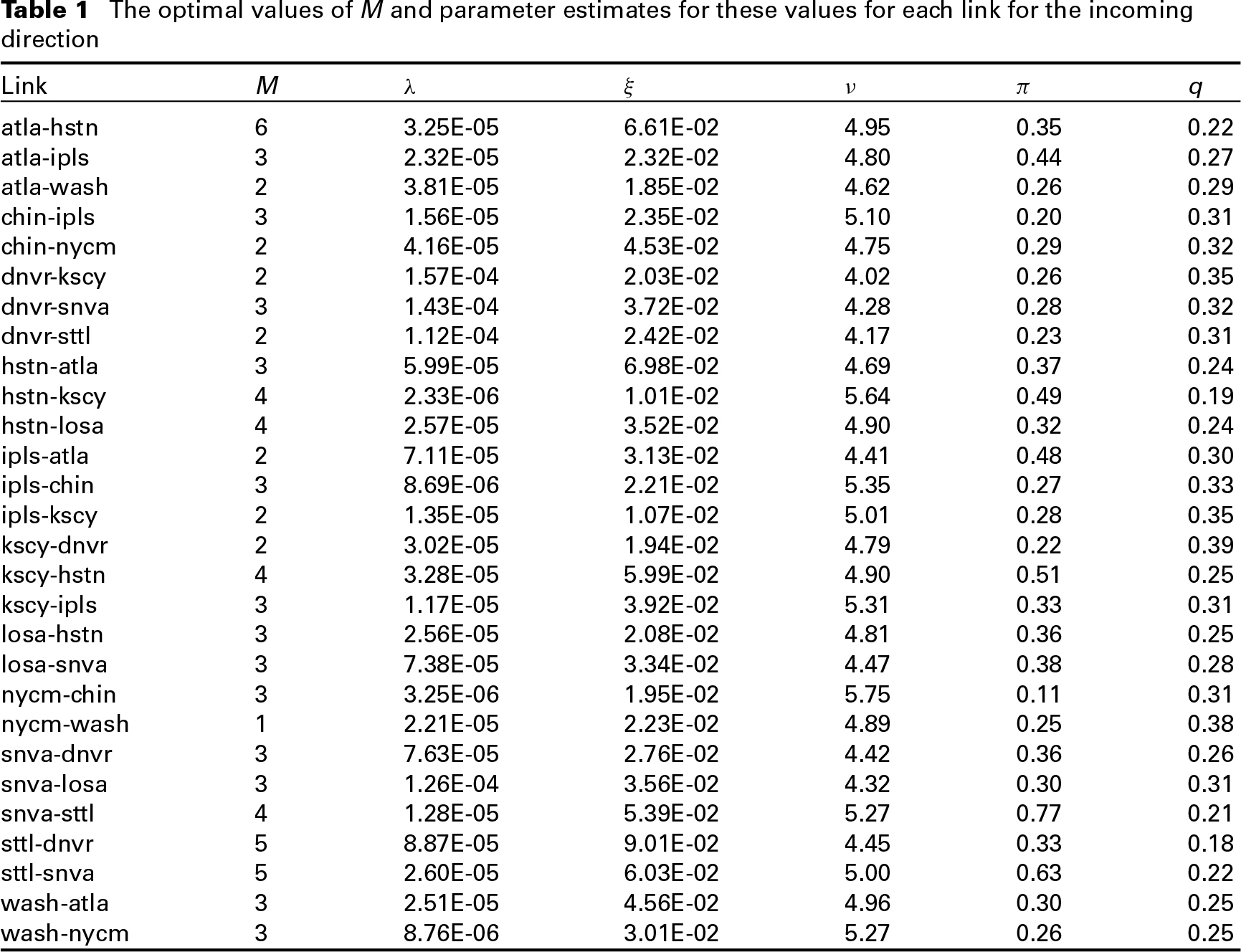
The optimal values of
We see that the parameter estimates are comparable across all links, so the selected statistical model appears to be appropriate; a misspecified model might work for some links, but not for others. Perhaps the most interesting finding is that the estimated values of
While the other parameters describe distributions, the value of
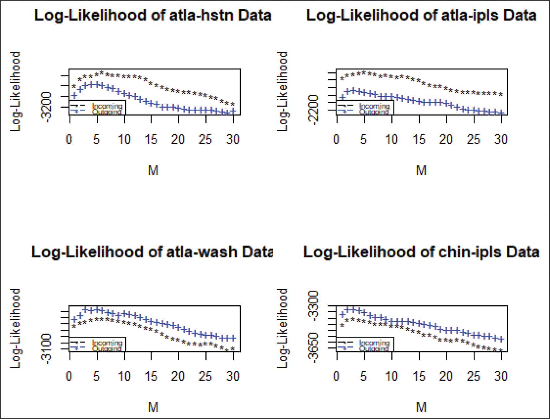
Plots of the log-likelihoods as a function of
for both the Atlanta
Houston link (left) and the Kansas City
Denver link (right). The log-likelihoods for the incoming and outgoing links are shown by ‘
’ and ‘
’ respectively. As one can see, the choice of
does not maximize the likelihood for any of the curves, and there appears to be a peak value for the likelihood in
for each
However, if we limit our information to that given merely by the interarrivals, and calculate the distribution of
Given that the model in this circumstance is a basic renewal process, calculating the likelihood function in theory is simple and can be written generally as
Table 2 gives evidence that our model indeed yields the higher likelihood with the same number of parameters. In addition, our model provides a better framework for taking into account both active and inactive periods separately, whereas in doing any further work along the lines of Kokoszka et al. (2020), we would need to define the distribution of the active periods conditional upon the length of the inter-arrivals, which is nontrivial. Thus, the model where we allow
An important application of a statistical model for the distribution of interarrival times in a renewal process is that it can be used to compute waiting times. Denote the current time by 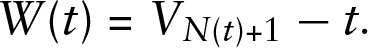
Somewhat counter-intuitively, the waiting time is stochastically larger than the interarrival time
Comparison of the maximum log-likelihoods computed in this article,
, with the maximum log-likelihoods computed using the model of Kokoszka et al. (2020),
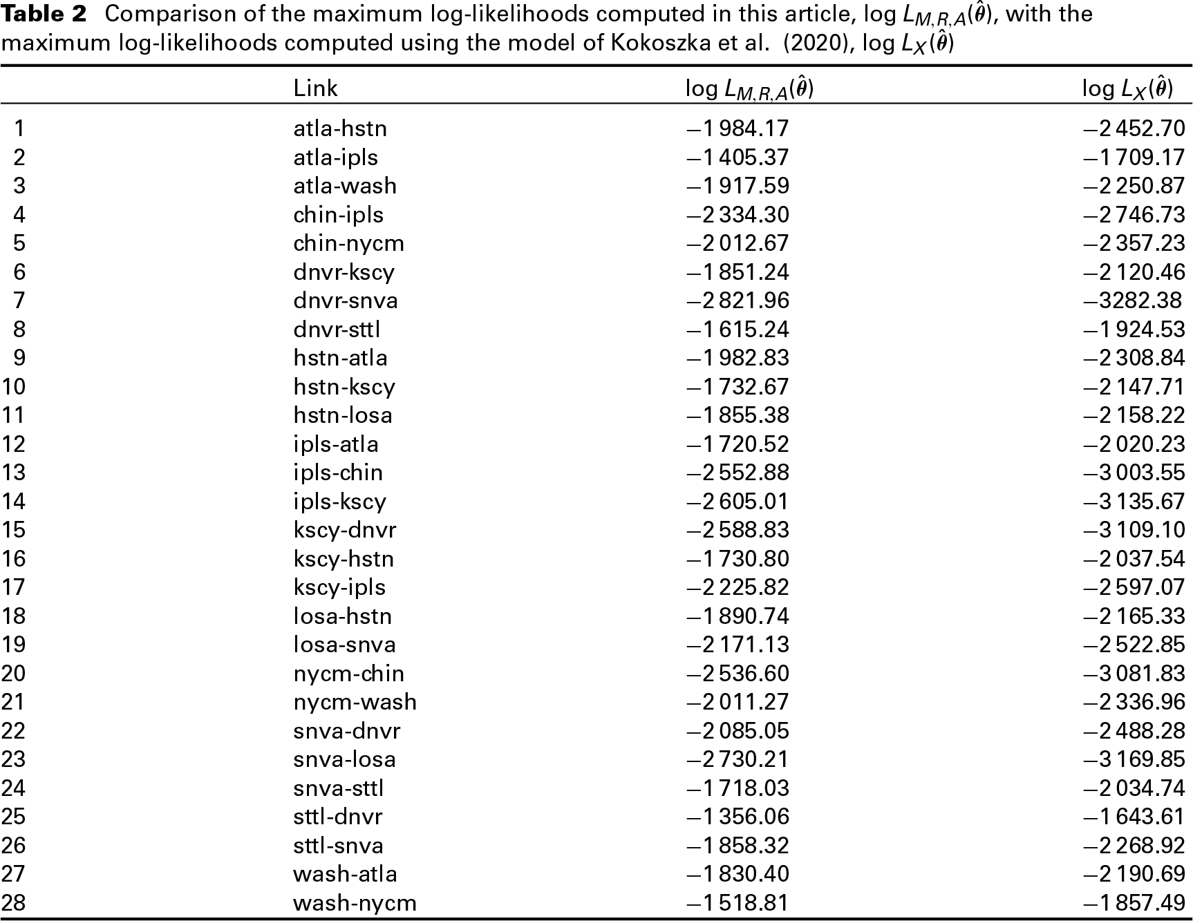
Comparison of the maximum log-likelihoods computed in this article,
Before comparing distributions derived from our model to those obtained by Kokoszka et al. (2020), we need to explain how the distribution of the waiting time can be computed, see Section 7.4.4 of Pinsky and Karlin (2011), or any other comprehensive textbook on renewal processes. Using the key renewal theorem, one can show that the equilibrium tail probabilities of 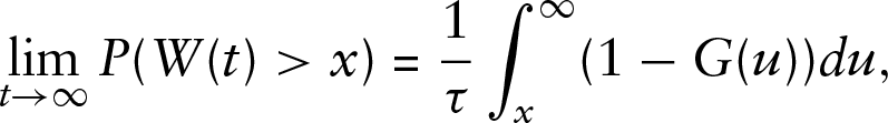
where

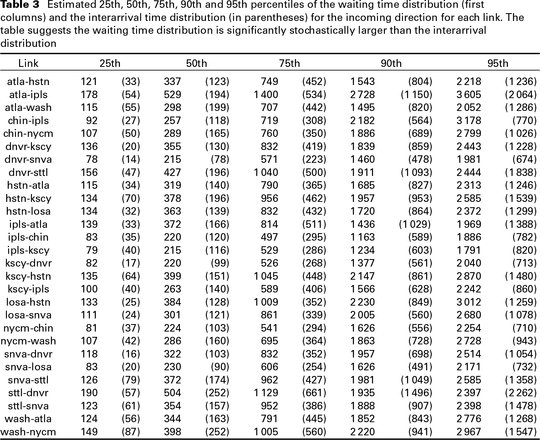
Estimated 25th, 50th, 75th, 90th and 95th percentiles of the waiting time distribution (first columns) and the interarrival time distribution (in parentheses) for the incoming direction for each link. The table suggests the waiting time distribution is significantly stochastically larger than the interarrival distribution
We note that the parameters 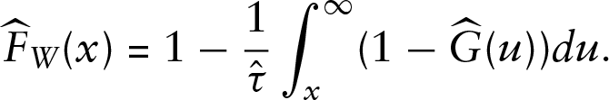
A central issue is to determine which estimators to use. Essentially the only consistent estimator of the cdf 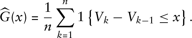
Recall that 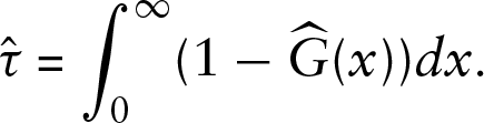
Using the above estimators, we computed the quantiles shown in Table 3. Note that since the interarrival lengths depend upon
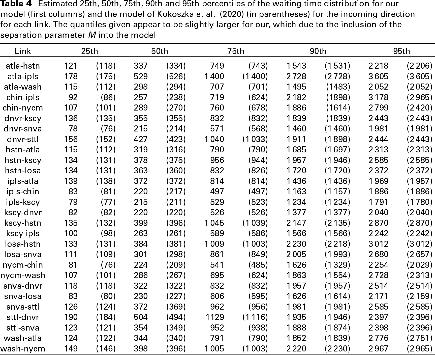
Table 4 compares the sample quantiles of the waiting time distribution for the model presented in this article and the model proposed by Kokoszka et al. (2020). The quantiles are slightly larger for our model. This can be explained by the introduction of the separation parameter of
A somewhat unexpected conclusion of the statistical model of Kokoszka et al. (2020) is that the expected waiting time for the arrival of the next anomaly is infinite. While infinite waiting times do occur in various stochastic models, their practical consequences are difficult to quantify and use. We now explain why the waiting time is infinite in the model of Kokoszka et al. (2020) and finite in our model. Denote by 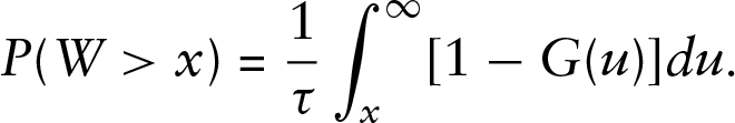
Denote by 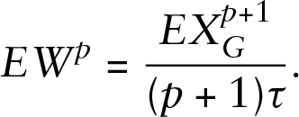
Estimated 25th, 50th, 75th, 90th and 95th percentiles of the waiting time distribution for our model (first columns) and the model of Kokoszka et al. (2020) (in parentheses) for the incoming direction for each link. The quantiles given appear to be slightly larger for our, which due to the inclusion of the separation parameter
If
We emphasize that the infinite waiting time following from the work Kokoszka et al. (2020) does not imply that its distribution will necessarily have larger quantiles than the distribution used in this article. To illustrate, if a positive random variable
Our work has focused on developing a statistical model for the propagation of internet anomalies in a US-wide network. The same model applies to all links, the parameters depend on the link. There are several novel elements in our approach that could potentially be useful in similar contexts. First, we showed how to conduct an exploratory analysis of an alternating renewal process to establish distributional and independence properties needed to construct a realistic statistical model. Second, we proposed nonstandard distributional models for the length of the inactive periods. Third, we proposed a regression approach to modelling the proportion of 1s as a response to the length of the active period. Fourth, we showed that the separation between the active periods,
A remaining question is how to describe the interaction between anomalies in various links. Through extensive experiments, we came to the conclusion that this would be very difficult within the framework considered in this article, and generally within a framework of statistical rather than engineering modelling. We now discuss the relevant issues and speculate on possible approaches.
Large hubs, the nodes of the network, play a significant role. Hardware and software placed at each node are designed to deal with anomalies. They never do it perfectly, so some anomalies, generally in a modified form, may travel to connecting links. What happens to an anomaly at a node depends on whether it is detected, and if so, how it is classified. A node can also be a source of an anomaly, for example, if a local network it serves is under attack or fails in some way. No such information is contained in our data. We speculate that due to such factors, there is no apparent connection between anomalous traffic at various links, as illustrated in Figure 11.
As the caption of Figure 11 emphasizes, and as has been noted earlier, for each unidirectional link, we actually have two datasets. This is because no measurements can be made in the link itself, which can be, for example, an optical fibre cable. Measurements are made by servers placed at certain locations in the hubs. Thus, say for an Atlanta
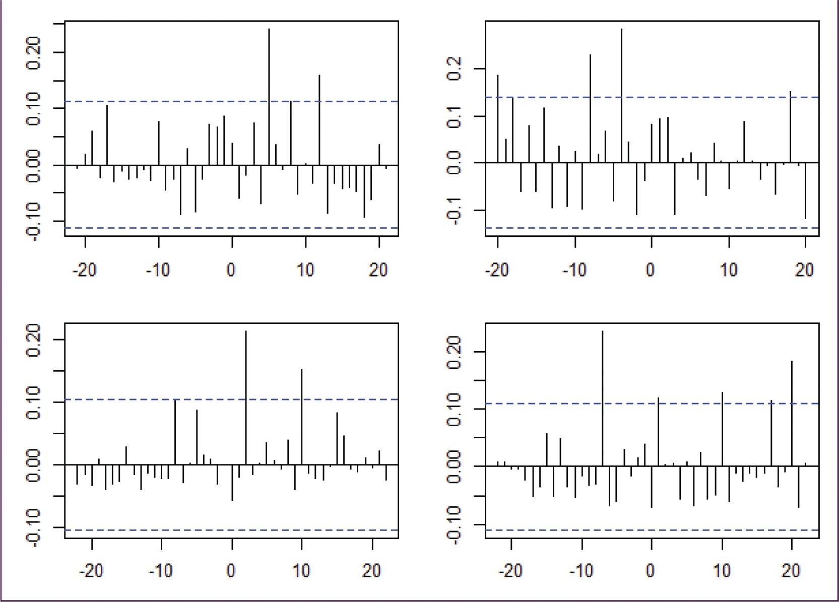
There is a statistical dependence between the incoming-outgoing pairs, as illustrated in Figure 12 The plots suggest that there may be significant correlation between the time series of the incoming-outgoing pairs. The lag structure of this correlation appears to be haphazard, we could not discern any pattern that would apply to all links.
The discussion above highlights the limits of modelling that can be done based on the available 0–1 strings. A more complete model would need to involve the action of the nodes and precise labelling of anomalies. The action at a note could potentially be described by an input–output model with multiple inputs and/or outputs. A model of this type for brain networks was recently proposed by Sienkiewicz et al. (2017), but it focuses on the node action, and there are no fixed links in the brain. A comprehensive hybrid engineering/statistical model would need to connect the statistical properties of anomalies propagation thorough the links to the action of the nodes. A much more comprehensive and detailed database would need to be constructed before advances in this direction can be made. The model developed in this article could be used to validate any future more comprehensive model, which would need to predict the properties we discovered and quantified.
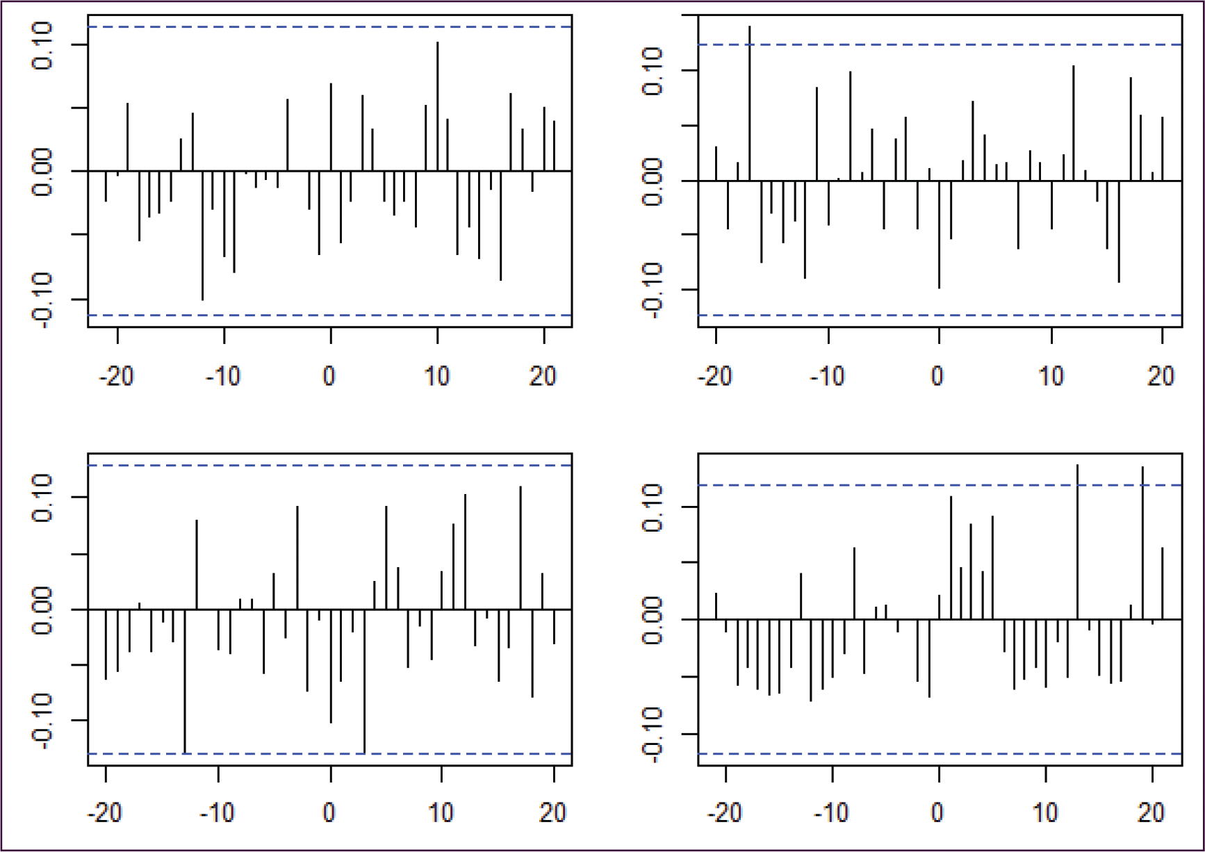
Cross-correlation plots for the interarrival times for the incoming Atlanta
Houston and Chicago
Indianapolis (top-left), incoming Denver
Sunnyvale and Indianapolis
Atlanta (top-right), outgoing Houston
Kansas City and Indianapolis
Atlanta (bottom-left), and outgoing Kansas City
Denver and Sunnyvale
Denver (bottom-right) links. These plots suggest no significant cross-correlation between these different links. From this, one would not expect that incoming and outgoing interarrivals corresponding to distinct links would not possess correlation
Finally, it would be of interest to investigate if the model remains valid, or how it would need to be modified, for anomalies extracted from internet traffic over a more recent time period. We hope that our research will motivate network engineers to construct a suitable database on which the model could be tested.
Cross-Correlation plots for the Atlanta
Houston, Atlanta
Indianapolis, Chicago
Indianapolis, and Denver
Sunnyvale incoming-outgoing pairs for
Footnotes
Acknowledgements
We thank Professor Anura P. Jayasumana of the CSU’s Department of Electrical and Computer Engineering for sharing the Internet2 anomalies data. We thank the Associate Editor and the referee for reading the article carefully and providing constructive criticism and advice, which helped us to improve the article.
Declaration of conflicting interests
The authors declared no potential conflicts of interest with respect to the research, authorship and/or publication of this article.
Funding
The authors disclosed receipt of the following financial support for the research, authorship and/or publication of this article: This research has been partially supported by NSF grants DMS 1737795 and DMS 1923142.