Discussion on: Shape constrained additive smooth models by Simon N. Wood

Abstract

1 Comment by Clara Bertinelli Salucci and Riccardo De Bin

We would like, first of all, to congratulate the author on this excellent article, which addresses the important topic of modelling and inference in the presence of inequality constraints. In our recent work at the interface of statistics and physics, we have realised how this setting arises naturally in many situations and therefore endorse the author’s opinion that constrained modelling really matter. As we saw in the article, the presence of constraints complicates the fitting procedures. Furthermore, special care is needed when making inference. When constraints restrict the parameter space, indeed, classical inferential tools no longer apply in their standard form, thus requiring a deeper investigation of the underlying asymptotic theory.

For example, consider the simple hypothesis test system

H_{0} : θ = 0 vs H_{1} : θ \neq 0

with $θ \in ℝ_{+}$ , that is, with θ scalar and constrained to have non-negative values. In this case, the likelihood ratio test statistic does not have the usual asymptotic $χ_{1}^{2}$ distribution, but a Chernoff distribution, namely a balanced mixture of a $χ_{0}^{2}$ and a $χ_{1}^{2}$ (Chernoff, 1954). This is due to the maximum likelihood estimator of the parameter being constrained to be non-negative: With probability 1/2, the unconstrained estimator would fall in the unallowed (negative) region and is therefore projected onto the boundary, yielding an estimate exactly equal to zero, while with probability 1/2 it lies in the interior and follows the usual asymptotic normal distribution.

1.1 Hypothesis testing

These constraint-induced distributional peculiarities of the test statistics based on large-sample theory seem relevant in the framework described in this article. As emphasised by the author, shape constraints on a smooth component $f_{j} (x_{j}) = \sum_{k = 1}^{K} β_{k} B_{m, k} (x_{j})$ , can be expressed as linear inequality constraints on the coefficient vector β. Under the null hypothesis f_j(x_j) = 0, these constraints place the parameter vector on the boundary of the parameter space.

Let us first consider constraints enforcing positivity: Imposing $f (x) \geq 0$ corresponds to $β_{j} \geq 0$ for all j, so under the null hypothesis for a vanishing smooth term, $H_{0} : β_{1} = \dots = β_{K} = 0$ , the K parameters are on the boundary. The likelihood ratio statistic converges to a mixture of chi-squared distributions with different degrees of freedom, namely ${\bar{χ}}^{2} = \sum_{k = 0}^{K} w_{k} χ_{k}^{2}$ , where, in this case, the weights w_k are determined by the intrinsic volumes of the cone of the alternative hypothesis (Shapiro, 1988; Takemura and Kuriki, 1997).

Consider the test statistics presented in Wood (2025, 3.3.3) and referred to in this article: Under the assumption that ${\hat{β}}_{j}$ has a Gaussian asymptotic distribution, the test statistic T, designed to account for the penalisation, is a weighted sum of $χ_{1}^{2}$ distributions. In the present case, however, the presence of constraints implies that the asymptotic distribution of ${\hat{β}}_{j}$ is no longer Gaussian, resulting in a test statistic that may instead converge to a more complicated weighted sum of mixtures of χ² distributions with different degrees of freedom. In other words, we suspect that, in the current framework involving constraints, the distribution of the test statistic is affected not only by the penalties but also by the constraints.

Similar considerations hold in the case of monotonicity and convexity constraints. Monotone increase can be imposed via $β_{1} \leq β_{2} \leq \dots \leq β_{K}$ . Equivalently, one can reparametrise in terms of an unconstrained intercept α = β₁ and nonnegative first differences γ_k ≥ 0. Testing f_j ≡ 0 corresponds to α = 0 and γ_k = 0, so that one parameter $(α \in ℝ)$ lies in the interior of the alternative space, while the remaining K − 1 parameters are on the boundary. As a result, the unpenalised version of the test statistic converges to a chi-squared mixture supported on $χ_{1}^{2}, \dots, χ_{K}^{2}$ . Convexity $f^{″} (x) \geq 0$ can be imposed similarly as nonnegativity constraints on suitable second differences of the spline coefficients. In this case, two parameters (an intercept and a linear trend) remain unconstrained, while the remaining coefficients are constrained to be nonnegative; consequently, the asymptotic chi-squared mixture is supported on $χ_{2}^{2}, \dots, χ_{K}^{2}$ .

Bootstrap-based testing offers an alternative to asymptotic hypothesis testing. As in the asymptotic setting, however, the presence of parameter constraints must be accounted for, requiring tools specifically designed for boundary problems (Cavaliere et al., 2017).

1.2 Confidence intervals

The issues discussed above are not limited to hypothesis testing, but also have important implications for the construction and interpretation of confidence intervals: When parameters are subject to inequality constraints, standard Wald-type confidence intervals based on asymptotic normality may exhibit poor coverage properties, particularly when the true parameter lies on or near the boundary of the parameter space. This point is clearly acknowledged by the author, who notes that parts of the parameter space may be effectively excluded by confidence intervals derived under regular asymptotic assumptions. Such behaviour is a direct consequence of the nonstandard asymptotic distribution of constrained estimators, which typically involves mixtures of truncated or degenerate distributions rather than a neat Gaussian limit. A natural question is whether a more explicit characterization of the asymptotic distribution of the estimators under the relevant boundary regimes could be exploited to construct confidence intervals with improved coverage. In principle, confidence sets derived from the appropriate mixture distributions, analogous to those arising in likelihood ratio testing, may provide a theoretically grounded result. However, their practical implementation in this specific framework might be challenging.

As well presented in the article, an alternative is represented once again by bootstrap methods. It is important to stress that the procedure considered by the author is not a plain implementation of standard bootstrap schemes, which have been shown to be first-order inconsistent in the presence of inequality constraints (Andrews, 2000). In this context, the author’s choice to resample score contributions rather than the constrained estimator itself is a well-justified strategy that avoids boundary-induced inconsistency issues. Andrews (2000) also discusses alternative approaches, such as subsampling and suitably modified bootstrap schemes, which may yield pointwise asymptotically valid inference in specific settings. These methods aim to approximate the nonstandard boundary asymptotic behaviour of the estimator, while the approach adopted in this article relies on a local Gaussian approximation and is then supplemented by an explicit bias correction.

1.3 Final remark

As a final remark, we would like to mention that the interaction between penalties and constraints may lead to interesting results. As an alternative to model selection through hypothesis testing, Nielsen and Rahbek (2024) showed that a sparsity-inducing penalisation such as smoothly clipped absolute deviation (SCAD), by forcing the zero coefficients to be exactly zero, leads the remaining coefficient estimators to have the usual Gaussian asymptotic distribution and retain $\sqrt{n}$ consistency. However, this result holds conditional on the selected model. Inference that subsequently treats the model as fixed, reducing the problem to an unconstrained setting, ignores selection uncertainty and potentially leads to anti-conservative tests and overly narrow confidence intervals.

2 Comment by Rosa M. Crujeiras

I would like to begin by sincerely thanking Simon Wood for this outstanding and generous contribution. Shape Constrained Additive Smooth Models is a technically rigorous, conceptually elegant and highly practical article that brings much-needed coherence to a topic of long-standing importance in applied statistical modelling. The article addresses a fundamental limitation of unconstrained smooth additive models: While flexible smooths are powerful, they can easily produce estimates that are scientifically implausible or difficult to interpret. By embedding shape constraints—such as monotonicity, convexity or positivity—directly into penalized spline representations, the author provides a unified framework in which prior scientific knowledge can be incorporated without sacrificing model flexibility or computational stability. Importantly, the framework allows constrained and unconstrained smooth terms to coexist within the same model.

A central strength of the article lies in its computational strategy. By expressing shape constraints as linear restrictions on spline coefficients, the author establishes a clear and elegant connection between smooth additive modelling and classical linear and quadratic programming. Apart from the computational part and the nice connection with quadratic and linear programming, I have been particularly interested in the inference proposals under shape constraints, which must obviously be handled with appropriate caution. My comments will focus primarily on this aspect.

As the author indicates, for interval estimation, treating constraints as fixed lead to under-coverage, whereas ignoring constraints (basing intervals on the unconstrained covariance matrix) lead to over-coverage, two issues that can be intuitively understood. In what follows, I would like to point out some issues for further research on this framework.

Formal treatment of the sampling variability of the active set. Section 5.1 correctly diagnoses the core difficulty: Treating the active set as fixed leads to severe under-coverage, because it ignores the fact that which constraints are binding is itself a random quantity depending on the data. Ignoring the constraints altogether leads to over-coverage. The bootstrap navigates between these extremes implicitly—each replicate may converge to a different active set—but without any theoretical guarantee. What is missing is an asymptotic distributional theory for $\hat{β}$ under active inequality constraints in the penalized spline setting. My guess is that this issue connects to the literature on cone testing for parametric regression (see Silvapulle and Sen, 2005), but I recognize that extending this theory to the nonparametric setting with estimated smoothing parameters is a genuinely hard open problem. Simon implicitly acknowledges this by offering the bootstrap as a pragmatic solution.

The bootstrap approach. The proposed approach in Section 5.2 is a bootstrap, corrected for smoothing bias using the scalar adjustment δ_j derived from the difference between the Bayesian and frequentist covariance matrices—a strategy rooted in Nychka (1988). On average across all scenarios and sample sizes the method achieves nominal 0.95 coverage, compared to 0.965 for intervals that ignore the constraints entirely. However, the simulation results in Figure 5 of the original article by Wood reveal that this average masks substantial over-coverage and slow convergence specifically in the location–scale models (Gaussian and Gamma). The correction δ_j is computed without accounting for the constraints, so it captures the smoothing bias as if the estimation were unconstrained. When the active set varies across bootstrap replicates—sometimes a constraint is binding, sometimes not—the effective smoothing bias changes in nature and a single scalar correction cannot adequately track it.

Scalability to large data and large models. Mentioned briefly in the conclusions, we may elaborate a bit more on this issue. The active-set quadratic programming algorithm is $O (p^{3})$ per iteration in the worst case, where p is the total number of basis coefficients. For rich distributional regression models with many smooth terms across multiple parameters, p can reach into the thousands. Similarly, the bootstrap requires re-fitting the full constrained model for each replicate, which compounds the computational burden. Integration with scalable methods—sparse QP solvers, stochastic gradient approaches or distributed Laplace approximations—may be identified as a direction for future work.

A view from functional data analysis (FDA). Viewing the smooth components in Wood’s framework as functional data objects offers a theoretically appealing avenue for confidence interval construction, though it comes with non-trivial limitations that temper its immediate practical promise. On the positive side, treating each estimated smooth f_j as a realization of a Gaussian process—with mean and covariance kernel $K_{j} (x, x^{'}) = B_{j} {(x)}^{T} V_{β} B_{j} (x)$ derived directly from the penalized likelihood, where B_j are the spline basis functions and V_β is the posterior covariance matrix—opens the door to simultaneous confidence bands based on the supremum distribution of the standardized process, which have a cleaner interpretation than the pointwise bootstrap bands currently proposed and are naturally compatible with asking whether a shape constraint holds globally rather than marginally at each point. The reproducing kernel Hilbert space (RKHS) structure induced by the smoothing penalty strengthens this connection further: the penalty β^TS_λβ defines an inner product on the space of smooth functions, making the space of admissible smooth components a well-defined RKHS whose geometry is entirely determined by the kernel associated with S_λ. This RKHS structure is precisely what FDA exploits and it means that the posterior covariance kernel K_j already encodes the metric geometry of the function space in a way that is compatible with FDA’s theoretical apparatus—including functional principal component decompositions and Karhunen–Loève expansions of the posterior process. The latter is particularly relevant: Expressing the posterior uncertainty in f_j through its leading functional principal components would provide a low-dimensional characterization of the dominant directions of estimation uncertainty, which could then be used to construct confidence bands that are both simultaneously valid and geometrically interpretable in terms of the shapes most likely to be confused with the estimate. However, on the negative side, several features of Wood’s setup create a genuine mismatch with standard FDA theory that should not be underestimated. First, the smooth components live in finite-rank spline spaces of fixed dimension rather than true infinite-dimensional function spaces, which means that the Gaussian process interpretation is exact only within this finite-dimensional approximation. Second, while the RKHS geometry is well-defined, the kernel K_j depends on the estimated smoothing parameters which are themselves random quantities whose uncertainty is not propagated into the covariance structure under Wood’s empirical Bayes treatment; this is a well-known limitation of plug-in posterior inference in Gaussian process regression and it means that the simultaneous bands derived from the plug-in kernel will undercover in finite samples to a degree that worsens as the effective degrees of freedom of the smooth decreases. Third, the projection of Gaussian process credible regions onto constraint cones in function space, while geometrically well-motivated, is computationally demanding in the general linear constraint setting, particularly for tensor product smooths where the constraint cone is defined by a large number of inequality constraints on a high-dimensional coefficient vector and no efficient algorithm for this projection currently exists in the penalized spline literature. Finally, shape-constrained FDA remains a comparatively underdeveloped area, with most existing theoretical results restricted to simple univariate monotonicity rather than the general framework—covering tensor product smooths, constraints on multiple derivative orders and parameters of distributional regression models—that Wood’s article requires, so that the theoretical guarantees available from FDA would need substantial extension before they could be applied with confidence to Wood’s framework. The FDA perspective and particularly the RKHS geometry and simultaneous band construction, is therefore best understood at this stage as a source of rich geometric intuition and a promising long-run theoretical scaffolding for improving constrained interval construction, rather than an immediately deployable solution—but one whose foundational compatibility with Wood’s framework makes it a natural and potentially fruitful direction, especially as the literature on shape-constrained inference in function spaces continues to mature.

In closing, I would like to thank Simon Wood once again for this impressive and thoughtfully crafted article that will be for sure a substantial contribution to both the methodology and practice of additive modelling. I am grateful for the opportunity to engage with such clear, rigorous and impactful work.

3 Comment by Maria Durbán

I enjoyed reading this article and was pleased to be invited to comment on it. Simon Wood offers a clear and thought-provoking discussion of shape constraints in models with additive smooth components, bringing together a range of ideas that are often treated separately in practice. In particular, the article provides a useful perspective on how constraints such as monotonicity or convexity can be expressed and handled within the GAM framework, and on the computational tools needed to fit such models reliably.

In my comments, I take up some of these ideas from a slightly different angle, focusing on an optimization-based view of shape-constrained smoothing that is closely related to the cone-based formulations discussed in the article. Rather than presenting an alternative to Simon’s approach, the aim is to highlight how similar geometric ideas can be combined with explicit smoothness penalties to handle a wide class of constraints and to reflect on a few applied settings where constraint-based methods seem particularly natural. I close with some general remarks prompted by the article.

3.1 Shape-constrained generalized additive models via conic optimization

Simon discusses in his article the cone projection framework developed by Meyer (2013, 2018), in which shape constraints are enforced by projecting the data vector onto a convex cone defined by the desired restrictions. In this approach, the fitted function satisfies the shape constraints by construction and estimation can be interpreted geometrically as a projection onto the constraint set. A characteristic feature of this framework is that regularisation is induced entirely by the shape constraints themselves: No additional smoothness penalty is introduced and the estimator corresponds to the least-squares projection onto the constraint cone.

Here, we draw attention to a related approach that builds on Meyer’s framework while incorporating explicit smoothness regularisation. Recent work by Navarro-García et al. (2023, 2024) proposes an optimization-based framework for shape-constrained generalized additive models that retains the geometric interpretation of shape constraints as convex restrictions, but embeds them within a penalised spline formulation. This allows shape and smoothness to be handled separately within a single convex optimization problem.

As in standard P-spline methodology, the unknown regression function is represented as a linear combination of B-spline basis functions and estimated by minimising a penalised least squares criterion, with smoothness controlled through a quadratic penalty on the spline coefficients. Shape constraints such as non-negativity, monotonicity and curvature are imposed by exploiting the fact that the fitted spline is a piecewise polynomial. On each knot interval, the spline can be rewritten explicitly as a low-degree polynomial whose coefficients depend linearly on the B-spline coefficients. This representation allows one to rely on a characterization of non-negative polynomials due to Bertsimas and Popescu (2002), yielding necessary and sufficient conditions for enforcing shape constraints in a convex, characterization-based form.

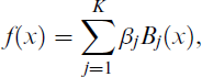
Let $y = {(y_{1}, \dots, y_{n})}^{⊤}$ denote the response vector and let X be the spline design matrix associated with a B-spline basis ${\{B_{j}\}}_{j = 1}^{K}$ . A smooth component is represented as

f (x) = \sum_{j = 1}^{K} β_{j} B_{j} (x),

with coefficient vector $β \in ℝ^{K}$ .

For cubic B-splines, the fitted function f is a continuous piecewise cubic polynomial. On each knot interval $[t_{q}, t_{q + 1}), f$ can be written explicitly as

f (x) = α_{q} x^{3} + β_{q} x^{2} + γ_{q} x + δ_{q}, x \in [t_{q}, t_{q + 1}),

with the coefficients (α_q, β_q, γ_q, δ_q) depending linearly on the spline coefficients β.

The shape constraints are then imposed directly on these local polynomial pieces. For a given interval q, the spline coefficients determine the corresponding polynomial and a pair of fixed matrices, A _q and B _q , are used to connect this polynomial to the chosen constraint. Roughly speaking, A _q extracts the polynomial coefficients coming from the spline, while B _q represents the same coefficients in the form required by the auxiliary matrix Z _q used to impose the constraint. Enforcing A _q (β) = B _q (Z _q ) simply ensures that the constraint is applied to the polynomial piece generated by the spline on that interval.

Putting these constraints together over all knot intervals and over the relevant covariate dimensions when needed, leads to a closed convex cone

C = \underset{q}{\cap} \{β \in ℝ^{K} : \exists Z_{q} \underline{≻} 0 such that A_{q} (β) = B_{q} (Z_{q})\} .

In other words, $C$ is the convex cone of spline coefficients β that give rise to functions satisfying the desired shape restrictions everywhere.

The framework extends naturally to generalized additive models by replacing the least squares term with a convex negative log-likelihood and to multivariate smooth functions through tensor-product spline bases. In these cases, the cone $C$ is defined as the intersection of cones corresponding to shape constraints imposed along selected covariate dimensions, allowing, for example, monotonicity in one variable and curvature constraints in another.

A possible limitation of this approach is that smoothing parameters are chosen based on the unconstrained fit. In practice, this does not seem to have a major impact in my experience, but it would be interesting to hear Simon’s perspective on this issue.

3.2 Final comments

Reading the article also brings to mind a few other applied settings where constraint-based ideas seem particularly helpful. One example is forecasting, and especially mortality forecasting. In this case, one often works with several age-specific or cohort-specific curves over time and extrapolations based on unconstrained smoothers can sometimes lead to awkward behaviour, such as mortality curves crossing in the future. Introducing shape constraints directly into the modelling step offers a simple way of avoiding these issues, rather than fixing them after the fact and helps to keep forecasts coherent across ages and time horizons. This seems particularly relevant when forecasts are used for planning or policy and it would be interesting to see how Simon’s approach deals with such constraints in a forecasting context.

Another area where similar ideas come up naturally is the estimation of production functions. These describe how inputs such as labour and capital combine to produce output. In particular, the function relating the inputs and the outputs has to be non-decreasing, concave and such that it envelops the decision-making units. Here, in principle, the constraints should not applied to individual smooth components, but to their combined effect, which raises the question of how this type of joint restriction could be handled within Simon’s framework.

4 Comment by Irène Gijbels

The author is to be congratulated for this very nice article on additive smooth modelling where the components possibly satisfy some shape constraints. It was with great pleasure that I read this excellent work. When using spline basis approximation, imposing the shape constraints leads to linear programming problems, while fitting the additive model results into sequential quadratic programming. I first formulate some general comments and then in following subsections discuss some more specific research issues.

The article starts with a nice set of examples showing a diversity of shape constraint issues in applications. The examples also reveal several open questions. When in a preliminary stage a model has been selected, this likely is done under unconstrained estimation. This brings up the question whether constrained estimation is not preferably also in a preliminary model selection step. A related question is whether model selection and estimation steps should not be done simultaneously. Further, what to be done if a curve seems to exhibit some clearly different shapes in distinct regions. For example a curve can be flat (no influence of the covariate) in a subdomain (region), but having a clear non-linear behaviour outside that region.

When using B-spline basis expansions for a smooth function and imposing the shape constraint via a linear (in) equality on the coefficients, the estimator satisfies the constraint only in a finite set of values. However, depending on the degree of the B-spline and the imposed constraint the validity of the constraint may hold in whole the domain. Consider a B-spline basis with K + 1 equispaced knot points (denoted ξ₀, · · ·, ξ_K) and let q denote the degree of the basis functions. Denoting the basis functions by b_j(·; q), for $j = 1, \dots, \tilde{m} (with \tilde{m} = K + q)$ , a B-spline expansion for a function f is $f (t) = \sum_{j = 1}^{\tilde{m}} γ_{j} b_{j} (t; q)$ interval defined by the smallest and largest knot points, are as follows.

For a quadratic spline, monotonicity in the knot points ξ₀, · · ·, ξ_K is equivalent to monotonicity on the whole domain [ξ₀, ξ_K].

For a cubic spline, convexity in the knot points ξ₀, · · ·, ξ_K is equivalent to convexity on the whole domain [ξ₀, ξ_K].

See Ahkim et al. (2017) and in particular Lemma 2 therein.

To be noted is also that when the constraint is formulated in terms of a linear functional, the proposed approach is to use a discrete approximation to the functional. The accuracy of such a discrete approximation depends on choices of some parameters and this impacts also how general (in the domain) the imposed constraint is satisfied.

4.1 Shape constraints and interaction terms

If additive models are dictated to include interaction terms, shape constrained estimation becomes a more tricky issue. The author mentions that a simple re-parametrization approach may be not possible if constraints are required on more than one marginal. Avoiding constraint redundancy can be part of a solution here and how this is to be avoided is explained when a positivity constraint is imposed on two margins. An interaction term however may exhibit the possible behaviour that in different components (margins) different type of constraints (should) hold. An example is a bivariate function f(x, y) for which the function $x \mapsto f (x, y)$ is monotone for each y and the function $y \mapsto f (x, y)$ is convex for each x. It would be interesting to discuss approaches that would allow different shape constraints for the separate components in a higher-degree interaction term.

4.2 Varying coefficient models and shape constraints

In case of longitudinal data, the response variable y and the covariates (x₁, · · ·, x_d), may evolve over (say) time t and for each subject i in the study, observations of y(t) and (x₁(t), · · ·, x_d(t)) may be available on different time points, denoted $t_{i 1}, \dots, t_{i n_{i}}$ with n_i denoting the number of measurements (time points). For subject i, the measurements of response and covariates at time point t_ij are then denoted as (t_ij, y(t_ij), x₁(t_ij), · · ·, x_d(t_ij). A varying coefficient model can take the form

y (t_{i j}) = β_{0} (t_{i j}) + \sum_{p = 1}^{d} β_{p} (t_{i j}) x_{p} (t_{i j}) + ε (t_{i j}),

where $β_{0}, \dots, β_{d}$ denote the unknown univariate varying coefficient functions and ε(t_ij) is a stochastic error term. Obviously there could be reasons for having interaction terms between two (or more) covariates into the modelling. Note that a constant function β_p(·) would mean that the effect of the covariate x_p would be constant over time. A monotonically increasing (positive) function β_p(·) indicates that the effect of the covariate on the response increases over time. See for example Ahkim et al. (2017) for testing procedures for testing for monotonicity or convexity of the varying coefficients, modelled via B-spline approximation.

The use of varying coefficient models goes beyond the study of longitudinal data (where the dynamics is on a time scale). Indeed, this kind of model has been used extensively to describe dynamic effects of one (or more) variables on other variables in various scientific areas. See, for example, Fan and Zhang (2008) and references therein and recent articles such as Delgado and Arteaga-Molina (2021), and Yang et al. (2023). In the latter article, containing an application in a medical context, the interest is also in finding regions with zero-effects and a smooth effect outside these regions.

The use of varying coefficient models also goes beyond the interest of investigating the conditional mean. Indeed, conditional quantile regression is of particular interest in medical studies, where the startup of a medical treatment, might depend on the distributional response exceeding a certain threshold. See, for example, Andriyana et al. (2014). Particular challenges in quantile regression for longitudinal data (or beyond), are the non-crossing of quantile curves or homoscedasticity versus heteroscedasticity. A homoscedasticity setting can be translated into constancy of a (unknown) variability function (that also can be modelled using B-spline approximation). See Andriyana et al. (2018).

It would be interesting to see to which extent the presented framework can deal with these research items.

4.3 Shape constrained additive smooth models and beyond

The article focuses on additive models with smooth component functions. The order q of the B-spline representation seems to be taken the same for each univariate function or for each component in a tensor product setting. In applications though the component functions can show different degrees of smoothness and even might not be smooth. Effects of covariates might be linear or highly non-linear or piecewise linear (non-differentiable functions) or even presented by a discontinuous function (for example different constant effects in different regions). This raises the question to what extent the overall framework presented by the author can be extended to accommodate components in the additive model that exhibit various degrees of smoothness or even non-smooth and smooth components. Partial answers for the first issue might be to consider B-splines of various degrees, as well as different penalty functions.

5 Comment by Thomas Kneib

Reading articles by Simon Wood is always a great enjoyment and an excellent opportunity to acquire new insights alike. It has therefore been a pleasure to be asked to contribute to the discussion of this article, focussing on shape constraints (such as monotonicity or convexity constraints) applicable in a wide range of models comprising additive predictors composed of smooth functions. It turns out that linear (in)equality constraints on the coefficients of a basis expansion yield a very general class of constraints and Simon offers insights into the construction and handling of such constraints as well as appropriate fitting methods including the determination of the smoothing parameter. In the following, I will discuss an alternative approach for achieving constraints based on an additional penalty term and a possible extension of Simon’s framework to the consideration of orthogonality constraints which can also be expressed as linear equality constraints on basis coefficients of smooth terms.

5.1 Constraints based on extra penalties

As noted in Simon’s article, a monotonically increasing sequence of B-spline basis coefficients $β_{1} \leq β_{2} \leq \dots \leq β_{J}$ is sufficient for ensuring a monotonically increasing effect estimate. This naturally translates into J − 1 linear inequality constraints of the form $β_{j} - β_{j - 1} \geq 0, j = 2, \dots, J$ which can be directly incorporated into the fitting procedure as outlined by Simon.

An alternative approach that may be easier to augment to existing implementations can be based on an additional penalty term that encourages the linear inequality constraints. More precisely, consider a penalty term based on asymmetric differences defined as

λ \sum_{j = 1}^{J} v_{j} {(β_{j} - β_{j - 1})}^{2} = λ β^{⊤} D^{⊤} V D β

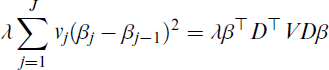
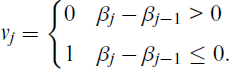
where D is a first order difference matrix and V = diag(v₂, …, v_J) is a diagonal weight matrix with entries

v_{j} = \{\begin{matrix} 0 β_{j} - β_{j - 1} > 0 \\ 1 β_{j} - β_{j - 1} \leq 0. \end{matrix}

Adding this penalty term (additionally to the usual smoothness penalty) to the optimization criterion of interest will then encourage the monotonicity constraint, if a large penalty parameter λ is assigned to the asymmetric differences. Fitting the model in an iterative procedure such as Fisher scoring will then include updating the definition of the weights v_j such that the penalty for the constraint only becomes effective when needed and will leave the estimate unchanged otherwise.

While being conceptually simple, this approach of course comes with the disadvantage that the constraint is not strictly ensured, but only encouraged by the penalty. The level of encouragement depends on the value of the penalty parameter assigned to the penalty for the constraint. Still, the extra penalty approach can be effectively used not only for monotonicity constraints, but also for a variety of other constraints. This has first been noted by Eilers (2005) and Bollaerts et al. (2006) and has later been put into a unified framework by Hofner et al. (2016). For example, using a similar type of weights as above applied to second order differences allows to include concavity and convexity constraints. One can also formulate boundary constraints for constant or linear extrapolations beyond the range of observed covariate values or define constraints for tensor product smooths. While the framework presented in Hofner et al. (2016) is based on functional gradient descent boosting, it can readily be used in penalized maximum likelihood frameworks as well.

5.2 Constraints based on orthogonality in function spaces

While Simon’s article focusses on shape constraints, the framework of linear constraints can also be natively used for orthogonality constraints. For example, to render additive models identifiable, one is often interested in making all function estimates orthogonal to a constant effect, but one may similarly be interested to make the estimates orthogonal to linear effects or to remove main effects from a tensor product interactions.

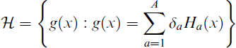
As shown in ?, such constraints also fit into the framework of linear constraints. The main idea is to define the constraints based on a space of functions

H = \{g (x) : g (x) = \sum_{a = 1}^{A} δ_{a} H_{a} (x)\}

that defines the type of functions the effect of interest f(x) should be orthogonal to. In this formulation, H_a(x), a = 1, …, A are a set of basis functions generating the function space $H$ , for example a constant and a linear function in x if f(x) should be made orthogonal to a linear effect.

The linear constraints are then derived from assuming orthogonality of any basis function B_j(x) involved in the definition of the effect f(x) to any basis function of the constraint space H_a(x), i.e.

\int f (x) H_{a} (x) d x = \sum_{j = 1}^{J} β_{j} \int B_{j} (x) H_{a} (x) d x = 0, a = 1, \dots, A .

This leads to the constraint matrix

L [a, j] = \int B_{j} (x) H_{a} (x) d x, a = 1, \dots, A, j = 1, \dots, J,

which can directly be fed into Simon’s optimization procedures.

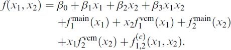
As discussed in ?, this construction is widely applicable to ensure identifiability in additive models and to facilitate interpretation by decomposing complex effects such as tensor product smooths into simpler components. For example, a bivariate tensor product interaction f(x₁, x₂) can be orthogonally decomposed into linear main effects β₁x₁, β₂x₂ and a linear interaction effect β₃x₁x₂, nonlinear main effects $f_{1}^{main} (x_{1}), f_{2}^{main} (x_{2})$ , varying coefficient terms $x_{2} f_{1}^{v c m} (x_{1}), x_{1} f_{2}^{v c m} (x_{2})$ and a remaining interaction term $f_{1, 2}^{(c)} (x_{1}, x_{2})$ yielding the representation

\begin{matrix} f (x_{1}, x_{2}) = β_{0} + β_{1} x_{1} + β_{2} x_{2} + β_{3} x_{1} x_{2} \\ + f_{1}^{main} (x_{1}) + x_{2} f_{1}^{v c m} (x_{1}) + f_{2}^{main} (x_{2}) \\ + x_{1} f_{2}^{v c m} (x_{2}) + f_{1, 2}^{(c)} (x_{1}, x_{2}) . \end{matrix}

All these effects are, by construction, intermingled in the tensor product interaction and are then also assigned a single smoothness parameter. The orthogonal decomposition yields nicely interpretable effects and also provides additional flexibility by allowing for separate smoothness parameters for all nonlinear effects. While the work in ? relies on Bayesian inference based on Markov chain Monte Carlo simulations, where the constraints are ensured during the sampling process, the work by Simon makes orthogonality constraints also accessible in penalized likelihood settings.

5.3 Closing remarks

Finally, I would like to briefly touch a general issue related to the incorporation of constraints into model fitting. While I completely concur with Simon’s presentation, an alternative view may be that violations of constraints that would be expected based on theoretical considerations could also be seen as indications of either model misspecification or problematic observations. The former might then call for modifications of the model, rather than the addition of constraints, while the latter may question the validity of the available sample for answering the scientific question of interest and I would be interested in learning about Simon’s thoughts on these aspects.

6 Comment by Nikolaus Umlauf

Reading Simon Wood’s article on shape-constrained additive smooth models was, as always, both enjoyable and stimulating. The article provides a remarkably clear and general framework for incorporating linear equality and inequality constraints into penalized spline-based additive models and demonstrates convincingly how quadratic programming combined with the extended Fellner–Schall method yields a practically usable solution. This contribution also connects to a broader literature on constrained regression and shape-constrained smoothing; see, for example, Hofner et al. (2016) and Meyer (2018). More generally, modern developments of generalized additive models increasingly extend beyond mean regression towards models for entire conditional distributions (Wood, 2025).

In this comment I would like to focus on a perspective that is only touched upon briefly but, in my view, deserves particular emphasis: The role of shape constraints in distributional regression models, such as generalized additive models for location, scale and shape (GAMLSS; Stasinopoulos and Rigby, 2007; Stasinopoulos et al., 2024) and related distributional regression approaches (Umlauf and Kneib, 2018; Kneib, 2013). While shape constraints are often motivated by interpretability in mean regression, their role in multi-parameter distributional models extends beyond interpretability and becomes structural.

This perspective is particularly natural in the context of distributional regression frameworks where multiple parameters of the response distribution are modeled as functions of covariates simultaneously. In such models, the interaction between smooth predictors across distributional parameters can strongly influence the implied distributional shape, making structural constraints on individual components or derived quantities potentially valuable (Umlauf et al., 2018; Kneib et al., 2019).

6.1 Constraints beyond the mean

In classical GAM settings, shape constraints are typically imposed on the conditional mean function, for example to enforce monotonicity or convexity based on theoretical knowledge. In distributional regression, however, several parameters of the response distribution are modeled simultaneously, for example

g_{1} (μ_{i}) = η_{1 i}, g_{2} (σ_{i}) = η_{2 i}, g_{3} (v_{i}) = η_{3 i}, \dots

where each predictor $η_{k i}$ may contain smooth components.

Within Simon’s framework, imposing shape constraints on these predictors is conceptually straightforward. Monotonicity or convexity can be enforced separately for smooth terms in the mean, scale or shape predictors by applying linear constraints to the corresponding coefficient vectors.

However, in such multi-parameter settings, unconstrained smooth terms for scale, skewness or tail parameters may produce distributional shapes that are mathematically admissible but scientifically implausible. Examples include: Decreasing variance where variability is expected to increase, highly oscillatory scale functions compensating for misspecification of the mean or also implausible tail behaviour induced by overly flexible shape parameters.

In these situations, constraints are not merely aesthetic refinements. Rather, they encode structural information about the data-generating mechanism and help prevent unrealistic distributional behaviour. This suggests that in distributional regression, shape constraints may be useful not only for improving interpretability of individual effects, but also for promoting coherent distributional behaviour.

6.2 Constraints and weak identifiability in multi-parameter models

A second point concerns the interaction between constraints and weak identifiability. In GAMLSS-type models, different distributional parameters may partially compensate each other. For example:

A decreasing mean combined with increasing variance may generate a similar likelihood as a flatter mean with smaller variance.

Shape parameters may absorb effects that could alternatively be captured by scale.

In hazard-based models, wiggliness in the baseline hazard may trade off against time-varying covariate effects.

Such phenomena do not necessarily imply formal non-identifiability, but they often lead to weakly identified models in finite samples. Penalization partially mitigates this issue by discouraging overly complex functions. However, smoothing penalties alone do not prevent certain structurally implausible combinations of effects.

Shape constraints can therefore act as structural regularizers, restricting the parameter space in ways that reduce confounding across distributional components. Examples include (a) enforcing monotonicity of a variance function, (b) imposing concavity on a mean effect where diminishing returns are expected or also (c) restricting curvature of tail parameters.

In this sense, constraints complement smoothing penalties: While penalties control local complexity, constraints restrict global behaviour and directionality. In multi-parameter models, this distinction can become particularly important.

6.3 Constraints on derived quantities

An additional subtlety arises from the fact that in distributional regression, smooth terms are not usually the quantities of primary interest. Instead, they influence derived quantities such as quantile functions, hazard functions, survival probabilities or also tail probabilities.

In contrast to separate quantile regressions, quantiles in distributional regression cannot cross for fixed covariate values, since they are derived from a single parametric distribution. Nevertheless, parameter-wise shape constraints do not necessarily imply corresponding shape properties of derived functionals.

To illustrate this point, consider a Gaussian model with

Y | x \sim N (μ (x), σ {(x)}^{2}),

so that the τ-quantile is

Q_{τ} (x) = μ (x) + z_{τ} σ (x),

where $z_{τ} = Φ^{- 1} (τ)$ is the τ-quantile of the standard normal distribution.

Differentiating with respect to x yields

\frac{d}{d x} Q_{τ} (x) = μ^{'} (x) + z_{τ} σ^{'} (x) .

Suppose that both μ(x) and σ(x) are increasing; that is, $μ^{'} (x) \geq 0$ and $σ^{'} (x) \geq 0$ . For upper quantiles with τ > 0.5, we have z_τ > 0 and hence both terms on the right-hand side are nonnegative, implying that Q_τ(x) is increasing.

However, for lower quantiles with τ < 0.5, we have z_τ < 0. In this case the term $z_{τ} σ^{'} (x)$ becomes nonpositive. If the increase in scale is sufficiently strong relative to the increase in location, the derivative of Q_τ(x) may become negative, despite both μ(x) and σ(x) being increasing.

This illustrates a more general phenomenon: Shape constraints imposed separately on distribution parameters do not generally propagate to derived distributional functionals. In many distributional regression models, structural properties such as monotonicity of quantile or hazard functions depend on interactions between several distributional parameters, rather than on the behaviour of individual predictors alone.

6.4 Cross-parameter constraints

Perhaps the most intriguing extension concerns constraints that involve multiple distributional parameters simultaneously. Many scientifically motivated restrictions are not separable across parameters. Examples include (a) shape restrictions on a fixed quantile curve, (b) monotonicity of a hazard function depending jointly on location and scale and (c) structural constraints ensuring unimodality or specific tail behaviour.

In particular, constraints on derived quantities such as quantiles or hazards typically induce nonlinear relationships between several coefficient vectors, which are not directly covered by the current linear constraint formulation. Such restrictions translate into joint constraints on several coefficient vectors, thereby coupling predictors across distributional parameters. In the current framework, constraints are typically imposed within a single smooth term. Extending this idea to cross-parameter constraints would require a joint formulation across multiple coefficient blocks.

From a computational perspective this would still lead to a constrained optimization problem, although the resulting constraints will in general no longer be linear in the coefficients. Conceptually, however, this shifts constraints from being local to a single effect toward representing global distributional restrictions.

Developing systematic approaches for incorporating such joint constraints within penalized likelihood frameworks for distributional regression could substantially expand the practical scope of shape-constrained modelling.

6.5 Concluding remarks

Simon Wood’s article provides a powerful and general computational foundation for shape-constrained additive modelling. From the perspective of distributional regression, constraints are not merely tools for improving interpretability. They can reduce weak identifiability between distributional components, stabilize estimation in multi-parameter settings and encode structural information about the implied distribution.

More broadly, the discussion above suggests that in distributional regression the most meaningful shape restrictions may not always act on individual model components, but on the implied distributional functionals themselves. Understanding how such constraints propagate through multi-parameter models and how they can be incorporated into computationally efficient estimation procedures appears to be a promising direction for future research.

7 Rejoinder by Simon N. Wood

Thanks to all the discussants for their substantial and thought provoking contributions. I can find little to disagree with in any of them. I particularly agree with Clara Bertinelli Salucci, Riccardo De Bin and Rosa Crujeiras that interval estimation and testing is the area most in need of improvement and where theory that really deals with the uncertainty in the active set represents the most interesting challenge. As Clara Bertinelli Salucci and Riccardo De Bin have noticed, the discussion of p-values in my article is cursory and the constraints considerably complicate the null distributions involved. In the software, I have actually computed p-values as if the model were unconstrained, but in the same way that this makes confidence intervals somewhat too wide, it is bound to result in suboptimal power. Rosa Crujeiras discusses a rich set of ideas for developing improved intervals, which I hope will persuade someone to rise to the challenge. The points about the scalar bias correction are of course correct, but it would be very interesting to see how big the effects are in reality. On scalability, it is worth noting that the bootstrap is perhaps slightly less costly than implied. Sequential QP estimation of the full model involves a number of O(np²) steps (where typically p = o(n¹ ^/ ³)) while each bootstrap replicated involves a single O(p³) step.

Maria Durbán’s trick for getting necessary and sufficient shape constraint conditions for splines is very nice. On the subject of joint constraints—any linear constraint on the parameters can be handled by the methods—but the software currently only implements term-wise constraints (out of laziness, rather than any fundamental problem).

I agree with Irène Gijbels that in many cases one would want to include shape constraints in the initial analysis up front, rather than following my introductory examples, in which this was only done after an initial unconstrained fit. But this has to be a case-by-case decision, as Thomas Kneib’s final comments emphasise: If we constrain, there is always the danger that we bludgeon the model into compliance with our pre-conceptions, in defiance of the data. So for every case, such as the COVID example or the examples discussed by Nikolas Umlauf, where the constraint is essential for sane inference, there are others where the shape constrained model really should be compared to its unconstrained equivalent. On simultaneous model selection and fitting, the framework does allow the inclusion of null space penalties for this purpose, but this is of course only one of the approaches that one might want to take to this issue. The comments on the interval over which the constraints hold are also important. Of course for B-splines we anyway need to explicitly modify the basis for sensible extrapolation outside the interval covered by the inner knots. With cubic B-splines we might simply insist on linear extrapolation from the function value and slope at the appropriate knots: Extending monotonicity constraints to the extrapolation is then easy. On interactions, the approach actually already allows different shape constraints on different directions of tensor product smooths of arbitrary dimension. The highlighting of shape constrained varying coefficient models is valuable, I think: Varying coefficient terms are examples of the general linear functionals of smooths covered by the framework and in software are specified using by variables. The challenges of crossing quantiles (estimated non-parametrically) are more difficult. On different orders of smoothness, the framework and software allows different orders of spline and penalty, with mixtures possible within interaction terms as well as between terms. Piecewise linear terms are also available, as are Gaussian Markov random fields which are piecewise constant. That said, there are many more types of term that could be implemented.

Thomas Kneib’s discussion of imposing constraints via penalties is particularly interesting with regard to alternative routes to better calibrated inference, discussed above and Nikolaus Umlauf’s discussion of constraints on derived quantities. Inference based on this approach requires a somewhat different starting point to that required by the active set or cone-projection methods and might provide an alternative route to better justified intervals, while non-linear constraints are more readily incorporated via penalties. The orthogonality constraints example with Smoothing-Spline-ANOVA type smooth interactions is very interesting, but I suspect that absorbing the resulting equality constraints upfront is probably preferable to directly using the methods covered in my article (without inequality constraints to worry about, the linear and quadratic programming machinery is probably overkill).

I found Nikolaus Umlauf’s comments about the role of constraints in distributional regression particularly illuminating. I had not thought about these issues before, but the notion of structural regularization in the face of weak identifiability or the structural encoding of essential features of the data gathering process seem rather important. The constraints on derived quantities problem is also a big challenge in this area: The article’s framework allows linear constraints linking different terms and different predictors, but many target derived quantities are indeed not on the linear predictor scale. Other interesting constraints even on single terms are also non-linear: For example the restriction that a smooth should be unimodal. Such non-linear constraints will perhaps inevitably lead back to the penalization approach discussed by Thomas Kneib. That said, my guess is that, when constraints are linear, an approach such as the one described in my article is likely to have some advantages in terms of stability and simplicity.

Footnotes

Declaration of Conflicting Interests

The authors declared no potential conflicts of interest with respect to the research, authorship and/or publication of this article.

Funding

The authors received no financial support for the research, authorship and/or publication of this article.

ORCID iDs

Clara Bertinelli Salucci

Rosa M. Crujeiras

Riccardo De Bin

Maria Durbán

Irène Gijbels

Thomas Kneib

Nikolaus Umlauf

Simon N. Wood

References

Ahkim

, Gijbels

, & Verhasselt

(2017). Shape testing in varying coefficient models. Test , 26(2), 429–450. doi:10.1007/s11749-0 16-0518-y.

Andrews

D. W.

(2000). Inconsistency of the boot-strap when a parameter is on the boundary of the parameter space. Econometrica , 68, 399–405

Andriyana

, Gijbels

, & Verhasselt

(2014). Shape testing in varying P-splines quantile regression estimation in varying co-efficient models. Test , 23, 153–194. doi:10.1 007/s11749-013-0346-2.

Andriyana

, Gijbels

, & Verhasselt

(2018). Quantile regression in varying co-efficient models: non-crossingness and het-eroscedasticity. Statistical Papers , 59(4), 1589–1621. doi:10.1007/s00362-016-0847-7.

Bertsimas

, & Popescu

(2002). On the re-lation between option and stock prices: A convex optimization approach. Operations Research , 50(2), 358–374. doi:10.1287/op re.50.2.358.424.

Bollaerts

, Eilers

P. H. C.

, & van Mechelen

(2006). Simple and multiple p-splines regres-sion with shape constraints. British Journal of Mathematical and Statistical Psychology , 59(2), 451–469. doi:https://doi.org/10.1348/ 000711005X84293.

Cavaliere

, Nielsen

H. B.

, & Rahbek

(2017). On the consistency of bootstrap test-ing for a parameter on the boundary of the parameter space. Journal of Time Series Analysis , 38, 513–534.

Chernoff

(1954). On the distribution of the like-lihood ratio. The Annals of Mathematical Statistics , 25, 573–578.

Delgado

M. A.

, & Arteaga-Molina

L. A.

(2021). Testing constancy in varying co-efficient models. Journal of Econometrics , 222(1), 625–644. doi:10.1016/j.jeconom.2020.07.041.

10.

Eilers

P. H. C.

(2005). Unimodal smoothing. Jour-nal of Chemometrics , 19(5-7), 317–328. doi:https://doi.org/10.1002/cem.935.

11.

Fan

, & Zhang

(2008). Statistical methods with varying coefficient models. Statistics and Its Interface , 1(1), 179–195. doi:10.431 0/SII.2008.v1.n1.a15.

12.

Hofner

, Kneib

, & Hothorn

(2016). A unified framework of constrained regression. Statistics and Computing , 26, 1–14.

13.

Kneib

(2013). Beyond mean regression. Statis-tical Modelling , 13(4), 275–303. doi:10.1177/ 1471082X13494159.

14.

Kneib

, Klein

, Lang

, & Umlauf

(2019). Modular regression - a Lego sys-tem for building structured additive dis-tributional regression models with tensor product interactions. Test , 28(1), 1–39. doi: 10.1007/s11749-019-00631-z.

15.

Meyer

M. C.

(2013). Semi-parametric additive constrained regression. Journal of Nonparametric Statistics , 25(3), 715–730. doi:10.1080/0485252.2013.797577.

16.

Meyer

M. C.

(2018). A framework for estimation and inference in generalized additive models with shape and order restrictions. Statistical Science , 33(4), 595–614. doi:10.1214/18-S TS671.

17.

Navarro-García

, Guerrero

, & Durban

(2023). On constrained smoothing and out-of-range prediction using p-splines: A conic optimization approach. Applied Mathematics and Computation , 441, 127679. doi:https://doi.org/10.1016/j.amc.2022.127679.

18.

Navarro-García

, Guerrero

, & Durban

(2024). A mathematical optimization ap-proach to shape-constrained generalized ad-ditive models. Expert Systems with Applica-tions , 255, 124654. doi:https://doi.org/10.101 6/j.eswa.2024.124654.

19.

Nielsen

H. B.

, & Rahbek

(2024). Penalized quasi-likelihood estimation and model selec-tion with parameters on the boundary of the parameter space. The Econometrics Journal , 27, 107–125.

20.

Nychka

(1988). Bayesian confidence intervals for smoothing splines. Journal of the Amer-ican Statistical Association , 83(404), 1134–1143.

21.

Shapiro

(1988). Towards a unified theory of inequality constrained testing in multivariate analysis. International Statistical Review , 56, 49–62.

22.

Silvapulle

M. J.

, & Sen

P. K.

(2005). Constrained statistical inference: Inequality, order and shape restrictions . Hoboken, NJ: John Wiley & and Sons.

23.

Stasinopoulos

D. M.

, & Rigby

R. A.

(2007). Generalized additive models for location, scale and shape (GAMLSS) in R. Journal of Statistical Software , 23(7), 1–46.

24.

Stasinopoulos

D. M.

, Kneib

, Klein

, Mayr

, & Heller

G. Z.

(2024). Generalized additive models for location, scale and Shape-shape: A distributional regression approach, with applications . Cambridge: Cambridge University Press.

25.

Takemura

, & Kuriki

(1997). Weights of fi² distribution for smooth or piecewise smooth cone alternatives. The Annals of Statistics , 25, 2368–2387.

26.

Umlauf

, & Kneib

(2018). A primer on Bayesian distributional regression. Statisti-cal Modelling , 18, 219–247. doi:10.1177/14 71082X18759140.

27.

Umlauf

, Klein

, & Zeileis

(2018). BAMLSS: Bayesian additive models for lo-cation, scale and shape (and beyond). Jour-nal of Computational and Graphical Statis-tics , 27(3), 612–627. doi:10.1080/10618600.2017.1407325.

28.

Wood

S. N.

(2025). Generalized additive models. Annual Review of Statistics and Its Applica-tion , 12, 497–526.

29.

Yang

, Pan

, Kang

, Brummett

, & Li

(2023). Simultaneous selection and infer-ence for varying coefficients with zero region: a soft-thresholding approach. Biometrics , 79, 3388–3401. doi:10.1111/biom.13900.