
Abstract

7.1 Introduction
Radiation doses can be easily, if only approximately, estimated for individuals or groups of persons based on maps of radiation fields following a radiation incident. Radiation field maps are essentially a 2-dimensional representation of the radiation field, usually expressed either as dose rate in air directly above contaminated ground at a specified time after an event or as time-integrated dose in air with specified beginning and ending times, although other variations are possible. Usually the beginning time is the day and time of the event, and all other times are expressed relative to that moment. Integral dose could be, for example, the dose for the subsequent 24 h, 1 month, or 1 year following the event.
Dose assessments using radiation field maps can vary in terms of objectives, strategies, and methods. Depending on the needs, one simple and strategic use of radiation maps would be to distinguish locations where the exposure level was sufficient to require medical triage or epidemiologic follow-up. Contaminated areas could be prioritized in which the radiation dosimetry methods described in previous sections may be applied. Radiation field maps can also be used to communicate with the public about the locations of more, or less, health risk. In simple terms, radiation field maps could assist in distinguishing areas of “worried well” versus “considerably exposed” by considering that the doses implied by the map locations could be applied reasonably accurately to individuals. A more sophisticated use of radiation field maps would be to quantitatively estimate dose to the body of persons who move through time and space within a contaminated zone. Such methods fall under the terminology of “time-and-motion” techniques.
Radiation field maps are fundamentally representations of measured dose rates or fluence rates and energies of photons on a 2-dimensional grid. Usually, the data must be spatially interpolated on a grid over an area of interest. In theory, it is possible to use radiation field maps as the basis of estimating internal dose if the 2-dimensional data are environmental concentrations of radionuclides, and additional modeling steps to estimate intakes are added.
In this section, the use of radiation field maps and dose reconstruction calculations are discussed.
7.2 Uses of Radiation Field Maps for Threshold Dose Estimation
The distance vector from a radiation event, sometimes a measure of simple proximity, may be an indicator to the public of the zone in which significant exposure has taken place. The public may incorrectly assume, however, that the area of exposure is symmetrical in all directions from the event out to the distance that has been documented by authorities. This may be true for exposure to a hypothetical point source of gamma radiation with equal or similar degrees of shielding in all directions. However, not only is shielding unlikely to be symmetrical in all directions, but for events that involve the release radiation and/or radioactive material (e.g., an IND or nuclear accident), the zone of significant exposure will likely be asymmetrical and determined by meteorological conditions at the time of the incident. This can sometimes lead to a narrow pattern of contamination and exposure in the downwind direction (Fig. 7.1A). Under conditions of even moderate wind velocity, the zone of contamination will be relatively restricted and extend away from the site of detonation in the direction of the prevailing wind.
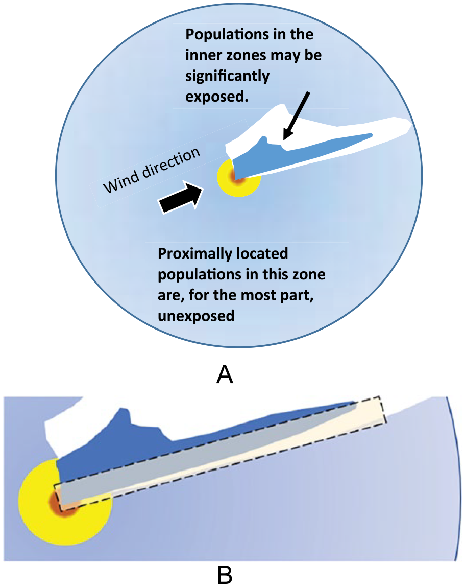
(A) Most proximal locations to radiation dispersal events are relatively unexposed and may be below a threshold requiring triage or medical follow-up. (B) Persons residing in locations near to edges of zones deemed for active triage or medical follow-up have greatest uncertainty and may require additional and more detailed dose analysis (box above).
The value of radiation field maps, developed quickly after an event by aerial radiological monitoring or similar technologies, is of considerable value for assessing group and/or individual exposures. Determinations concerning evacuation levels, triage levels, or any predefined cut-off limit (i.e., what might be called threshold dose assessments) can then be made. In this case, the threshold would be a predetermined value above which a particular action (e.g., evacuation) is justified or required. For this purpose, the depicted map contours can be useful both as a communication device with the public and for public health authorities to determine the geographic area of populations where a response is needed. Clearly there may be zones near to the edge of the threshold areas that will be uncertain, and more careful assessment will be needed (Fig. 7.1B).
7.3 Uses of Radiation Field Maps for Quantitative Dose Estimations
Maps of radiation fields can be obtained by many different measurement devices and technologies not described here. Existing publications (e.g., ICRU, 2002, Report 68; Klemic et al., 2006) discuss radiation field devices and measurements. There are many examples in the literature of radiation field mapping, with the most recent emphasis being on aerial monitoring (e.g., Kim et al., 2008; Sanadaa et al., 2014). Those techniques with the highest precision and spatial resolution will, of course, be of greatest benefit for dose assessments of individuals.
While radiation field maps have the advantages of simplicity and clear visualization, they also have limitations. For example, maps of radiation fields are subject to change with time after the event due to the accumulation of additional data and/or changes in the radiation field itself. Changes could result from (1) change in the radiation field pattern and/or intensity due to continued atmospheric dispersion of a continuing release, or (2) change in the radiation field pattern and/or intensity due to physical decay, weathering, and redistribution of the radioactive materials already released. Examples of radiation field maps were numerous following the Fukushima reactor accident in 2011 and changed with time because additional radioactivity releases changed the radiation field and because additional data were continually being collected. For example, an early map of dose rate following the Fukushima reactor accident is shown in Fig. 7.2A.

(A) Map of 137Cs ground deposition (Bq·m–2), interpreted from aerial survey data on May 26, 2011. (B) Radiological survey map of Fukushima area expressed by areas exceeding recommended relocation guidance levels. (C) Exposure rate (mR·h–1) map near the Fukushima Daiichi reactor complex, April 3, 2011. (D) Dose rate (mSv·h–1) map near the Fukushima Daiichi reactor complex created on April 29, 2011. (E) Integral dose map for 1 year in units of millisievert in the region of the Fukushima reactor accident.
Other maps, produced by Japanese agencies, used data made available from the US National Nuclear Security Administration (NNSA) but supplemented with data collected by other monitoring teams. Two maps from the Japanese Science Ministry follow in Fig. 7.2B and 7.2C, one being in terms of dose rate and another in terms of integral dose.
To use radiation field maps for dose assessment, it is essential that law enforcement and public health authorities understand the units, assumptions, and limitations of the data collected and how they have been interpreted to make the map. Failure to completely understand the physical basis of the data used to make the maps can result in erroneous interpretations. Comprehension of the basis for the maps by the public would also be useful but possibly less important than for authorities who are charged with decision making.
Maps based on a variety of measurement units and assumptions can be found. Some maps, for example, present the spatial pattern of contamination for the activity of a specific radionuclide deposited per unit area on the ground (see, for example, Fig. 7.2A for 137Cs in the environs of the Fukushima accident). Such maps are usually derived from interpretation of aerial gamma-ray spectrometry and have inherent limitations of the spatial resolution of the measurement system and the conditions of its use (e.g., the height above the ground for aerial reconnaissance). An important attribute for contamination maps to understand is that they represent the situation at a specific moment in time. The spatial concentration of the radionuclide on the ground will change with time due to radioactive decay, natural weathering processes, and man-made remediation.
In contrast, some maps present the spatial pattern for areas recommended for relocation (Fig. 7.2B). Other maps present the spatial pattern of air exposure (R) or exposure rate (mR·h–1) (i.e., using conventional radiation measurement unit; see, for example, Fig. 7.2C).
Because there is a considerable lack of understanding among the public about the numerical differences between conventional radiation units and international units, the use of different units at different times or for different audiences could lead to erroneous interpretations. More frequently today, dose maps represent the measurement data in international radiation units, either as air kerma (Gy or Gy·h–1, or Sv or Sv·h–1) or as integral dose to air (Gy or Sv, or Gy·h–1 or Sv·h–1) (see, for example, Fig. 7.2D and 7.2E). Maps showing integral dose to air (e.g., Fig. 7.2E) implicitly integrate the exposure rate over a specific length of time and may be the map type that is most easily subject to misinterpretation if used for dose assessment of individuals or groups.
Regardless of the choice of radiation units, maps are usually derived under the assumptions of an infinite (unobstructed) field. Such assumptions often result from data having been collected at an altitude above buildings and other obstructions. The latter might change the dose rate or integral dose at specific locations on the ground due to partial shielding. Clearly, even moderately realistic estimates of doses to persons would need to consider the location(s) of the person, elapsed time of irradiation, radiation exposure geometry, and degree, type, and shape of shielding (see NCRP, 2009, Report No. 163) between the exposed persons and the source of exposure.
For dose assessments that attempt realism and are based on radiation field maps, the individuals who are the subject of the dose assessment must be determined to have been at a specified location within the mapped radiation field for a specified period. The primary challenge in applying a dose mapping strategy to a dose assessment is to identify the persons exposed within the mapping area, their locations, and the length of their exposure at each location. The simplest strategy for a dose assessment would be for exposed individuals to self-identify as having been in the mapped area at the time of the event and to be able to adequately describe their location(s), including the length of time spent in each location within the radiation environment. In urban environments, physical addresses and/or names and locations of buildings the persons were located when the event occurred would facilitate interpretation of their dose from a dose map.
Dose maps are usually presented as iso-contours implying that there is some range of true dose that individuals might have received depending on how close they were to one contour line or another. However, proximity to one contour line versus another is probably a minor contributor to the overall uncertainty of estimated dose, except in the inner and outer contours.
Generally speaking, for a dose-rate map to be applicable to an individual exposed to radiation from a specific event, the times that the exposure for the person began and ended (relative to the event) must be known, at least approximately. For a member of the public, the beginning of exposure would usually be the time of the incident. The end of their exposure would generally be the time they left the area. Similarly, for a radiation emergency worker who comes into the contaminated area after the event, the beginning of exposure would be their time of entrance in the mapped area and their end of exposure would be the time at which they exited the contaminated area.
Integral dose maps can only be used for dose assessment when persons of interest were within the mapped area for the length of the time integral used to create the map. Included in integral dose maps are the rate(s) of decay of the radiations or radioactivity. To estimate dose using a dose-rate map, the rate of decay of the field must be known so that the integration can properly account for the change in the dose rate.
The uses of dose maps for individual or group dose estimation discussed to this point assume that the exposed person or groups remained at a single location. That is, of course, the easiest scenario to model could possibly represent an upper-bound dose if the location of exposure had the greatest (or near to the greatest) dose or dose rate in the area. In reality, of course, people may move within the radiation field map. Their location during the initial exposure (i.e., at the time of the incident) might be one of higher or lower dose rate than other locations that the person(s) move(s) to. The new locations may have more (or less shielding) or be characterized with higher (or lower) dose rates due to more (or less) contamination. Establishing an upper-bound dose estimate would become most useful when the assessed level of exposure did not require any medical or active intervention, implying that other areas would be lower than the limit requiring intervention.
For more realistic dose assessments using radiation field maps, the locations and lengths of time at each location would be required. This type of data and the associated analysis is usually termed “time-and-motion” dose analysis which was developed in detail for reconstruction of doses to Chernobyl clean-up workers (the “liquidators”; Chumak, 2012; Kryuchkov et al., 2009).
The most basic form of the time-and-motion technique assumes that dose rates stay relatively constant at any single location, at least over periods of time that might characterize the movements of individuals. A relatively simple analytical formulation is used to estimate dose (e.g., air dose or whole-body dose). This is:
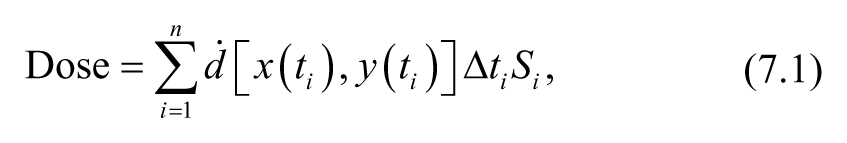
where i is the number of locations at which the dose is summed;
For situations where the dose rate does not stay constant over the integration period due, for example, to radionuclide decay, the functional form of the decay rate must be known or assumed. For example, in the case of a simple exponential decay rate, the dose might be approximated by
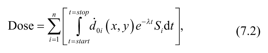
where i is the number of locations at which the dose is integrated;
Dose estimation based on radiation field maps and time-and-motion strategies may need modifying factors to convert measured dose rates in outdoor air to dose for the whole body or to a specific organ. For example, dose conversion coefficients (DCCs) to convert air kerma to body dose or organ dose can be obtained from International Commission on Radiological Protection (ICRP) Publication 116 (2010). Given photon irradiation energies >500 keV, all organs of the body will be irradiated to similar degrees. For low-energy photon radiations, deeper seated organs may receive less exposure than surficial organs. However, differences in true doses received by organs may be less than the overall dose estimation uncertainty. This and related issues are discussed at some length in NCRP (2007; 2009).
In addition to air-kerma-to-organ-dose DCCs, factors may be needed to account for reduction in exposure when indoors or within automobiles [i.e., Si in equations (7.1) and (7.2)]. Dose assessment for those exposed indoors or within automobiles would need to account for shielding by walls of buildings or thickness of the automobile’s metal and/or glass. Shielding factors for buildings of various geometries may be found in Dickson (2013). When the true exposure over the body is inhomogeneous due to diverse shapes and thicknesses of shielding materials between the radiation source and the individual exposed, particularly if the shielding is not well characterized, significantly greater uncertainty in individual dose estimation will occur. Radiation field mapping techniques can, in theory, be supplemented by individual interviews of exposed persons to attempt to elucidate the actual exposure conditions and how they varied from the ideal conditions offered in a radiation field map.
The degree of sophistication of time-and-motion dose assessment strategies can be relatively advanced through the use of supplemental data (e.g., those obtained from interpolation strategies), individual interview data, and the use of numerical techniques to assess dosimetric uncertainty. A well-established method to propagate error on individual doses is to assign probability density functions to each of the model parameters and to propagate the error by Monte Carlo simulation (see NCRP, 2009). Such a strategy is easily manageable with time-and-motion methods since they have few parameters and use a simple, multiplicative analytic form. The studies of Chumak (2012) and Kryuchkov et al. (2009) provide good examples of the use of such strategies to improve dose estimation capabilities over that inherently provided by radiation field maps and time-and-motion techniques.