
Abstract
The study of human activity in space and time is an inherent part of human geography. In order to perform such studies, data on the time use of individuals, in terms of sequence and timing of performed activities, are collected and analysed. A common assumption when analysing individuals’ time use is that groups that exhibit similar background and demographic characteristics also display similarities in how they use their time to structure their daily lives. In this article, we set out to investigate the correctness of such assumptions. We propose a visual analytics process based on sequence similarity measures tailored to event-based data such as performed activity sequences. The process allows an analyst to retrieve similarly behaving records according to user-selected similarity preferences and interactively explore aspects of this similarity in a multiple linked-view environment.
Introduction
The study of human activity in space and time is an inherent part of human geography. A common approach to performing such studies is through the collection and analysis of data on the time use of individuals. Time-use data are collected by statistics companies worldwide through time-use surveys where individuals log their performed activities, in detail, over a period of time. They are, hence, a type of event-based data composed of sequences of time-stamped events (activities). Such surveys aim at mapping the way in which people allocate their time in performing their daily activities and are used in many different areas. Examples of such areas include policy making, where studying the way people structure their daily life can help politicians make more informed decisions, and everyday life research studies, where it can aid in understanding and studying how people live their lives.
Time-use data are usually analysed by computing the proportion of time allocated for performing different activities by different groups of individuals and comparing the time use of the various groups. A common assumption when doing so is that similar people behave in similar ways, which, in practice, means that we consider groups that exhibit similar background, economic and social status, and demographic characteristics to also display similarities in how they use their time to structure their daily activities and thus their lives.
In this work, we set out to investigate the validity of such assumptions by reversing the flow of actions. Instead of extracting groups having similar characteristics (e.g. with respect to sex, age, location, income, and education level), assuming they exhibit similar behaviour and comparing their time use, we let the actual behaviour decide the similarity of individuals. We start from the activities performed and investigate whether people who perform activities in a similar manner in fact display similarities in other characteristics also.
In order for this to be possible, the similarity between individuals’ activity sequences needs to be quantified and measured. Individuals perform a number of activities during the course of each day, and combinations of different activities can, together, define larger activity projects. For example, ‘cooking’→‘eating’→‘doing the dishes’ (where the symbol ‘→’ indicates followed by) can be seen as parts of the project ‘having dinner’. Measuring similarity between individuals in a population includes comparing how they incorporate such projects into their days. When during the day, how many times, for how long, with how many interruptions, and with what kind of interruptions are factors that characterize the way individuals go about their projects and, hence, reflect their daily behaviour. Having this as our starting point, we compare individuals based on how activity projects are distributed in their days and retrieve groups of similar behaviour.
The definition of similarity, however, depends largely on the type of data, the task at hand, and also on the person performing the analysis task. As a result, different attributes of a sequence’s appearance are interesting in the various cases. Furthermore, when dealing with multifaceted event-based data, such as time-use data, there can be many notions of similarity within a single data set. Factors such as event context, meaning what other events are occurring before and/or after an event, duration, and timing in which event-sequences are performed, can be equally as important as the order in which the events are performed. Consequently, the definition of similarity needs to be flexible, so that it can be adjusted to meet the specific purpose of an analysis task, and at the same time, it should be general enough to be applicable to a wide range of areas.
Previous work has primarily addressed methods for the identification and exploration of sequences as patterns in event-based data.1–6 The work presented here focuses instead on the step following the identification of such sequences.
A visual analytics process is proposed for the identification of similarly behaving groups of event-sequences based on how sequential patterns are incorporated within them. A set of similarity measures specially designed for event-based data 7 are used for comparing and clustering event-sequence records. Following this, the resulting clusters and their membership are explored in a set of linked visual representations. These enable the analyst to examine the qualities of the clusters, explore the source of the similarity, and cross-reference the results against any available supporting information, such as meta-information describing additional attributes of the data, in order to further explore aspects of the measured similarity.
The main contributions of this work are as follows:
Definition of a visual analytics process for identifying and exploring groups of similar sequential behaviour based on a user-adjustable similarity definition.
Presentation and use of a set of similarity measures specifically tailored for comparison of event-based data.
Suggested combination of a set of linked displays that allow an analyst to explore different aspects of the identified similarity and cross-reference the correspondence of the clustering results to natural groupings and inherent characteristics of the data.
This work has been centred around the analysis of event-based data in the form of time-use activity diary data; the presented methods, however, are also applicable to other event-based data types. Examples include medical health records, where patient groups with similar conditions may be sought, or process control data, where the objective is to find sequences of events leading to a system failure.
The remainder of this article is structured as follows. Relevant related work is discussed in section ‘Related work‘. In section ‘Data‘, the data used for exemplifying our approach are described. The proposed visual analytics approach is presented in ‘Visual analytics process‘ followed by a discussion of its complexity and a usage example. The generalizability of the method is discussed next and finally conclusions are made.
Related work
This section will review work on the measurement and analysis of similarity in event-based data in the search for similar groups. A widespread approach to measuring similarity in biological sequence data is sequence alignment, 8 which defines the degree of similarity between two sequences by the number of ‘edit operations’ (insertion, deletion or substitution) needed to turn one sequence into the other. The most popular edit distance measures for computing this similarity are the Levenshtein 9 and Hamming 10 distances. Sequence alignment has been introduced to the social sciences 11 to consider several types of event-sequence data such as historical data, careers, travel patterns, and time-use diaries,12–14 and it has even been used for analysing eye-tracking data sequences. 15 Edit distances have also been extended to consider time shifts between compared elements of the sequences and applied to time series. 16 However, edit distances, in general, do not consider fundamental characteristics of event-based data sequences, such as time of occurrence, duration, and context of events, so they may not yield the most useful results. Apart from edit distances, there are a number of alignment-free distance measures for comparing sequences, based on word frequencies and data compression, for example (for a summary, see Mantaci et al. 17 ). Following such similarity measurements, clustering is commonly used to identify groups of similar sequences. There are many examples of tools using clustering and/or visualization and interaction techniques to reveal similarity in biological sequences.18–24 An evaluation of some of the tools most well known to the information visualization community has been presented by Saraiya et al. 25
Similarity in event-based data is often identified using sequence mining 26 and query-matching approaches, and groups are identified visually, often via multiple linked views. Wong et al. 27 identify sequential patterns in documents and explore them in a parallel coordinates like setting. PatternFinder 1 allows the interactive creation of database queries by defining and constraining event-sequences. Similar event-records matching the queries are displayed and visually compared. Lifelines2 makes use of alignment, ranking, and filtering to reveal records showing similar patterns of events with respect to their temporal ordering, 28 and stacked bar charts over a time frame are used to highlight the density of event occurrences. 29 VizPattern 30 is a similar environment for querying and identifying sequential patterns using a comic strip metaphor for the query creation. Session Viewer 31 allows the creation of event-sequences and highlights their matches in order to reveal patterns and similarity within and between web sessions. Recurring patterns of events in the form of hotel visits are identified through an interactive visualization framework by Weaver et al. 32 Zhao et al. 33 make use of three-dimensional (3D) rods over a geographical map and 3D activity ringmaps to display trends of daily activity events. Eye-tracking data sequences are visualized, compared, and explored by Fabrikant et al. 15 and Tsang et al., 34 while personal music histories are considered by Baur et al. 35
Research on similarity metrics specifically for event-based data is not as extensive. A similarity measure for categorical sequence data based on the number of common elements and the order in which these appear is presented by Gomez-Alonso and Valls. 36 In the 2009 article by Wongsuphasawat and Shneiderman, 6 temporal categorical data records are pairwise matched to a chosen or created target record, and a similarity measure is proposed that is based on the time difference (distance) between matched events and the number of missing or extra events compared to the target. This work is comparable to ours in that we too are looking for sequences similar to a ‘target’ subsequence; we, however, also take into account the duration of an event-sequence and its time of occurrence. ARTEMIS 37 is a sequence similarity measure that considers duration of events, which is based on Allen and Ferguson’s 38 model of interval temporal logic. Finally, similarity of event-sequences has been extensively researched by Moen 39 who has proposed an interesting similarity measure for event-sequences based on the context of occurrence of the events making up the sequence.39,40 The context of an event, ei, occurring at time, ti, is defined as the set of all event types that occur within a certain time frame before ti. An event-sequence similarity measure that takes into account the context of events is also presented by Brooks and Memon. 41 We also base some of our computations on this notion of event context. We, however, expand on the factors characterizing an event-sequence and complement the algorithmic approach with an interactive visualization.
In summary, the search for similarity is a common task in event-based data but, while there has been extensive research on identifying groups of similar sequences in biological data, the amount of work on event-based data similarity does not compare. In this work, we measure similarity between event-sequences through a set of measures tailored to event-based data and use clustering to classify a population of records into groups showing similar behaviour.
Data
In order to illustrate the functionality and potential of our methods, we have used an event-based data set consisting of individuals’ activity diaries. However, any data set having a similar structure could have been used instead. The diaries we used were collected in a time-use survey conducted by Statistics Sweden (SCB) during which a representative sample set was invited to participate and asked to fill in time diaries for one weekday and one weekend day. The collected data are composed of 463 individual volunteers aged 10 years or older. The activities in the collected diaries are classified into a hierarchical scheme of about 600 unique numerical codes at 5 distinct levels of detail (LODs) with respect to the description of the activities and grouped into 7 main activity categories: ‘care for self’, ‘care for others’, ‘household care’, ‘reflection/recreation’, ‘transportation’, ‘prepare and procure food’, and ‘gainful employment/education’.
Each event-sequence record in the data is an individual’s activity diary and corresponds to the sequence of activities performed by the individual during the course of a day (what the individuals are doing). The diaries include information about timing and duration of the activities (when and for how long activities occur) as well as the location where each activity was performed (where) and the social context of each (together with whom they are performed). Figure 1 (above) shows a visual representation of a population’s activity diaries. In this representation, each diary is drawn as a stacked bar showing the sequence of activities performed during the 24 h of a day. Time of day is displayed on the y-axis going upward, and the individuals’ diaries are ordered on the x-axis by sex and ascending age from right to left. Colour is used to display the interchange of activities at the most general LOD (seven colours). Sequences of visited locations and changes in social context can also be represented using this representation.
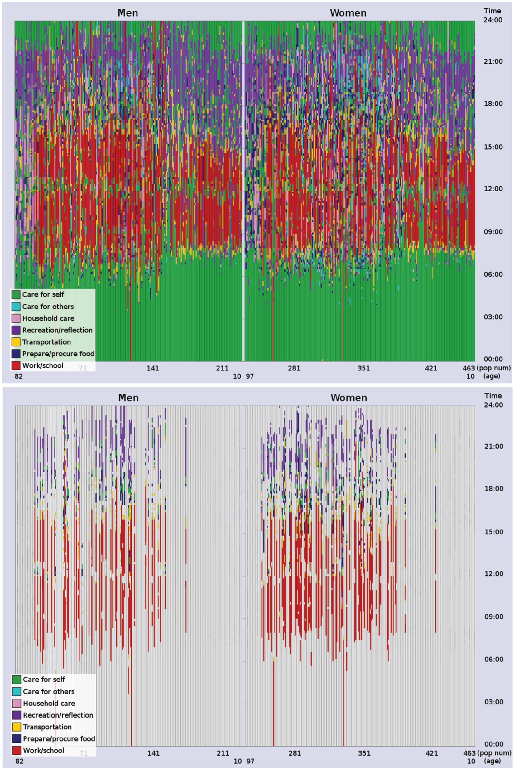
Visual representation of the activity diaries of a population subset. Time of day is displayed on the vertical axis (y-axis), and the individuals’ activity diaries are ordered along the horizontal axis (x-axis) by sex and ascending age from right to left. Colour represents activity category. Top: All activities performed during a day are displayed. Bottom: Activity sequence work→travel→prepare food→eat→private recreation is highlighted.
In addition to the activity diaries themselves, extensive background information about the individuals involved was also collected in the survey. This information includes a list of 36 attributes characterizing each individual. Examples of these are age, sex, region of residence, income, number of adults and children in the household, number of children in daycare, housing situation, employment, education, stress level, perceived health, and also detailed practical information concerning the household such as number of rooms, car ownership, labour-saving devices, and so on. The availability of this extensive metadata is the main reason for choosing this data set for our examples.
Visual analytics process
The visual analytics process we propose for the identification of similarly behaving groups and the interactive exploration of their similarity is implemented as part of a visual analysis tool created for the study of daily life. 42
Interesting sequences of events (activity projects) are used as ‘search-keys’ or query-sequences, and instances of them, query-matches, are located in the data. Similarity between event-sequence records (the individuals) is then computed based on how these query-matches appear in the data and is quantified by means of a set of characteristic sequence attributes (see section ‘Similarity measures for event-sequences’). A user can choose which attributes should be considered in the similarity computation and compose a feature vector of values that describe each record (individual). The individual feature vectors are then clustered, and groups of similar records are retrieved. The cluster membership, clustering quality, similarity measurements, and supplementary information are then explored in a linked-view environment. This whole process is interactively driven by a user/analyst who has influence over the selection of the query-sequence, can define similarity according to the task and preference by selecting which measures to consider, adjusts the settings of the clustering, and interactively explores the resulting groups. So, our proposed visual analytics process includes four main steps that will be described in detail later in this section:
Query-sequence selection.
Similarity measures computation.
Clustering.
Visual exploration.
Visual exploration of the results may give rise to new hypotheses in which case alternative similarity comparisons can be investigated by adjusting the similarity choices and repeating steps 2–4. Before describing the steps of our process, the similarity measures we have used will first be discussed.
Similarity measures for event-sequences
In previous work, we have formulated a set of attributes that describe the way in which a particular sequence of events is expressed in a larger event-sequence record. We have, further, investigated the general applicability of these attributes to various types of event-based data through an interview-based study. 7 These attributes can be quantified and used to assess similarity between records. In this work, we refine and make practical use of these attributes as measures of similarity between individuals’ daily activity sequences.
In our proposed approach, similarity can be measured per record or per query-match. For our activity diary data, per record similarity is chosen when the objective is to compare and group individuals per se, as inseparable entities, while per query-match is chosen when the objective is to study variations of the sequence pattern itself across individuals. When computation of measures per query-match is chosen, a copy of the event-sequence record is created for each of the identified pattern matches.
We have in our previous work 7 described the measures in detail; here we go through them very briefly. We have separated the measures into three classes: (I) ‘record measures’, (II) ‘query-match measures’, and (III) ‘gap measures’, where gap refers to the set of events interrupting a sequence.
Record measures are concerned with the general structure of an event-sequence record and are independent of the query-sequence. 1. Fragmentation refers to the number of events composing an event-sequence; the length of a sequence. 2. Variation refers to the number of unique events composing the event-sequence.
Query-match measures are concerned with attributes of the identified instances of a query-sequence, meaning characteristics of the query-matches. 3. Number of occurrences is the number of identified instances of the query-sequence in a record; the number of query-matches in the event-sequence. 4. Sequence start time refers to the start time of the identified query-match. 5. Event start time refers to the start time of each of the events composing the identified query-match. The measure is defined as a vector of length equal to the query-sequence that stores the start time of each of the matched events. This measure is, at the moment, considered only in the per query-match computation since it focuses on the separate events of a query-sequence. 6. Sequence duration refers to the total duration of an identified query-match, from the start of the first matched event until the end of the last one including any interrupting events. 7. Events duration refers to the sum of the durations of the distinct events composing the identified query-match.
Gap measures deal with the context in which instances of a query-sequence are identified. The context of a sequence is defined as the set of events surrounding or interrupting the sequence. So the gap measures consider characteristics of the events interrupting an identified query-match. 8. Gap size refers to the number of events interrupting an identified query-match; the number of intervening events or gap events. 9. Gap duration refers to the sum of the durations of the events interrupting an identified query-match. 10. Gap type refers to the type of events interrupting an identified query-match. Gap type is saved as a vector of length equal to the number of unique event types (the size of the event-type set) that stores the count of events of each type. In the case of our activity diaries, a vector of length 7 is considered, since there are seven activity categories in which information about the category membership of the gap activities is stored.
Query-sequence selection
The first step of the proposed analysis process is the selection of a query-sequence of interest. If there exist specific habits or sequence patterns that a user wishes to analyse, then the query-sequence can be entered manually. Otherwise, a sequence mining or other sequence identification method could be used for identifying and specifying a query-sequence of interest. The process we propose therefore assumes that interesting sequences of events (activity projects) have been previously identified as patterns using a preferred sequence identification method (numerous examples of such methods exist1,3,4,6). Query-sequences of arbitrary length can be considered in the presented method. In this work, we have used an interactive visual identification tool 4 to identify interesting sequences of activities from our activity diary data.
Once the query-sequence is selected, all instances of it, query-matches, are identified in the data and saved. The records that include this query-sequence create our similarity search space. Figure 1 (bottom) shows an example of how matches to a query-sequence are distributed across a population of activity diary data. In this case, the query-sequence is work→travel→prepare food→eat→private recreation, which was identified as a frequent pattern in our data.
The diary data used in this work have a hierarchical nature that can be considered in the composition of the query-sequences. This implies that these can include activities at different LODs, for example, a query can be composed of the activity ‘wake up’, defined at LOD 2, followed by any ‘care for self’ activity, defined at LOD 5.
Similarity measures computation
Once the query-sequence is selected and located in the data, the analyst can choose which measures to be used and thus define the terms of similarity. Also whether the measures should be computed per record or per query-match is chosen.
The computed similarity measures compose feature vectors and taken together they compile a feature matrix. The similarity measures that are already defined as vectors are concatenated to the feature vector. For measures to be comparable with each other and be combined into a single measure, the values of each measure (each column of the feature matrix) are normalized to be in the range [0, 1]. The matrix is then passed into a clustering algorithm where distances are calculated between the vectors that indicate a measure of similarity between them.
Even though our activity diary data have a hierarchical nature, the resulting feature matrix includes measures at a single hierarchy level. This is because only the activity-type descriptions are aggregated between different levels of detail in the data set we use, not the actual sequence of activities composing the diary. Consider, for example, the following sequence defined at LOD 2: wake up→shower→get dressed→prepare breakfast→eat breakfast. The same sequence is defined at LOD 5 as care for self→care for self→care for self→prepare/procure food→care for self. The start and end times of the activities do not change, only their description detail changes. So a query-sequence defined at LOD 2 as wake up→prepare breakfast is identified once in the sequence, while a query-sequence defined at LODs 2 and 5 as care for self→prepare breakfast has instead three matches. This means that, regardless of hierarchy level at which the matched activities are described, the attributes measured during the similarity computation are at the same hierarchy level.
Clustering
We have chosen to use the K-medoids algorithm for performing our clustering primarily because of its simplicity and its robustness with respect to outliers and noise compared to K-means. 43 Another reason for choosing K-medoids is the fact that it uses the most representative data element as a prototype for each cluster, which is appropriate considering the categorical nature of our activity diary data that consist of indivisible individuals.
Clustering with the K-medoids algorithm involves choosing the number of clusters to be created, k, and assigning initial k medoids. An iterative optimization process then updates the medoids and reassigns the data elements while the clustering quality is improving. 43 A computational disadvantage in this implementation is that the optimization process involves comparing each data element to all others at each iteration. To avoid this, we use a variation of the K-medoids algorithm, presented in Park and Jun, 44 which instead employs an initialization strategy for computing the starting medoids and then uses a local heuristic approach to find which element within each cluster minimizes its clustering cost, and reassign the elements. This method is similar to K-means since the medoid update process operates locally within each cluster giving the approach an advantage in terms of computation time.
The initialization process for selecting the initial k medoids first involves the computation of a distance matrix between all elements in the data, meaning the distances between all feature vectors. We use Euclidean distance, d(i, j), for this. Second, a measure indicating the closeness of each element to all other elements is computed as the sum of the normalized distances
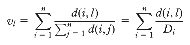
for
We calculate clustering quality, E, in terms of the distance cost of each element, e, to its closest medoid using an absolute error criterion:
An issue to be discussed when using clustering algorithms that require specifying the number of clusters, k, to be created is how k is chosen. In our data, this choice depends on how the selected query-sequence is distributed across the population of diaries, both in terms of frequency of occurrence, which defines the size of the search space, and in terms of the measured similarity between the instances of the query-sequence. Therefore, there cannot be a standard value for k, so in our method, it is chosen through an interactive, iterative testing and adjustment process. This involves the user selecting an initial k, clustering the data, and inspecting the results visually. If these are not satisfactory, with regard to the conciseness of the groups, for example, a new k can be tested instead. This process is possible since the clustering algorithm converges in interactive times.
Weighting factors can be assigned to each of the similarity measures in order to control their influence on the clustering process. These factors are defined by the analyst not as actual values but rather as a relative importance ordering of the individual measures, placing more emphasis on some compared to the others. In practice, this ordering is performed though the interactive adjustment of sliders in the graphical user interface (GUI) of our framework (described in section ‘Visual exploration’). In this way, the analyst can tune the clustering to suit specific search tasks. The weights are normalized such that they sum to one.
Apart from the described K-medoids approach, we have also experimented with other partitioning clustering approaches such as traditional K-medoids with random initialization, bisecting K-medoids, and density-based clustering using OPTICS (Ordering Points To Identify the Clustering Structure).43,45 There are three reasons for our preference for the presented method as opposed to the others tested. First, we prefer to use an initialization strategy in order to have consistent clustering results and avoid the situation where each run of the algorithm results in a different clustering of the data. Second, we prefer to allow the analyst to select the number of clusters to be created and so enable them to adjust the results interactively. This may be considered a drawback under some circumstances, but we have found that the alternative methods tend to identify too many clusters with very slight differences and that, in the case of density-based clustering with OPTICS, too many records end up being considered to be noise. This is also the third reason for preferring the presented clustering approach, namely, that we want all of our records to be clustered even if this results in some clusters being diffuse. This being said, other clustering methods could be used instead within the method we propose.
Visual exploration
We make use of four linked displays (Figure 2) for representing and interacting with the clustering results and a GUI for driving the computations, which includes clustering options and background information selection options.
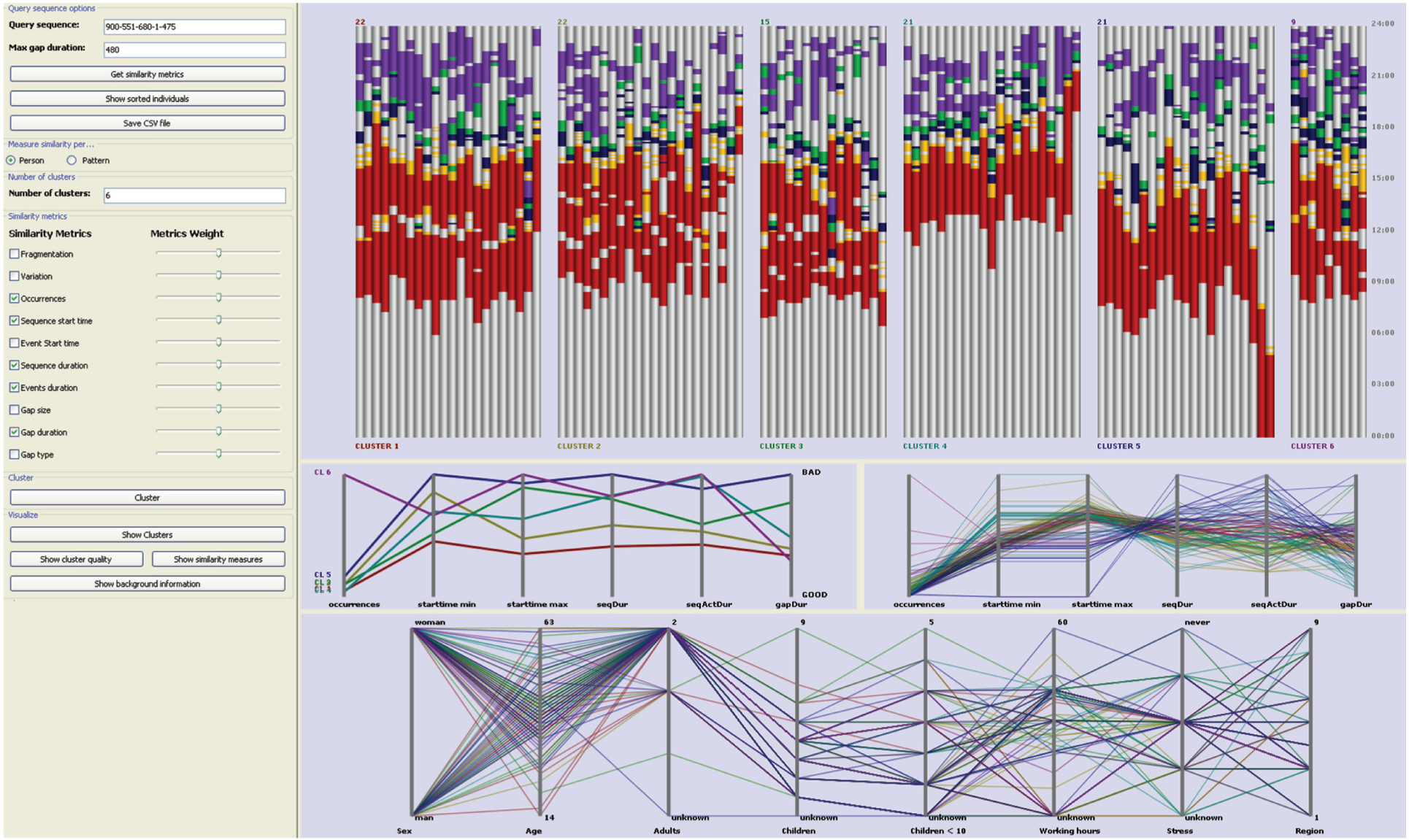
Clustering GUI and clustering results representations. Diaries are clustered per record into six clusters with respect to query-sequence: work→travel→prepare food→eat→private recreation and similarity measures: sequence start time, sequence duration, and events duration. Top: cluster view with highlighted query-sequence. Middle left: cluster quality view showing per measure quality. Middle right: similarity measures view. Bottom: background information window showing additional information about individuals in the clusters.
The clustering options on which the GUI allows decisions are as follows: (1) the maximum allowed temporal gap between adjacent events in the query-matches, (2) the type of similarity to be measured and, hence, the type of clustering (per record or per query-match), (3) the number of clusters, (4) the selection of measures to be used, and (5) the assignment of weighting factors for each. The background information selection options allow the analyst to select which available background attributes to explore. All options in the GUI are implemented using widgets, such as checkboxes, lists, and sliders, in order for them to be simple, easily recognized, and altered even by users of low computer proficiency.
The membership of the clustered event-sequence records can be seen in the cluster view (Figure 2, top) in an in-context visual representation. ‘In-context’, in this case, implies that the results are displayed in the context of the individuals’ diaries in the representation, meaning showing how the query-sequence is incorporated within the event-sequence records. Each bar in the representation corresponds to an individual’s diary, comprising the activities performed during the 24 h of a day. Individuals are displayed on the x-axis, grouped into clusters with spacing to separate them, and time (00:00–24:00) is represented on the y-axis going upward. The same representation could be used for displaying any event-sequence over a certain time interval. The clusters are ordered, from left to right, by their cluster quality, and the individuals within each cluster are ordered, also from left to right, by ascending distance from the cluster’s medoid, which is the first individual from the left in each cluster. The query-sequence matches are highlighted in the context of the individuals’ days allowing the analyst to study their distribution and, hence, understand something of the cluster’s characteristics and coherence. If per query-match clustering is performed, then multiple copies of the same record are shown, one for each identified instance of the query-sequence.
Several parallel coordinate views are used to convey complementary information such as cluster quality (Figure 2, middle left), similarity measure values within each cluster (Figure 2, middle right), and background information corresponding to the individuals in the clusters (Figure 2, bottom). Each cluster is assigned a unique colour that is reflected in all the views: as the colour of the lines in the parallel coordinate displays and as the colour of the clusters’ annotation in the cluster membership display. The cluster quality view shows the per measure quality of each cluster, lines represent clusters, and each coordinate axis corresponds to one similarity measure. The similarity measures view is a parallel coordinates display that shows the actual feature matrix values of each individual in a cluster. The closeness and the range of the values are revealed in this view and hence also the quality of the cluster. The closer the values, the higher the cluster quality. Finally, in the background information window, additional attributes of the data are shown using parallel coordinates. Each line in this representation corresponds to an individual record and each coordinate axis to one of the background attribute values. Which background attributes are to be included in the representation can be selected, altered, and reordered interactively in the GUI.
All views are linked, and selections made in one view are reflected in all others. A cluster can be selected through the cluster view or the cluster quality view, and all members of the cluster in all views will be highlighted. Control-clicking on an individual in the cluster view highlights the individual in the cluster, their feature matrix values, and their corresponding background information, which allows the analyst to access all available information. Ranges of coordinate values can be selected in the background information window by brushing over them to see the individuals’ cluster membership. This allows the analyst to reverse the exploration process by starting from individuals’ personal/background information and the natural groupings they may display and cross-referencing their membership in the clusters while exploring the way in which they perform a certain project.
Finally, information concerning the region of residence of each individual is available in the data making it possible to further analyse the results of our methods in a geographical context. The geographical distribution of the population included in the survey can be displayed across a map, and comparisons between the geographical distributions of individuals in the retrieved clusters can be made. Due to privacy issues, ‘region of residence’ is not collected as exact location but rather individuals have registered whether they live in one of the three largest Swedish cities (Stockholm, Malmö, Gothenburg), in a large city (>90,000 residents), in a medium-sized city (>27,000 residents), in an urbanized rural area (>9000 residents), or in a rural area. Given this information, choropleth maps can be created with information about population count per administrative region of the country. Our framework does not have direct built-in support for geographical visualization, but it is easily adjustable to work in concert with traditional GIS software or sophisticated geovisual analysis frameworks. For this work, we have used the V-Analytics framework. 46
Complexity
The event-sequence similarity–based clustering approach, presented in this article, includes components of varying levels of complexity. The first phase is the location of each instance of the query-sequence in the event data, if this has not already been found during the sequence identification process. This process is approximately linear in the number of individuals, n, represented in the data set, and so the process expands as O(n). The computation of the sequence measures is, similarly, approximately linear in the number of individuals present in the data set since the computation of the measures is carried out within each individual with no inter-individual computation required.
The initialization process for the clustering consists of the creation of the distance matrix and the identification of the initial medoids for the iterative optimization process. The distance matrix is upper-triangular and of size n(n+ 1)/2, where n is either the number of individuals whose diaries include the query-sequence or the total number of instances of the query-sequence in the selected data set, depending on the type of search being made. This part of the procedure expands, therefore, as O(n2). The method used to identify the initial cluster medoids 44 is quite a cheap operation but does expand as O(n3). However, since we are computing the total cost per element variable, Di, during the distance matrix computation, this complexity is reduced to O(n2). The advantage gained from this more complex initialization process is that fewer iterations of the K-medoid optimization procedure (which expands as O(n2)) are required. Overall, therefore, the method expands as O(n2). For the data we have experimented with, which is not very large, the clustering completes in a few seconds. Even with larger data, one has to keep in mind that our proposed method is applied after sequential patterns have been identified in a population and hence acts on a search space that is already initially pruned. Even so, of course, when dealing with very large data sets, the K-medoids approach could become too expensive and an alternative clustering approach with random initialization could be employed instead.
Usage example
In this section, we present a usage scenario in order to demonstrate our method and its functionality. The number of possible searches that can be done within a data set such as the activity diary data considered in this article is, of course, huge, and due to lack of space, we will show only an example of how an exploration can proceed. Considering, furthermore, that these activity diary data aim at describing daily life, the patterns identified and explored may not lead to results that are unexpected. They do, however, provide a proof of concept.
A pattern that was identified as frequent, through the sequence identification functionality of our framework, 4 is the event-sequence: work→travel→prepare food→eat→private recreation. This sequence reflects a typical ‘returning home after work’ pattern comprising travelling home after work, preparing dinner, eating, and then relaxing (commonly through reading or watching TV). The query-sequence, matched in our data without constraints, is performed in total by 124 (of the 463) individuals, 76 women and 48 men. Its distribution across the population can be seen in the ‘in-context’ representation of Figure 1 (bottom) where individuals are ordered by sex and age (women are viewed to the right and men to the left). The increased presence of women becomes directly evident in this representation. Also revealed is the fact that no senior individuals or children are performing the query-sequence, which is due to the inclusion of the activity ‘work’.
We extract the records that include the query-sequence and initiate the clustering process, choosing to compute similarity per record (per individual) using a maximum gap duration of 8 h (480 min) and measures: number of occurrences, sequence start time, sequence duration, events duration, and gap duration. Figure 2 shows the resulting membership, with the query-sequence highlighted, when clustering the data into six clusters. We can directly see some distinct characteristics in the clusters reflecting certain behavioural similarity. For example, the first cluster is composed of individuals having, on average, a single break during their working day (work activity is shown in red), working for equal periods before and after this break, and having long sessions of private recreation (purple) in the evenings. In cluster 2, instead, the individuals have, on average, two breaks during work and short recreation activities in the evenings, while clusters 4 and 5 include mostly individuals working shorter hours without breaks. Browsing through each of the clusters, by clicking on them, allows their coherence, in terms of the measured similarity values, to be inspected through the similarity measures view (Figures 2, middle right, and 3, top right). The values corresponding to single individuals can also be displayed by control-clicking on them. In addition, when selections are made, additional background information corresponding to the individuals are highlighted and can be explored. Figure 3, for example, shows cluster 2 highlighted revealing a quite concise cluster with respect to all measures, consisting of mostly women (only five men) aged 35–45 years (two exceptions) in households consisting of two adults.
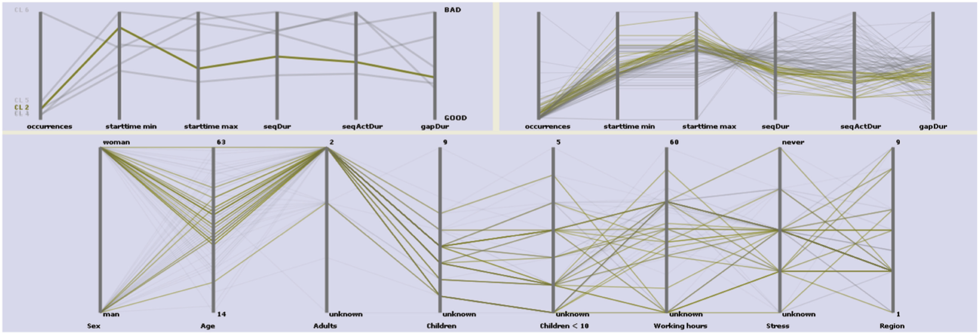
Clustering results representations with a single cluster highlighted.
Including the activity ‘work’ in our search has excluded all individuals older than 63 years and younger than 14 years (as can be seen in the background information window in Figures 2 and 3); we, therefore, remove work from the query-sequence, which becomes now travel→prepare food→eat→private recreation. We cluster again per record into six clusters with respect to measures: sequence start time, sequence duration, and events duration. We use a maximum gap size of 2 h to retrieve more compact patterns, and we assign a weighting order to give most importance to sequence start time followed by events duration and then sequence duration. The results of this clustering can be seen in Figure 4. This query pattern is present more frequently in women than men (55 men, 92 women). Figure 4 (top) shows the clustering results that reveal a distinct grouping of the individuals with respect to start time and duration of events. The average cluster start time is lowest for cluster 6 followed by cluster 2, then 1, 4, 3, and 5. Cluster 3 displays short food preparation (blue) and eating activities (green), and the recreation activities (purple) do not occur continuously during the evenings, they seem interrupted. Cluster 4 is composed of individuals with long-lasting recreation activities, starting on average around 20:00, while cluster 2 includes longer sessions of food preparation and shorter recreation activities starting earlier. Furthermore, cluster 2 is almost entirely composed of women (two exceptions), while in cluster 4, the majority is men, highlighted in the background information and cluster view (Figure 4, middle and bottom). Figure 5 displays the geographical distribution of the individuals belonging to each cluster with respect to their region of residence on choropleth maps. Unclassified colouring has been used on each map (one per cluster) to display the number of individuals per region. Bright colour indicates lower and dark larger number of individuals. Looking at this distribution, we can see that most clusters are composed primarily of individuals living in large cities, apart from cluster 2 in which the majority is from urbanized rural areas followed by rural areas, large cities, and then medium-sized ones. The fact that this is also the cluster composed mostly of women can be seen as indicative of a ‘traditional’ attitude towards division of labour dominating in the more rural areas.
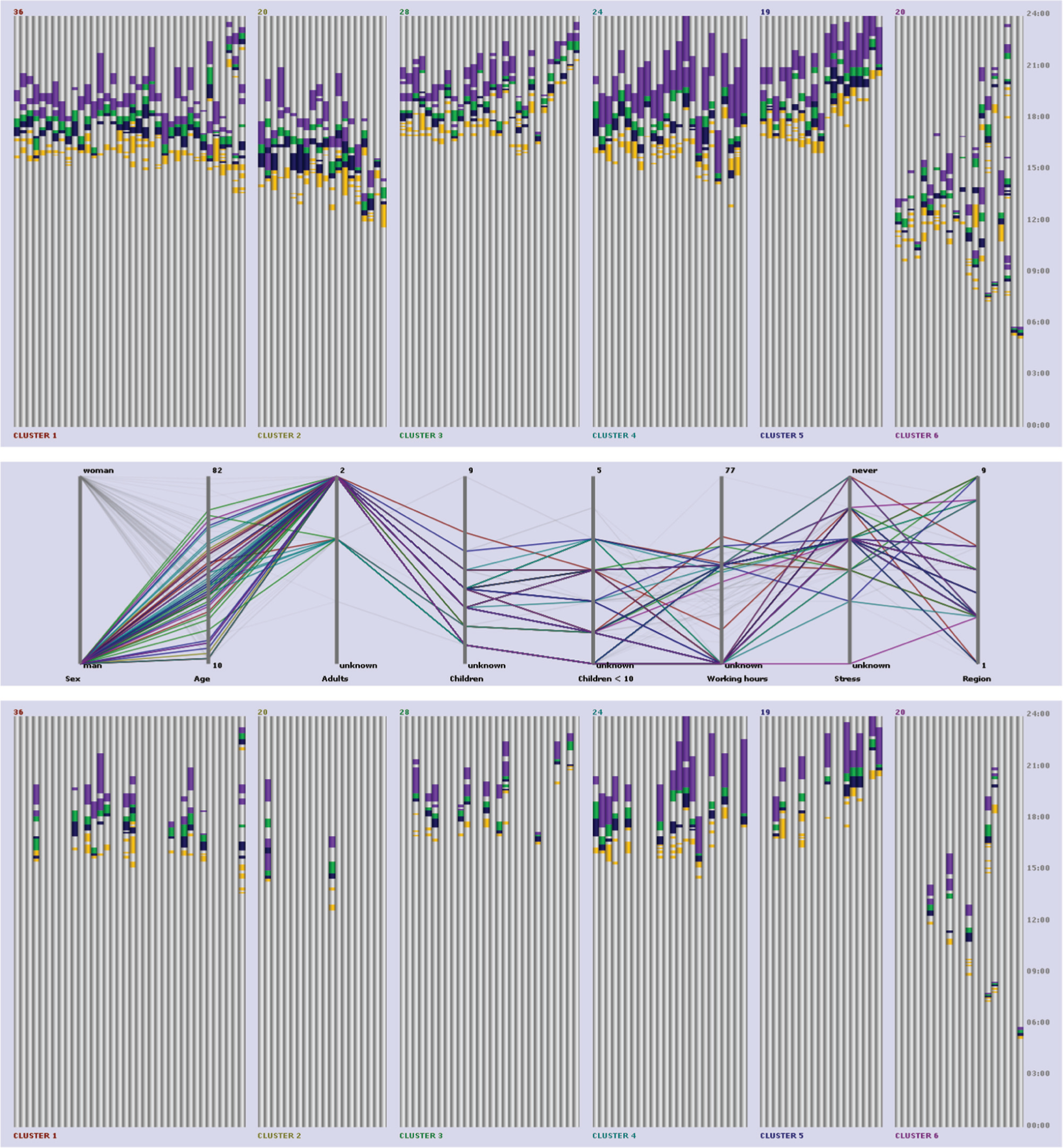
Cluster results of the diaries clustered per record into six clusters with respect to the query-sequence: travel→prepare food→eat→private recreation– and similarity measures: sequence start time, sequence duration, and events duration. Further details can be found in section ‘Usage example’. Top: Cluster view with query-sequence highlighted. Middle: Background information window with male population highlighted. Bottom: Cluster view with male population highlighted.
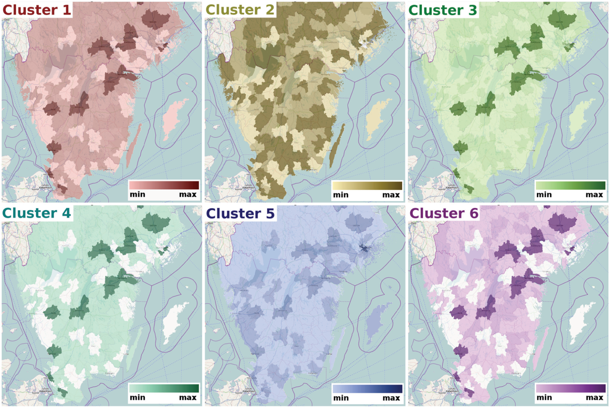
Geographical distribution of the individuals within each cluster with respect to their region of residence is displayed on choropleth maps. Each map corresponds to a cluster, and within it colour signifies the number of individuals per region, bright colour indicates few individuals and dark colour more number of individuals. Only the distribution across the south of Sweden is displayed.
In order to make a final inspection of the unequal distribution of this pattern between men and women, we reduce the query-sequence to include only eat→private recreation and cluster as previously with respect to measures: sequence start time, sequence duration, and events duration but into seven clusters this time (Figure 6, top). As suspected this basic pattern is distributed equally, 215 women and 203 men, and displays more distinct clusters due its simplicity. Clusters 1, 2, 6, and 7 display the pattern on average twice, once earlier during the day and once in the evening but with different starting times and varying duration of the intervening intervals. Clusters 3, 4, and 5 display the pattern on average once, cluster 3 in the morning and the others in the evening with varying total sequence duration. Clustering the data per query-match results in even more concise groupings since single occurrences of each query-match are inspected one at a time. This can be seen in Figure 6 (bottom), which shows the membership results of clustering the data per query-match into 10 clusters with respect to the same query-sequence and measures. Here, distinct pattern variations with respect to duration of activities, duration of entire sequence, and start time become apparent. For example, cluster 1 includes late occurrences of the pattern with very short recreation activities (purple), while in cluster 2, these activities are longer. Cluster 9 instead displays late occurrences of the pattern with long-lasting recreation activities; these activities are also long-lasting in cluster 10, but the pattern in this case has an earlier start time.
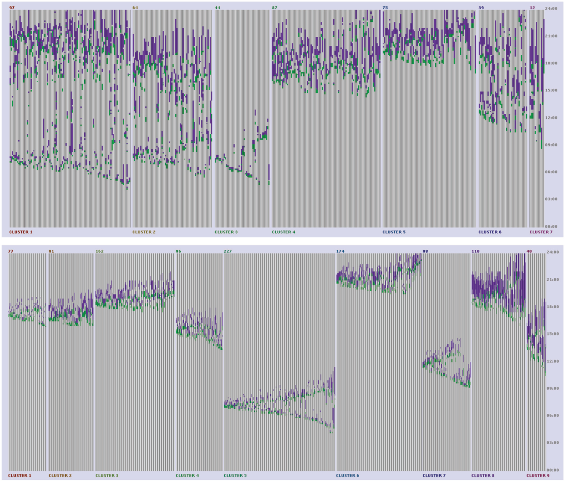
Cluster view of the diaries clustered with respect to the query-sequence: eat→private recreation and similarity measures: sequence start time, sequence duration, and events duration. Further details can be found in section ‘Usage example’. Top: Clustered per record into seven clusters. Bottom: Clustered per query-match into nine clusters.
These very brief descriptions cover just part of what was a much longer exploration process. Weights can be varied to prioritize the effect of the measures. The specific number of clusters to use and the choice of measures to employ are also factors which the analyst can tune during this process. Furthermore, measures can be explored one at a time to reveal more distinct similarities with respect to each of the attributes. Each run of the clustering algorithm takes seconds, so the exploration can continue freely and give rise to new hypotheses to be investigated, enabling the analyst to continue along new exploration paths.
Generalizability
The visual analytics process presented in this work is exemplified using activity diary data. Activity diaries, however, are merely one type of event-based data that are encountered daily in a wide variety of diverse fields. Such data sets consist of sequences of ordered events where each event has a type, a time-stamp, and often a duration associated with it. Examples of event-based data, apart from time-use diary data where the events are activities performed by individuals, also include medical health records where events are medical observations or treatments, internet surfing records where the events are website visits, and administrative and industrial process data where each step of a process is considered an event. In general, any data set that is described by sequences of discrete events occurring in time can be considered event-based data. Having this in mind, the methodology we present is applicable to a wider range of fields where patterns are sought as subsequence of events, and groups of similar records need to be explored.
An issue that needs to be addressed in generalizing our approach is the fact that in activity diary data, all records are of equal length. This can be overcome by considering relative instead of exact time and aligning all records by their first occurring event as suggested, for example, by Wang et al. 28 Furthermore, by not including measures that consider duration, the method becomes applicable to data sets of instantaneous events; alternatively, if the duration is not explicitly specified, it could be derived as the time span before the start of the next event.
Conclusion
We have introduced the use of a set of event-sequence similarity measures that enable the computation of contextual similarity in event-based data and shown their use within individuals’ activity diaries. These measures combined with user-controlled clustering and interactive exploration techniques allow the extraction and explorative analysis of groups exhibiting similar behaviour with respect to a query-sequence.
The methodology we have presented adopts a simplified approach aiming at taking into account the entire set of attributes identified as characteristic of an event-sequence. 7 Further experimentation with the measures themselves and the way they are combined into a single measure is needed to refine our approach. Furthermore, experimentation with additional clustering approaches needs to be investigated in order to deal with the scalability issues of K-medoids.
The two major advantages of this approach are as follows: First, the fact that the analyst can interactively adjust all clustering settings by trying out combinations of measures and their accompanying weights in order to interactively define similarity and explore different aspects of this similarity within the data depending on purpose and interest. Second, it allows for a bidirectional exploration, the analyst can either start from the identified similarly behaving groups and explore their members’ characteristics or start from the individuals in the data and explore how different natural groupings, such as groups of same age, sex, and income level, are distributed in the clusters, meaning how they behave with respect to their performed activities. The combination of these two approaches offers a more exhaustive analysis as well as even more informative results.
Footnotes
Funding
This research has been funded by the Swedish Research Council Formas.