Untangling origin-destination flows in geographic information systems

Abstract

Origin–destination flow maps are a popular option to visualize connections between different spatial locations, where specific routes between the origin and destination are unknown or irrelevant. Visualizing origin–destination flows is challenging mainly due to visual clutter which appears quickly as data sets grow. Clutter reduction techniques are intensively explored in the information visualization and cartography domains. However, current automatic techniques for origin–destination flow visualization, such as edge bundling, are not available in geographic information systems which are widely used to visualize spatial data, such as origin–destination flows. In this article, we explore the applicability of edge bundling to spatial data sets and necessary adaptations under the constraints inherent to platform-independent geographic information system scripting environments. We propose (1) a new clustering technique for origin–destination flows that provides within-cluster consistency to speed up computations, (2) an edge bundling approach based on force-directed edge bundling employing matrix computations, (3) a new technique to determine the local strength of a bundle leveraging spatial indexes, and (4) a geographic information system–based technique to spatially offset bundles describing different flow directions. Finally, we evaluate our method by applying it to origin–destination flow data sets with a wide variety of different data characteristics.

Keywords

Edge bundling geospatial visualization geographic information systems flow mapping edge clustering

Introduction

Origin–destination (OD) flows reflect relationships (flows) between locations in space and are typically created by monitoring movement activities or more abstract relationships, such as trade and information flows. Movement OD flows describe the dynamics between different spatial locations and are therefore widely used in city planning and cartography. We can distinguish between two types of OD flow data: point-based flow data, such as GPS trajectories from mobile devices,¹ with an unlimited number of potential OD locations, and area-based flow data, such as migration between districts, where OD locations are limited to pre-defined areas (often represented by their area centroid). On a more abstract level, OD flows can be regarded as a special case of directed graphs, where vertices (nodes) represent spatial locations and weighted directed edges represent the flows. What makes this type of graph a special case is that the nodes reflect locations in space; thus, their relative positions are of importance to realistically represent geographic patterns.

Visualization has become an important factor in understanding and analyzing OD flows, since a visual representation of these flows is an intuitive way to communicate and study both geographic and directional patterns. The visualization of OD flows is, however, notoriously difficult. When depicting flows as lines, even data sets with a low number of connections soon appear like a cluttered “ball of yarn” and are hard to interpret² as illustrated in Figure 1. To address this issue, the data visualization and cartography communities have been working on methods to reduce visual clutter, for example, by employing vertex clustering,³ matrix,⁴ and grid-based⁵ approaches, showing only partial information,⁶ or glyph-based visualizations.¹ Another prominent method for clutter reduction in graph visualizations is edge bundling. Edges that traverse similar paths can be bundled to reduce the number of lines that have to be drawn and consequently reduce the visual clutter.

Figure 1.

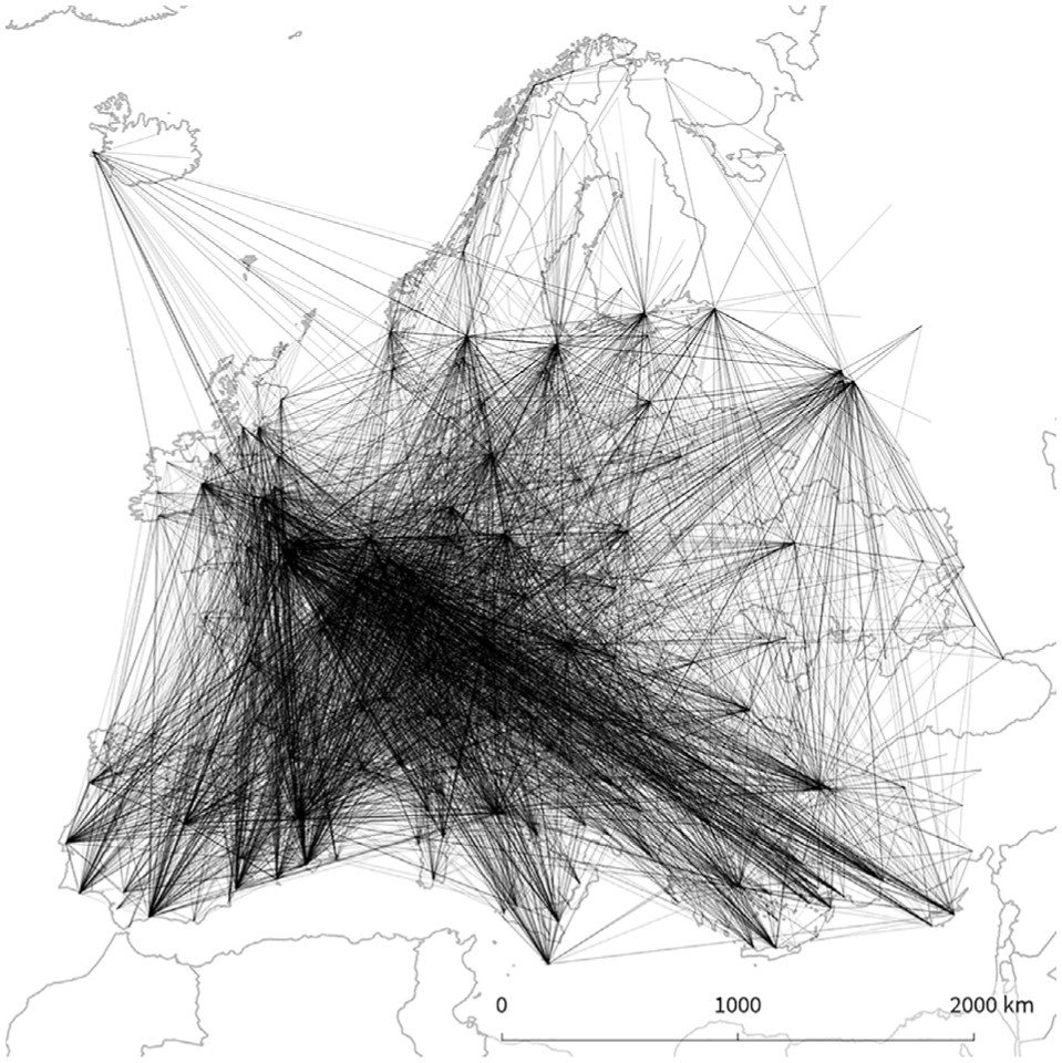
Flights Europe. This point-based OD data set consists of 15,812 edges representing flight connections between European airports.

Researchers have implemented a variety of edge bundling methods which are, for example, based on geometry,⁷ hierarchically organized,⁸ or based on a physical simulation model.⁹ Many of the approaches proposed earlier ignore the flow direction, an issue that was addressed by Selassie et al.¹⁰ by employing edge bundling for directional networks. Since performance is an important factor, especially when analyzing large graphs, Zielasko et al.¹¹ proposed clustering and parallelization to be able to integrate edge bundling in an interactive visual analysis framework.

The goal of this article is to describe the application scenario of applying edge bundling to OD flows using common geographic information systems (GIS) technology—particularly the open-source application QGIS—and a platform-independent implementation. Although already well-studied in the area of visualization, edge bundling is a relatively new concept in GIS. This is on one hand due to the lack of open-source implementations of edge bundling techniques for common GIS applications, but also due to the fact that the findings from the visualization community are not directly transferable to existing GIS applications. Most notably, the use of algorithms running on the graphics card (e.g. in physics engines) is not applicable due to the scripting language nature and platform-independency of GIS scripting environments. Furthermore, the current implementation of the QGIS 2.18 geoprocessing framework does not provide support for parallelization.¹²

Our approach is based on the real-time implementation of force-directed edge bundling (FDEB) proposed by Zielasko et al.¹¹ In general, the FDEB algorithm computes forces along and between edges to bundle compatible edges closer together. Zielasko et al.¹¹ propose an initial clustering step using DBSCAN to reduce the computational effort for calculating edge compatibility. We build on this approach and adapt it to a GIS framework. Our contributions are as follows: (1) We propose a new edge clustering technique based on k-means that automatically determines the optimal number of clusters 2. We use analogies from matrix computations to speed up FDEB calculations by limiting the number of necessary loops and copy operations. This makes our approach very well suited for scripting language environments. (3) In order to enable rendering of resulting bundles using their local strength, we extend the approaches of Selassie et al.¹⁰ and Zielasko et al.¹¹ to add the local bundle strength to the individual segment attributes. We demonstrate how applying a line offset in the GIS visualization resolves the issue that FDEB cannot be applied to convey the direction of edges.¹² This is necessary since pairs of bundles between similar locations but with different directions are placed at the same spatial positions and therefore occlude each other if no suitable countermeasures are implemented.

According to Schumann and Tominski,¹³ visual analytics frameworks for geo-visual analytics should provide (1) an analytic component, (2) a visual component, and (3) an interactive component. By this definition, GIS qualifies as a type of geo-visual analytics system with spatial analysis, map rendering, and map interaction. But stemming from an age of small and usually static data, GIS stands to gain from new visualization approaches in order to avoid clutter when dealing with movement data. Our edge bundling approach addresses the first two geo-visual analytics framework components of analyzing the data and computing visual aggregation. The third component, interactivity, is provided directly by the geographic information system and covers functions including but not limited to filtering flows by attributes, location, or time. By implementing our proposed edge bundling approach as a GIS-based tool, we can leverage existing data reading and writing, spatial indexing, and rendering functionality. Furthermore, our tool is directly applicable to a wide range of GIS data and can be incorporated seamlessly into existing GIS workflows. This broadens the range of influence of our tool beyond the core visual analytics community and closer to the end users of the visualizations.

The remainder of this article is structured as follows: Section “Related work” provides an overview of related work focusing on edge bundling for OD flows. Our enhanced edge bundling method for OD flows is introduced in section “Methodology.” The implementation is described in section “Implementation.” We then present the results from applying our method to multiple data sets in section “Results,” before we discuss the findings in section “Conclusion and future work” together with possible directions for future work.

Related work

Reducing visual clutter is one of the main challenges we encounter when drawing OD flows. Several techniques have been developed to visually aggregate large data sets.¹⁴ For OD flows, the most important flow patterns¹⁵ can be extracted and filters¹⁶ or aggregations⁵ can be applied to generate visually legible OD flow maps. Since the main focus of this article is on edge bundling, we provide a review of relevant existing techniques in the first part. We also make use of clustering to reduce the computational effort of the bundling process. Therefore, clustering techniques are discussed in the second part.

Edge bundling is a well-known approach to reduce visual clutter in line-based visualizations. For a general overview concerning edge bundling in graphs, parallel coordinate plots, and flow maps, we refer the reader to the survey by Zhou et al.¹⁷ and to the detailed report by Lhuillier et al.¹⁸ With respect to OD flows, different approaches can be found in the literature for reducing visual clutter by bundling edges. Edges can be bundled based on geometry, such as routing them through a regular grid,¹⁹ or a mesh generated from the input graph structure.⁷ Others employ hierarchical approaches^8,20,21 to bundle edges on multiple layers. Edge bundling methods alone do not account for bundled properties of the edges (such as quantities).²² Researchers therefore found new ways to communicate additional information of the bundles. For example, Pupyrev et al.²³ draw edges in a bundle in a metro map style to visually convey the number of edges that were combined into one bundle. A comprehensive study by Holten et al.²⁴ shows the effectiveness of different edge representations to convey directions in a graph but not all approaches are applicable to edge bundles. Therefore, Selassie et al.¹⁰ employ color gradients (also known as intensity-based representations²⁴) to encode direction. Other approaches ensure that bundled edges reveal a clearer, and more correct impression of the graph. Ersoy et al.²⁵ used techniques from medical visualization to draw a skeleton of the bundles, which results in a smoother representation of the bundles. Luo et al.²⁶ and Bach et al.²⁷ introduced new drawing styles for bundles to remove ambiguities in the visualization. An edge bundling approach focusing on crossing-free flow maps is so-called spiral trees as described by Buchin et al.,²⁸ but the integrated creation of several flow trees while minimizing crossings between branches of different trees is an ongoing research topic.^29,30 Hurter et al.³¹ present an interactive tool that locally deforms a bundled layout into an unbundled one or conversely, thus helping users to explore the data in more detail. The performance of edge bundling algorithms can be greatly improved by parallelization, typically implemented on the graphics card.³² For example, Wu et al.³³ and Telea and Ersoy³⁴ used image- and texture-based techniques, implemented on the graphics card, to bundle edges. We also employ a matrix-based implementation, similar to the technique proposed by Wu et al.,³³ to avoid loops in the implementation and consequently improve the performance. In the platform-independent scripting language environment of GIS applications, we are, however, not able to make use of parallelization on the graphics card.

Holten and Van Wijk⁹ employed a model based on a physical simulation where forces between the edges are computed. Their FDEB algorithm attaches spring forces (along the edge) and electrostatic forces (between edges) that attract edge points and move them closer together. Forces are only computed (and consequently bundles are only created) between edges that are compatible. The authors introduced several measurements (e.g. based on edge direction and edge length) to calculate the compatibility factors between edges. Selassie et al.¹⁰ later addressed the issue that FDEB does distinguish between edges with opposing directions. With their divided edge bundling technique, only edges with the same direction are bundled. The authors also proposed a method for slightly bending bundles between similar locations, but with different directions, so that bundles are not occluding each other. Peysakhovich et al.³⁵ extended this idea so that edges can be bundled based on direction, or also other attributes. FDEB has a quadratic runtime depending on the number of edges, and therefore does not scale to large data sets. To be able to integrate the algorithm into real-time applications, Zielasko et al.¹¹ avoid using a full pairwise comparison by splitting the set of input edges into separate clusters and calculating FDEB separately for these clusters. Similar to this approach, we also employ clustering to reduce the computational complexity of the edge bundling process.

Clustering of spatial data is a well-researched field in visualization and geographic science.³⁶ Clustering seeks to identify homogeneous groups of objects in a data set. For spatial data, the location and extent of the objects need to be taken into account.³⁷ Spatial data sets can quickly become very large, and spatial clustering is a popular technique for dimensionality reduction. Trajectories, that is, paths that usually reflect movement data, can be grouped by clustering^38,39 to better depict patterns in the data. Ferreira et al.⁴⁰ used analogies from vector-fields to cluster trajectories based on their directions. For OD data, Bouts and Speckmann⁴¹ proposed an edge clustering algorithm based on the compatibility measurements by Holten and Van Wijk,⁹ where users can vary a parameter to define how likely edges are clustered together. We propose a new clustering technique based on KMeans⁴² to cluster the OD flows, which we combine with a measure for cluster variability, so that we can automatically identify the optimal number of clusters.

Methodology

Our edge bundling methodology has three modular steps. The first step is to cluster input edges. While optional, clustering makes it feasible to deal with larger numbers of input edges since subsequent edge bundling is considerably faster: it avoids computation of compatibility between large numbers of heterogeneous edges. The second step is actual edge bundling and comprises determining edge compatibility and modifying edge geometries. The final third summarization step determines the local strength of a bundle which can be used for analysis and visualization purposes. Figure 2 illustrates the three steps for a simple example with only one cluster comprising three edges. We use two visual cues to encode the direction of bundles: First, a color gradient from dark to light encodes the direction of the flow. Second, flows with different direction are offset in the visualization to avoid occlusion and stronger bundles are drawn above weaker ones to further reduce visual clutter and emphasize strong connections.

Figure 2.

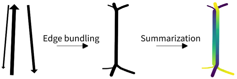
Workflow steps for an example with one cluster with three edges. Line width is scaled by flow strength. Direction in the final result is encoded using a gradient from dark to light.

We implement these clustering, edge bundling, and summarization algorithms as modular tools within the open-source GIS geoprocessing framework QGIS Processing.¹² This framework supports custom scripts written in Python, which can be combined with existing algorithms and used in automated geoprocessing workflows.

Clustering

Good clustering significantly reduces the computation time of later edge bundling steps, because each cluster is evaluated separately, thus making the individual bundling problems smaller.¹¹ This helps with the quadratic computation time. Ideally, clusters should partition the input edges into groups of edges that will be compatible during edge bundling.

In our experience, density-based algorithms, such as DBSCAN⁴³ (used by Zielasko et al.¹¹) and OPTICS, are not suitable because they do not provide within-cluster consistency¹ and—particularly for flow maps—few clusters tend to contain the majority of edges. Table 1 illustrates this issue using Euclidean distance clustering results for a matrix of origin and destination x and y coordinates ( $x_{o}$ , $y_{o}$ , $x_{d}$ , $y_{d}$ ): DBSCAN tends to assign the vast majority of edges to the biggest cluster. This defeats the purpose of edge clustering since compatibility has to be computed for a giant cluster of heterogeneous edges again. DBSCAN’s tendency toward one giant cluster can be reduced by decreasing the allowed distance. However, reducing the distance results in a strong increase in the number of clusters and can thus negatively impact the usefulness of the edge bundling process as discussed in section “Results.” In contrast, k-means distributes the edges much more evenly.

Table 1.

Comparison of DBSCAN and k-means clustering for sample data set of OD in Vienna (n = 1602).

DBSCAN eps/k-meanstarget size	DBSCAN		k-means
DBSCAN eps/k-meanstarget size	# Clusters	# edges in top 3 clusters	# Clusters	# edges in top 3 clusters
1000 m	913	58, 37, 36	266	17, 15, 14
2000 m	77	1307, 40, 29	118	31, 26, 26
3000 m	11	1537, 25, 23	65	55, 53, 47
4000 m	4	1589, 7, 5	39	69, 67, 66

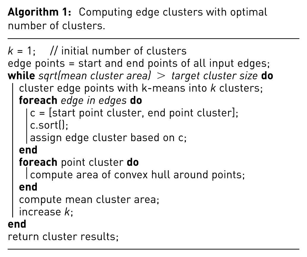
We therefore use k-means to cluster the input edges. We first cluster the merged set of edge start and end points. Then, each unique combination of point clusters—irrespective of the order—represents an edge cluster. The downside of k-means is that it requires a target number of clusters. Instead of having the user decide on the number of clusters, we propose the heuristic approach outlined in Algorithm 1 to determine an optimal number of point clusters. The optimal point cluster number (for our purposes, not strictly mathematically) is the lowest number of point clusters where the start and end points are sufficiently close to each other. More specifically, we determine the square root of the mean area of the convex hulls around the edge points in each point cluster. The number of point clusters is increased until the mean area value drops below the target cluster size, and at this point, the cluster results are considered to be optimal. Figure 3 illustrates this approach for a simple example where the mean area of the two-point cluster solution ( $k = 2$ ) is above the target cluster size. Increasing the number of point clusters to $k = 3$ results in an increase of corresponding edge clusters from 2 to 4.

Algorithm 1: Computing edge clusters with optimal number of clusters.
k = 1; // initial number of clusters edge points = start and end points of all input edges; while sqrt(mean cluster area) > target cluster size do cluster edge points with k-means into k clusters; foreach edge in edgesdo c = [start point cluster, end point cluster]; c.sort(); assign edge cluster based on c; end foreach point cluster do compute area of convex hull around points; end compute mean cluster area; increase k; end return cluster results;

Algorithm 1: Computing edge clusters with optimal number of clusters.

k = 1; // initial number of clusters
edge points = start and end points of all input edges;
while sqrt(mean cluster area) > target cluster size do
cluster edge points with k-means into k clusters;
foreach edge in edgesdo
c = [start point cluster, end point cluster];
c.sort();
assign edge cluster based on c;
end
foreach point cluster do
compute area of convex hull around points;
end
compute mean cluster area;
increase k;
end
return cluster results;

Figure 3.

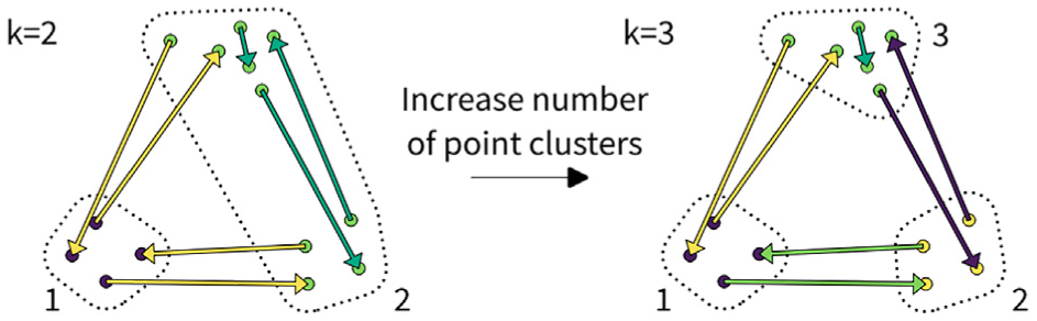
Edge clustering example. Clusters are color-coded. By increasing the number of point clusters k from 2 to 3, the number of corresponding edge clusters is increased from 2 to 4.

Edge bundling

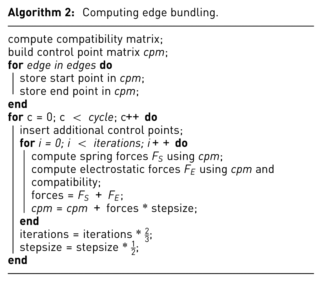
To bundle the edges, we employ FDEB as described by Holten and Van Wijk.⁹ FDEB operates on so-called control points of an edge and applies spring and electrostatic forces to move the control points closer together. The control points of an edge are initialized with the start and end point given by the OD flow. The forces are computed in several cycles, and in each cycle, additional control points are added to the edges. Spring forces are computed between control points of the same edge, and electrostatic forces are computed between control points of different edges.

FDEB only affects edges that are compatible. Holten and Van Wijk⁹ therefore introduced a pairwise edge compatibility measure consisting of four elements: angle compatibility CA, scale compatibility CS, position compatibility CP, and visibility compatibility CV. To compute the compatibility, edges are interpreted as vectors, pointing from their start to their end point.

The angle compatibility CA of two edges ${\vec{e}}_{i}$ and ${\vec{e}}_{j}$ is computed as the absolute dot product of the edges

CA = | ({\vec{e}}_{i} * {\vec{e}}_{j}) | = | \cos (α) | \in [0, 1]

(1)

The scale compatibility CS compares the length of the two edges and is computed as

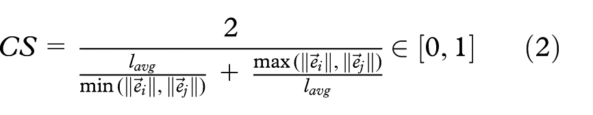
CS = \frac{2}{\frac{l_{avg}}{min (∥ {\vec{e}}_{i} ∥, ∥ {\vec{e}}_{j} ∥)} + \frac{max (∥ {\vec{e}}_{i} ∥, ∥ {\vec{e}}_{j} ∥)}{l_{avg}}} \in [0, 1]

(2)

with $l_{avg}$ being defined as $l_{avg} = (∥ {\vec{e}}_{i} ∥ + ∥ {\vec{e}}_{j} ∥) / 2$ .

The position compatibility CP ensures that edges which are far away from each other are not bundled and is computed as

CP = \frac{l_{avg}}{l_{avg} + ∥ E_{i} - E_{j} ∥} \in [0, 1]

(3)

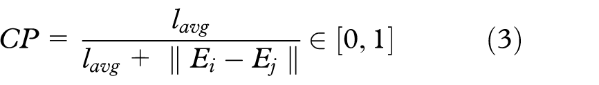
with $E_{i}$ and $E_{j}$ being the midpoints of the edges ${\vec{e}}_{i}$ and ${\vec{e}}_{j}$ .

The visibility compatibility criterion CV ensures that parallel edges with similar length and position are not bundled if they are offset (e.g. like on a parallelogram). It is computed as

CV = \min (V ({\vec{e}}_{i}, {\vec{e}}_{j}), V ({\vec{e}}_{j}, {\vec{e}}_{i}))

(4)

with $V ({\vec{e}}_{i}, {\vec{e}}_{j})$ defining the visibility of an edge ${\vec{e}}_{i}$ to an edge ${\vec{e}}_{j}$ according to the formula given in the work by Holten and Van Wijk.⁹

The compatibility $C ({\vec{e}}_{i}, {\vec{e}}_{j})$ of two edges ${\vec{e}}_{i}$ and ${\vec{e}}_{j}$ is computed as the product of all compatibility measures

C ({\vec{e}}_{i}, {\vec{e}}_{j}) = CA \cdot CS \cdot CP \cdot CV \in [0, 1]

(5)

The compatibility of two edges is symmetric with $C ({\vec{e}}_{i}, {\vec{e}}_{j}) = C ({\vec{e}}_{j}, {\vec{e}}_{i})$ . We use this symmetry to reduce the computational effort by only checking edge pairs once and to store the compatibility values in a two-dimensional (2D) matrix.

In the FDEB algorithm by Holten and Van Wijk,⁹ the number of control points between the start and the end point of every edge is doubled with every new cycle. The new control points are distributed equidistantly along the edge and the old set of control points from the previous cycle is dismissed. This results in an evenly spaced set of control points for every edge (Figure 4(b)). We propose an incremental control point sampling approach where new control points are added in the middle of two existing control points, and control points from the previous cycle are retained. Since in every iteration points of different edges are moved closer together, the control points are pushed toward the centroid of the bundle. The control points are therefore not evenly spread across the edges (Figure 4(c)). This leads to a stronger bundling effect, with edges of one bundle being placed on top of each other. This is desired in our case, since this behavior supports the calculation of the bundle strength in the following summarization step.

Figure 4.

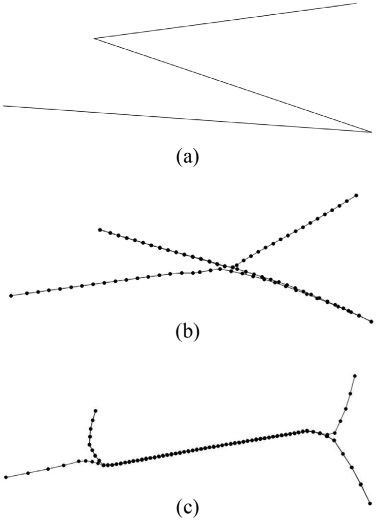
Control point placement. Incremental point sampling retails control points from the previous cycle and adds new points. In every iteration, edges are moved closer together, which, in comparison to equidistant point sampling (b), results in a stronger bundling effect (c), and larger gaps between the control points near the edge ends: (a) input edges, (b) equidistant control point sampling, and (c) incremental point sampling retaining previous control points.

As explored by Holten and Van Wijk⁹ and confirmed by Selassie et al.,¹⁰ it is only necessary to consider forces across edges between control points with the same index. These point-wise relationships of the FDEB algorithm provide several possibilities for improving the performance of the algorithm. Wu et al.³³ suggested to arrange edge control points in a 2D matrix, since all edges in a cycle consist of the same number of control points. The total number of cycles is known beforehand, so the total amount of memory necessary to store the matrix can be pre-allocated. We also employ this approach of arranging the edges in a 2D matrix, referred to as control point matrix $CP M_{m, n}$ in the following. CPM rows represent edges and columns represent control points along the edges.

With the CPM in place, spring forces $F_{S}$ are computed along rows and electrostatic forces $F_{E}$ are computed along columns. Wu et al.³³ shift the last points of the edges in every cycle, whenever new control points are entered into the matrix, until the matrix is eventually filled up. We propose a different approach, where control points always have a fixed position inside the edge-point matrix. This way, we can avoid copy operations in every cycle and only perform value updates instead.

The number of rows m of the CPM is equal to the number of edges $e_{c}$ in a cluster c, resulting in $m = e_{c}$ . The number of columns n can be initialized according to $n = 2^{γ} + 1$ , with $γ$ being the maximum number of cycles. n includes the start and end points. The maximum number of control points differs from the numbers given by Holten and Van Wijk⁹ due to the different approaches we employ for adding new control points, as discussed previously.

During computation, the index p of a control point has to be mapped to a position inside the CPM, defined by the row and column indexes k and l. The indexes can be computed according to the maximum number of cycles. The row index k of a control point is defined by the index of the edge $id x_{e}$ , resulting in $k = id x_{e}$ . The column index l of a control point can be computed as

l = \frac{p}{n_{p} - 1} \cdot (n - 1) = \frac{p}{n_{p} - 1} \cdot 2^{γ}

(6)

with $n_{p}$ being the number of current control points. The structure of the CPM and the computation of the forces is illustrated in Figure 5. The edge bundling algorithm is summarized in Algorithm 2.

Figure 5.

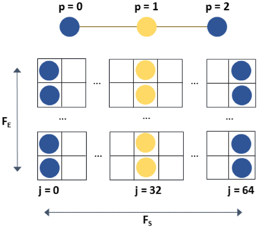
Control point matrix (CPM). An intermediate configuration of the matrix with three control points for every edge is shown. The rows of the matrix represent the edges, and the columns represent corresponding control points positions (start and end points in blue, newly created control point in yellow). The maximum number of cycles $γ = 6$ results in a maximum number of columns of $n = 64$ . Spring forces $F_{S}$ are computed for every row, and electrostatic forces $F_{E}$ are computed for every column.

Algorithm 2: Computing edge bundling.
compute compatibility matrix; build control point matrix cpm; for edge in edgesdo store start point in cpm; store end point in cpm; end for c = 0; c < cycle; c++ do insert additional control points; for i = 0; i < iterations; i++ do compute spring forces $F_{S}$ using cpm; compute electrostatic forces $F_{E}$ using cpm and compatibility; forces = $F_{S}$ + $F_{E}$ ; cpm = cpm + forces * stepsize; end iterations = iterations * $\frac{2}{3}$ ; stepsize = stepsize * $\frac{1}{2}$ ; end

Algorithm 2: Computing edge bundling.

compute compatibility matrix;
build control point matrix cpm;
for edge in edgesdo
store start point in cpm;
store end point in cpm;
end
for c = 0; c < cycle; c++ do
insert additional control points;
for i = 0; i < iterations; i++ do
compute spring forces

F_{S}

using cpm;
compute electrostatic forces

F_{E}

using cpm and
compatibility;
forces =

F_{S}

F_{E}

;
cpm = cpm + forces * stepsize;
end
iterations = iterations *

\frac{2}{3}

;
stepsize = stepsize *

\frac{1}{2}

;
end

Furthermore, it is necessary to handle the case of edges sharing similar start and end points, but pointing into the opposite direction. An example would be an edge $e_{i}$ with the OD direction $e_{i} : A \to B$ (pointing from a point A to a point B), compared to an edge $e_{j}$ with the OD direction $e_{j} : B \to A$ . The compatibility value is $C (e_{i}, e_{j}) = 1$ in this case, forcing these edges into the same bundle. However, during the computation of the electrostatic forces, the indexes of the control points of $e_{1}$ have to be reversed. To identify all instances where reversing control point indexes is required, we compare the distance of the start point of the first edge of the bundle to the points of the other edges of the bundle. First we compute the Euclidean distance between the two start points $d_{s} = \sqrt{(} (A - B)^{2})$ , and then we compute the Euclidean distance between the start and the end points $d_{e} = \sqrt{(} (B - A)^{2})$ . If $d_{s} > d_{e}$ , we reverse the indexes of the control points for this edge in the computation. Omitting this step can lead to distortions due to wrong control points being compared to each other, which leads to problems during the final summarization step,

Summarization and visualization

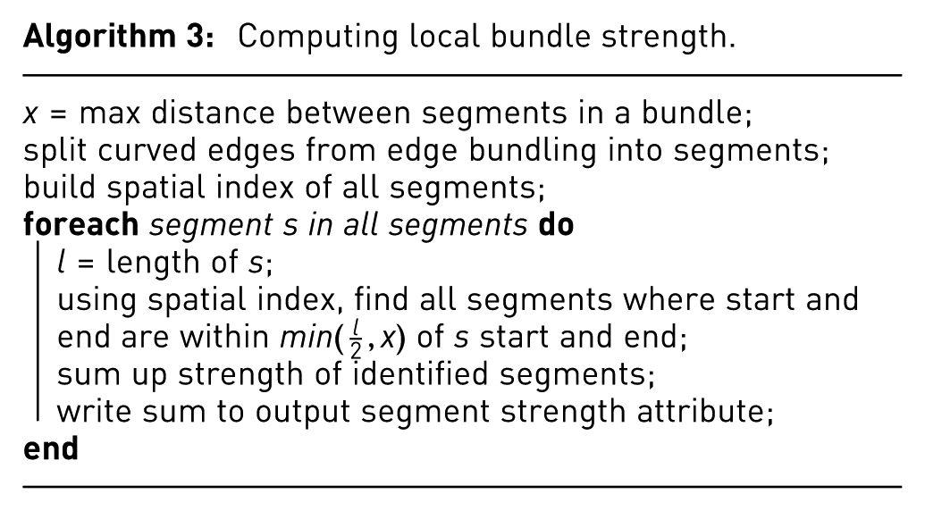
The goal of the final visualization is to convey both direction and strength of the computed edge bundles. Edge bundling alone does not provide information about the strength of a bundle at a particular location. The previous steps only modify the edge geometries by introducing control points. Edge bundling visualizations of bundle strength are usually heatmaps that represent the number of edges passing through each pixel.⁹ This is not sufficient to create an actual flow map, where line width is scaled by a local flow strength value. To compute the local strength of a bundle, we propose the following method, which is outlined in Algorithm 3: We identify edge segments that are part of the same bundle using a spatial index instead of clustering with a density-based algorithm (as suggested in Zielasko et al.¹¹), which does not provide control over the spatial extent of resulting clusters. First, we split the edges generated during edge bundling into segments that are straight lines between consecutive control points. For each segment s, we then identify all other segments that start and end at approximately the same location. To avoid merging of consecutive segments, the acceptable distance between start and end locations is half the length of s.

Algorithm 3: Computing local bundle strength.
x = max distance between segments in a bundle; split curved edges from edge bundling into segments; build spatial index of all segments; foreach segment s in all segments do l = length of s; using spatial index, find all segments where start and end are within $\min (\frac{l}{2}, x)$ of s start and end; sum up strength of identified segments; write sum to output segment strength attribute; end

Additionally, our goal is to preserve the direction of the flow. During edge bundling, all compatible edges—irrespective of directionality—are merged into one bundle if they are geometrically similar. During the visualization step, we use a GIS-based approach to offset flows with different directions: we apply a positive offset to each line that is drawn. A positive offset shifts the line to the right with respect to the flow line direction. The value of the offset scales with the local strength of the bundle to ensure that opposing flows within a bundle do not overlap each other while avoiding a gap between opposing flows. It is worth noting though that this approach cannot prevent overlaps of flows in different bundles. which we discuss in more detail in section ``Results''.

A color gradient (Viridis) from dark to light encodes the direction of the flow. This gradient has been chosen since it is colorful, perceptually uniform, and robust to colorblindness.⁴⁴ An alternative approach would be to use a gradient with reduced opacity in the center, as discussed by Boyandin et al.⁴⁵ This approach reduces occlusion since underlying flows can still be seen through the transparent flow lines. We find though that this approach makes it more difficult to follow flows from their origin to their destination and therefore decided to use a dark to light gradient (similar to the intensity-based representation in Holten et al.²⁴) instead.

Beyond gradients, edge bundling does not make it possible to use common flow map symbols with arrows (as discussed, for example, by Koylu and Guo⁴⁶) or tapered representations (as favored in Holten et al.²⁴) since bundles disband as they reach the destination locations where arrow heads would be placed or tapered lines would be widest in traditional node-based flow maps.

Finally, the bundles are sorted by their weight before drawing. Stronger bundles are drawn above weaker ones to further reduce visual clutter and emphasize strong connections.

Implementation

Our approach has been implemented for the open-source geographic information system QGIS (http://www.qgis.org). Clustering and edge bundling are implemented as Python scripts in the QGIS Processing Toolbox.¹² The source code is open and available on Github (https://github.com/dts-ait/qgis-edge-bundling). We use QGIS version 2.18 with Python version 2.7.5. For clustering, we use the k-means implementation of the machine learning library scikit-learn (http://scikit-learn.org/stable/). Figure 6 shows the QGIS Processing model used to perform edge bundling and summarization. The potential initial edge clustering step is not part of this model since it is an optional step.

Figure 6.

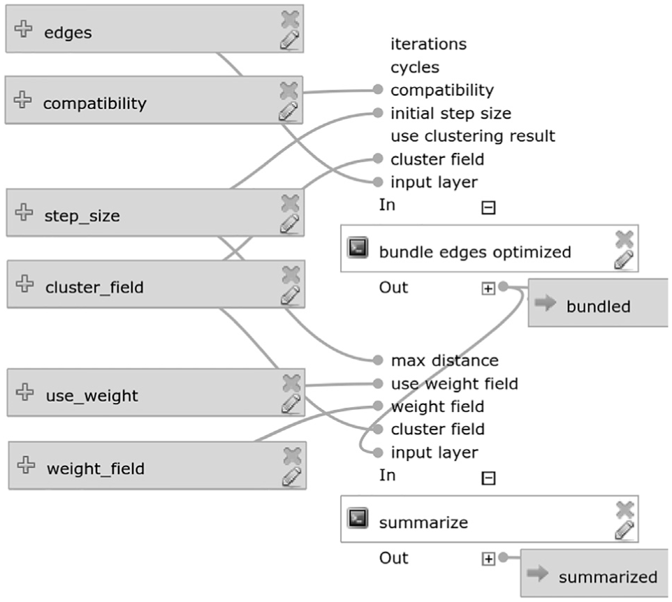
QGIS processing model. The model covers the edge bundling and the summarization step.

We have tested our implementation on both Windows and Ubuntu systems. All runtimes reported in this article were recorded for an Intel Core i7 2.9 GHz system with 16 GB of memory available, a Samsung SSD 840 EVO hard drive, and Windows 8.1 64 bit installed. The runtime of our Python implementation is listed in Table 2. The runtime for the clustering step corresponds to the time it takes to compute the optimal number of clusters as described in section “Methodology.” The runtime for the edge bundling step summarizes computing edge compatibilities, edge bundling itself, and writing the final result to disk in a GIS format. For the experiments listed in Table 2, where the compatibility threshold was set to $0.5$ , computing compatibilities consumed 48% of the edge bundling runtime for Flows Vienna and 38% of the runtime for Migration Austria. The edge compatibility is static as long as the edge configuration (i.e. the node positions) does not change. We therefore suggest to pre-compute the edge compatibility and store it in a separate file, which can be parsed before starting the edge bundling. In preliminary tests, this reduces the runtime of the edge bundling process by 30%–50%.

Table 2.

Algorithm runtime (HH:MM:SS) and the maximum memory consumption for different data sets.

Data set	# Edges	# Clusters	Clustering	Edge bundling	Summarization	Total	Max. memory
Migration Austria	72	1	–	00:00:04.76	00:00:02.52	00:00:07.28	63 MB
Gull migration	398	1	–	00:00:58.81	00:00:28.12	00:01:26.93	95 MB
Flows Vienna	1602	6	00:00:00.01	00:03:29.12	00:00:49.32	00:04:18.45	170 MB
Migration US	4009	6	00:00:03.76	00:21:07.68	00:02:33.80	00:23:45.24	254 MB
Flights Europe	15,812	131	00:00:44.32	05:33:56.57	00:23:11.84	05:57:12.73	1.6 GB

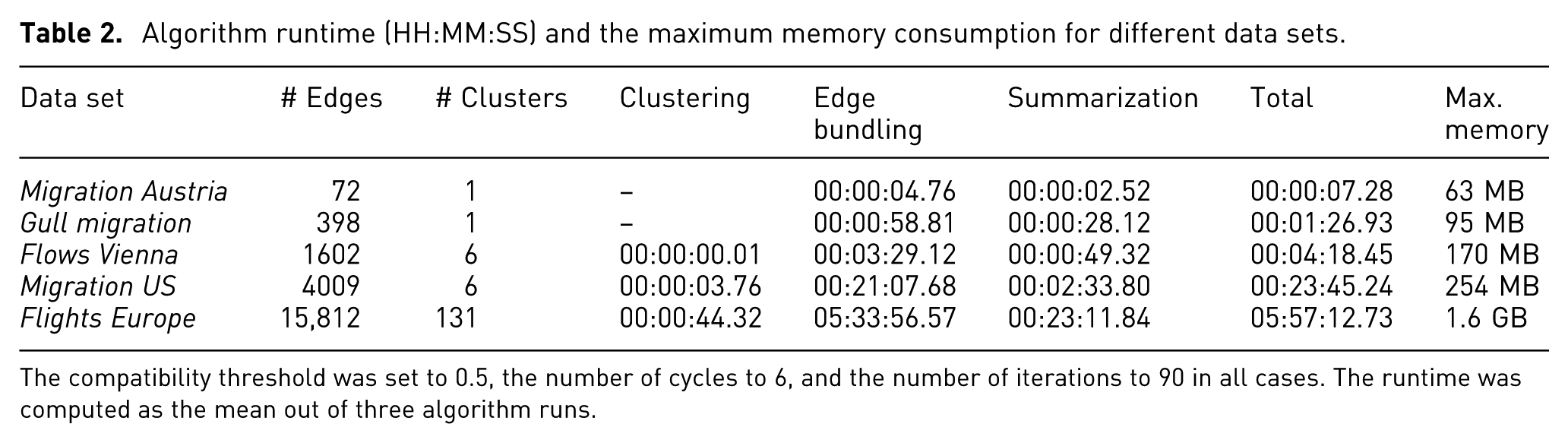
The compatibility threshold was set to $0.5$ , the number of cycles to $6$ , and the number of iterations to $90$ in all cases. The runtime was computed as the mean out of three algorithm runs.

The computational effort of the edge bundling step increases quadratically with the number of edges and is influenced by several parameters, namely the compatibility threshold, the number of cycles, and the number of iterations. If the compatibility threshold is increased, there are fewer compatible edges for bundling and the relative runtime of edge bundling will decrease. The influence of the parameters together with edge bundling results is discussed in section “Results.”

Results

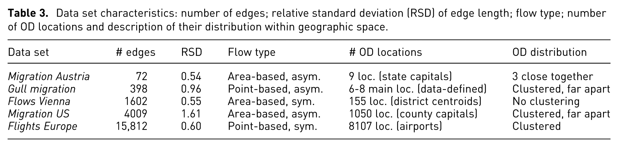
We evaluate our approach by applying it to different OD flow data sets with increasing size from $72$ to $15, 812$ edges. The data sets cover both area-based and point-based OD flow use cases, where point-based flow data are characterized by an unlimited number of potential OD locations, and area-based flow data where OD locations are limited to pre-defined areas (often represented by their area centroid). An overview of the different data set characteristics is presented in Table 3. Besides the number of edges and the type of OD flows, further data set characteristics that are worth investigation include the number of distinct OD locations as well as the distribution of OD locations. The distribution of OD locations is described using spatial point pattern analysis. Figure 7 presents an analysis of the OD point patterns using the empty-space function F and nearest-neighbor distance distribution function G.⁴⁷ (The Migration Austria data set is excluded from Figure 7 due to the low number of edges and ODs which does not allow for a useful statistical analysis.) If the empirical curve of F (solid black) is below the theoretical curve (dashed red), empty-space distances are larger than would be expected if the corresponding patterns were completely random. Therefore, this indicates clustering.⁴⁸ The interpretation of the nearest-neighbor distance distribution function G is the opposite of that for F. Accordingly, if the empirical curve (solid black) is above the theoretical curve (dashed red), distances are shorter than expected for a completely random pattern. This indicates clustering.⁴⁸

Table 3.

Data set characteristics: number of edges; relative standard deviation (RSD) of edge length; flow type; number of OD locations and description of their distribution within geographic space.

Data set	# edges	RSD	Flow type	# OD locations	OD distribution
Migration Austria	72	0.54	Area-based, asym.	9 loc. (state capitals)	3 close together
Gull migration	398	0.96	Point-based, asym.	6-8 main loc. (data-defined)	Clustered, far apart
Flows Vienna	1602	0.55	Area-based, sym.	155 loc. (district centroids)	No clustering
Migration US	4009	1.61	Area-based, asym.	1050 loc. (county capitals)	Clustered, far apart
Flights Europe	15,812	0.60	Point-based, sym.	8107 loc. (airports)	Clustered

Figure 7.

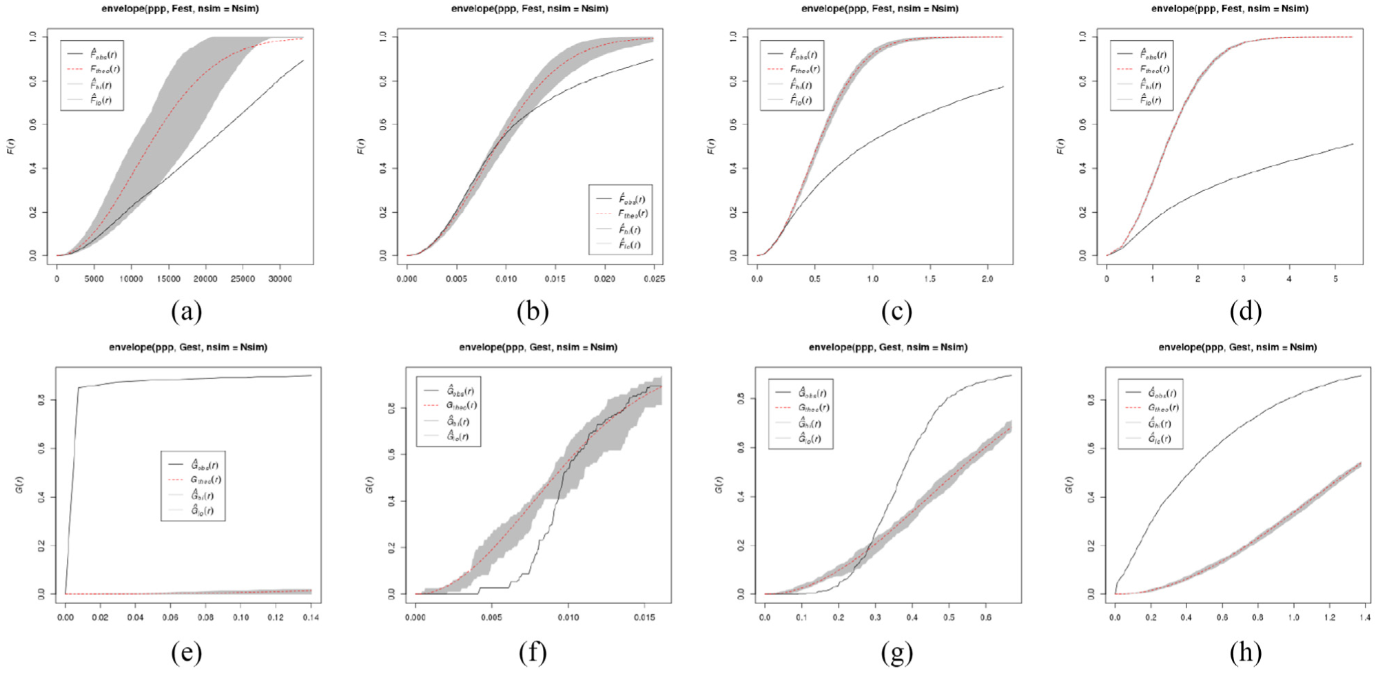
Point pattern statistics of flow origins and destinations. Empty-space function F and nearest-neighbor distance distribution function G. Empirical curve (solid black) and theoretical curve (dashed red). (Number of simulated point patterns $NSim = 10$ ). (a) F of Gull migration: potential clusters, (b) F of Flows Vienna: potential clusters, (c) F of Migration US: clusters, (d) F of Flights Europe: clusters, (e) G of Gull migration: clusters, (f) G of Flows Vienna: no clusters, (g) G of Migration US: clusters, and (h) G of Flights Europe: clusters.

Using these examples, we discuss the impact of different data set characteristics and different parameter settings on the edge bundling results. We also analyze how the optional preceding clustering step impacts results and runtime.

Migration Austria

Our smallest sample data set Migration Austria contains domestic migration flows between the nine federal states of Austria (source: Statistics Austria (http://statistik.arbeiterkammer.at/tbi2015/wanderungen.html)). It thus represents the area-based OD flow use case. For each of the 72 edges in the data set, an attribute is stored representing the number of people that moved along this edge, from one federal state to another. The raw flow data, with the width of the edges scaled by the number of movements, is shown in Figure 8. Node positions represent the location of state capitals. Since the capitals of Upper Austria (OO), Lower Austria (NO), and Vienna (WI) are aligned on an almost straight line, this raw flow data view already illustrates the issue of occlusion, since the flow between NO and WI partially covers the smaller flow between OO and WI, as well as some other flows to and from NO and WI.

Figure 8.

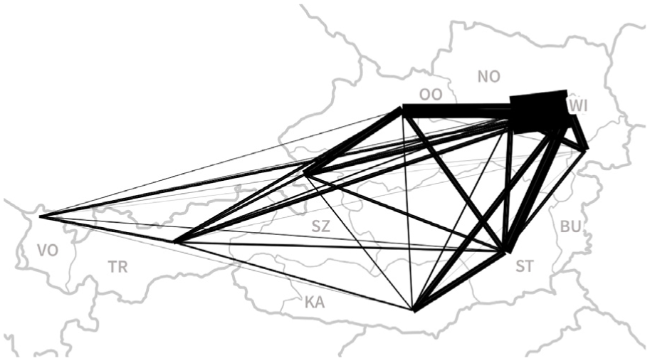
Migration Austria. This data sets consists of 72 edges. Line widths are scaled by flow strength. The largest number of movements is observed between the two federal states of Vienna (WI) and Lower Austria (NO).

Due to its small number of edges, this data set is well suited to explore the effects of different parameter settings. Edge bundling results strongly depend on the chosen parameter settings. Figures 9 and 10 show the edge bundling results for different parameter variations.

Figure 9.

Compatibility threshold parameter. The compatibility threshold ensures that only edges with a compatibility score higher than the threshold are involved in edge bundling. Direction is encoded using a dark to light gradient according to the Viridis colormap. (a) A low threshold (Compatibility = 0.45) leads to a strong bundling effect, because more edges are used. (b) An ideal parameter value for the compatibility threshold (Compatibility = 0.5) results in bundles of similar edges.(c) If the threshold is too high (Compatibility = 0.55), only few or no edges at all are considered compatible, and the bundling effect is lost. Step size = 500 m in all three examples.

Figure 10.

Step size parameter. The step size defines how strong the control points are pushed toward the calculated forces. (a) If the step size is too small (100 m), the bundling effect is hardly visible. (b) An ideal step size (1000 m) leads to nicely shaped bundles. (c) If the step size is too high (10,000 m), it may result in artifacts in the visualization as shown in more detail in Figure 11. Compatibility = 0.5 in all three examples.

The compatibility threshold parameter influences how many edges are involved in edge bundling. The effect of different parameter settings can be seen in Figure 9. The lower the compatibility threshold, the more edges are involved in the calculation, which results in stronger bundling effects, but also longer runtime. If the threshold is set to a higher value, fewer edges are included in the calculation which results in a more loosely bundled result. For example, the flow between Tirol (TR in Figure 8) and Carinthia (KA) is bundled if the compatibility threshold is set to 0.45 or 0.5 (Figure 9(a) and (b)) but is not bundled for 0.55 (Figure 9(c)). Since the threshold is a hard limit, it has to be set very carefully.

The step size parameter controls how strongly the calculated forces affect the new control point positions. In our GIS-focused implementation, the step size is set according to the distance unit used by the input data set’s coordinate reference system. In the examples presented here, step size is given in meters. The effect of the step size parameter can be seen in Figure 10. If set too low, the bundling effect is hardly visible. If set too high, the edge bundling algorithm might produce artifacts. Note that the step size is also influenced by the compatibility threshold parameter. This is due to the fact that stronger forces are applied to the control points if the compatibility threshold is lower and consequently more edges are included in the computation. Then the step size needs to be adjusted, in case artifacts occur in the visualization.

Too high step size values can quickly lead to artifacts in the bundling results. Figure 11 shows how increasing the step size excessively leads to zig-zagging edges in the bundling results. The reason for these problems is that the positions of new control points are determined based on the product of computed forces and step size. The step size is halved after every cycle. To achieve a smooth bundle with a high step size, the number of cycles therefore has to be increased accordingly, at the cost of longer computation times.

Figure 11.

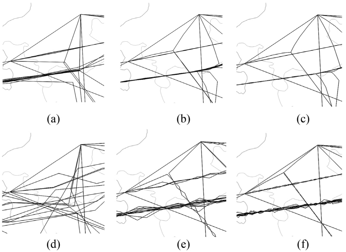
Excessive step size values cause bad bundling results, including zig-zagging edges: (a) step size = 1000 m; cycle 2, (b) step size = 1000 m; cycle 4, (c) step size = 1000 m; cycle 6, (d) step size = 10,000 m; cycle 2, (e) step size = 10,000 m; cycle 4, and (f) step size = 10,000 m; cycle 6.

For this data set, edge bundling proves efficient in bundling some flows, most notably between the north-eastern states (NO, WI, BU) which are located close to each other, and the states to the west and south (VO, TR, KA, ST). Nonetheless, the results also show that edge bundling does not address the above mentioned issue of occlusion by the big flow between NO and WI in an efficient way. The only change to the situation that can be observed is that the flow between OO and WI is attracted by the flow between OO and Burgenland (BU) and therefore ends up slightly curved toward the south. While there are approaches to extend edge bundling to push different bundles apart, these approaches would be of limited use for this kind of data set where some nodes (WI, NO, and BU in this case) are located very close together and are connected by strong flows. There is simply not enough space to resolve this issue without moving nodes or reducing line width to a point where flow strengths would be indistinguishable.

Gull Migration

The Gull Migration data set contains trajectories of lesser black-backed gulls⁴⁹ (published in the Movebank Data Repository⁵⁰). This data set represents an example of point-based flows and covers multiple years (from 2009 until 2015). Every edge represents one bird’s movement; therefore, the edges do not have an additional weight attribute. The published original GPS trajectories are split at stops of more than 7 days. Subtrajectories shorter than 100 km are removed. This distance limit is in agreement with the original paper by Wikelski et al.,⁴⁹ where 100 km is the threshold between local and migratory trips. The final 398 OD flows (depicted in Figure 12(a)) are generated by extracting subtrajectory start and end locations.

Figure 12.

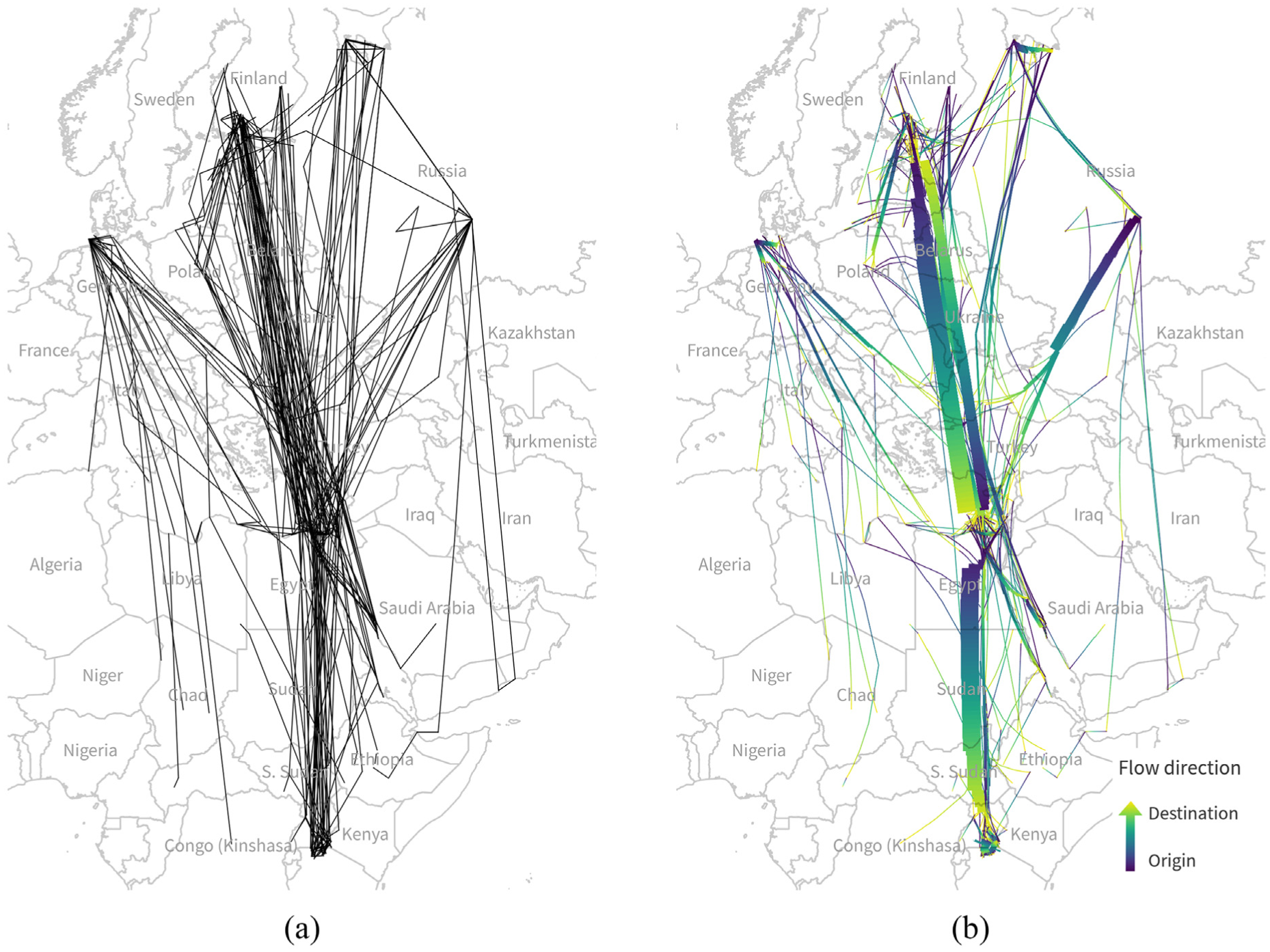
Gull migration. Point-based flows where each edge represents one bird’s movement: (a) original GPS trajectories were converted to 398 OD flows by connecting consecutive stops of more than 7 days as well as trajectory start and end locations and (b) bundled gull migration edges with a compatibility threshold of 0.55 and step size of 0.01°. Direction is encoded using a dark to light gradient according to the Viridis colormap.

The number of main OD locations, that is, locations where many flows originate or end, is subject to interpretation. It depends on the chosen threshold for the minimum number of flows that are considered necessary for a main OD location. Notable locations with multiple flows include southern Finland, Heligoland (north-western Germany), the southern coast of the White Sea and Kazan in Russia, the eastern Mediterranean, the Nile Delta, and Lake Victoria. In any case, these locations are clearly distinct and far apart.

For this data set, edge bundling succeeds in bundling flows between the main OD locations. The edge bundling results correspond well with the description of main migration routes in the original paper.⁴⁹Figure 12(b) shows that most tracked birds migrate from the north to the Nile Delta and on to Lake Victoria. It is noteworthy that the data show that most birds or their trackers do not return from Lake Victoria while there is an opposite flow back to the north from the Nile Delta. This information about movement directions is not readily discernible in the initial map of OD flows in Figure 12(a).

Looking at the bundling details, flows originating at Kazan (Russia) are largely bundled since most of them target the eastern Mediterranean or the Nile Delta. Flows from Heligoland (Germany), on the other hand, remain largely unbundled due to the wide spread of target destinations. To achieve more bundling, the compatibility threshold can be decreased as discussed for the Migration Austria data set in Figure 9.

Flows Vienna

The Flows Vienna data set contains flows between registration districts in Vienna, Austria. The data are based on trajectories derived from cell phone network data⁵¹ and comprises 1602 edges. Each edge represents at least 50 people movements. For every edge, the number of people moving along this path is stored. This data set thus represents another example of area-based OD flow data. In Figure 13(a), the raw data are shown, with line widths adjusted to the number of recorded movements along the corresponding edge. The area in the north-east of the city is separated from the more densely populated center by the Danube river. This is reflected by the limited connectivity between the two parts.

Figure 13.

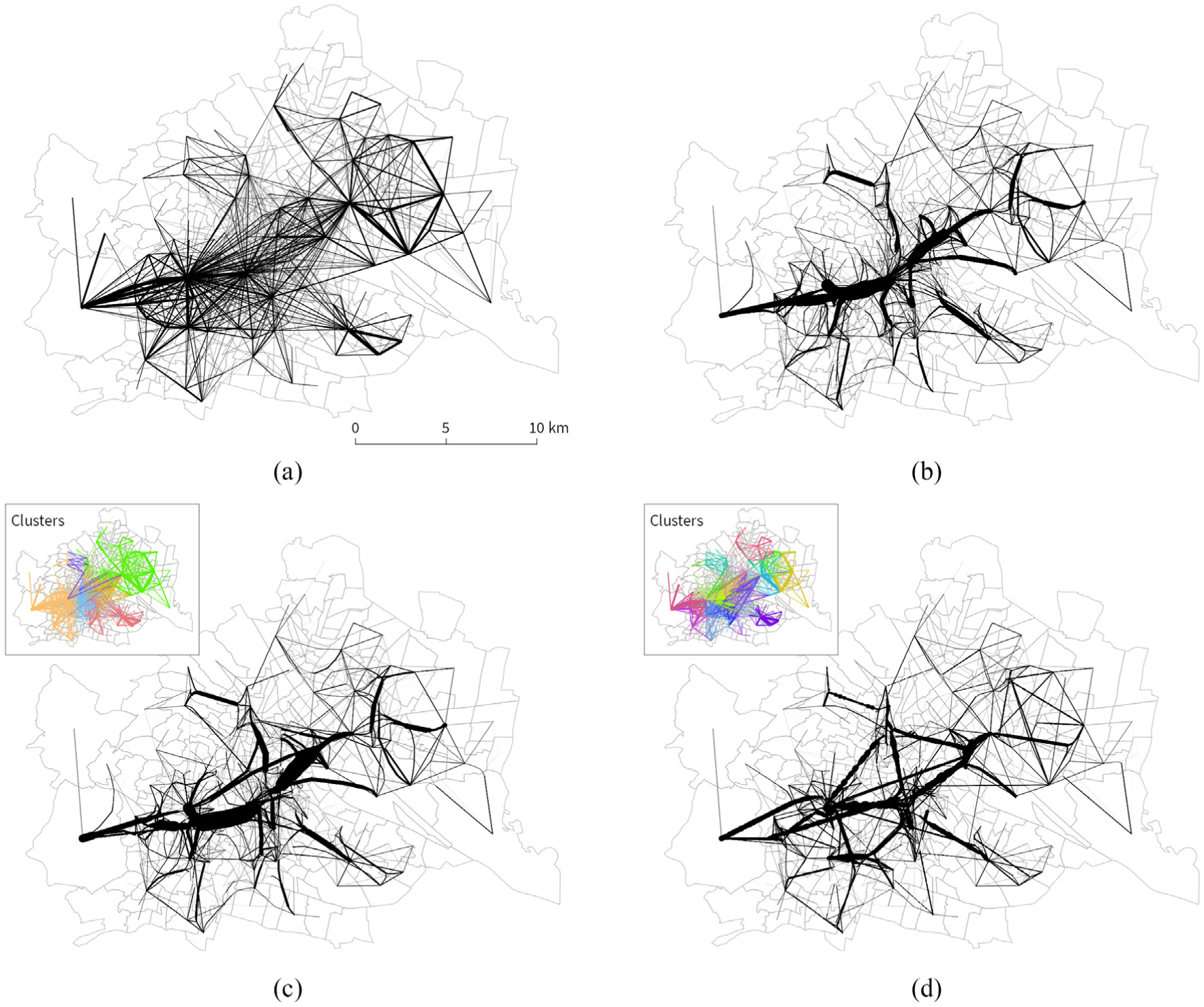
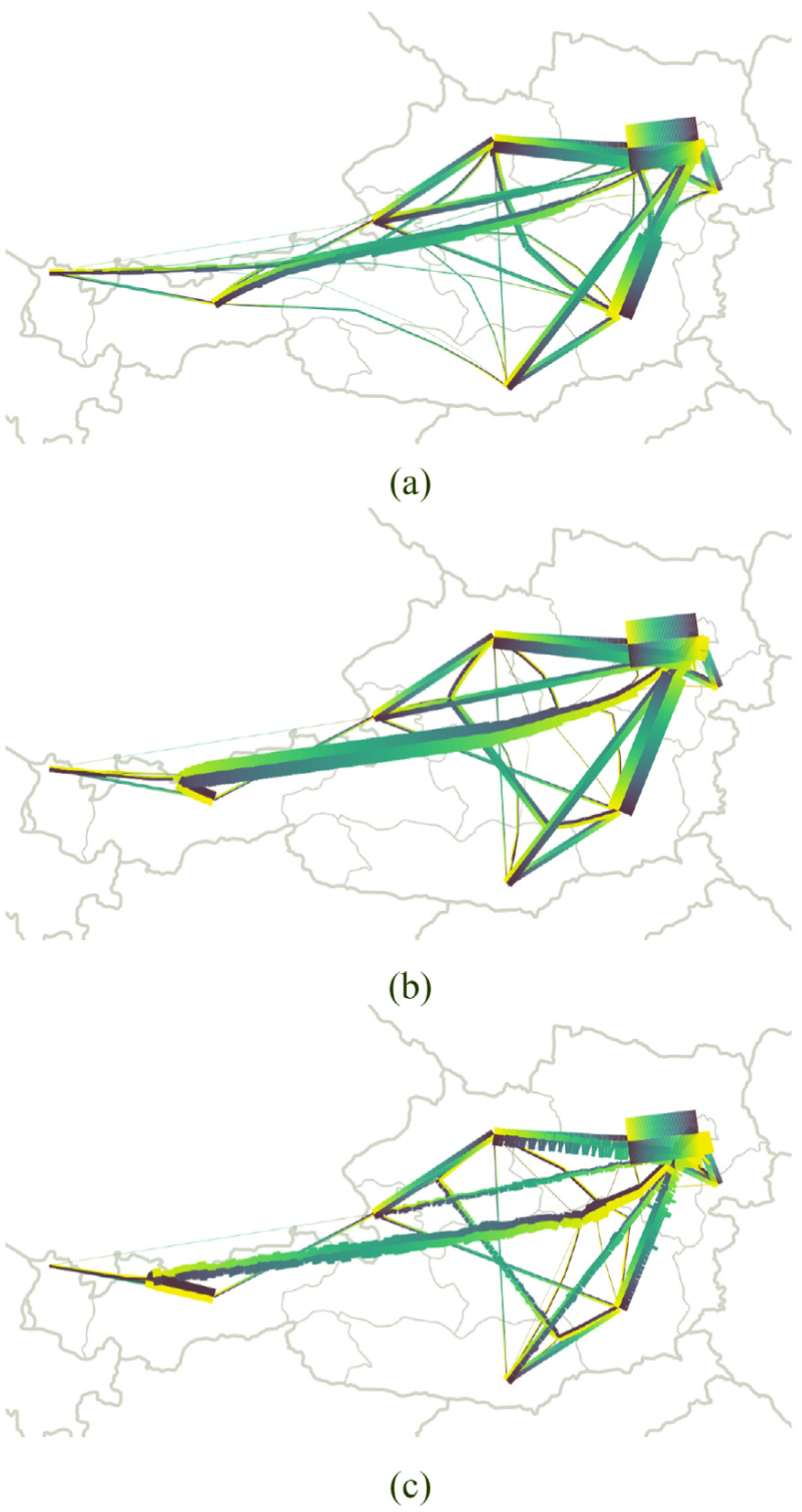
Edge clustering effect for Flows Vienna. We compare edge bundling of raw unclustered and clustered edges. Line widths are scaled by flow strength. Color-coded clusters are shown in map insets using randomly assigned colors. (a) Raw data (1602 edges). (b) Edge bundling without preceding clustering step involves all edges in the calculation (run time: 06:44.32). (c) Edge bundling based on 6 clusters (resulting from a target cluster size of 10 km) yields similar results (run time: 03:29.12). (d) In case many clusters are created (here, a target size of 5 km results in 32 clusters), compatible edges are missed which leads to different local bundling effects. (run time: 02:30.03)

In contrast to the Gull Migration example, a statistical analysis of the OD distribution in the Flows Vienna example (see Figure 7(b) and 7(f)) does not indicate clustering of OD locations. There are no clearly spatially separated main OD locations in the Flows Vienna data. Instead, there are many edges crossing at all different angles.

Figure 13(b) shows the bundling results for compatibility threshold of 0.5 and step size of 10 m. The main flow directions toward the city center (most notably: from the west, north, north-east, and south-east) have emerged as clear strong bundles. We decided against rendering flow directions using a gradient in this case since the flows are symmetrical and thus, no additional insight can be gained.

To reduce the runtime of the edge bundling algorithm, we apply our edge clustering algorithm to this data set. The original runtime of 06:44 min for the whole data set can be reduced to 03:29 min (for 6 clusters) and 02:30 min (for 32 clusters). Since edge bundling only takes place within a cluster, edge bundling results from clustered data can look different than edge bundling results from raw unclustered data. If the number of clusters is too high, compatible edges may be assigned to different clusters and therefore will not be bundled in the final visualization. An example for this can be seen in Figure 13(b)–(d), where edge bundling results based on all edges are compared to edge bundling based on clustered edges. The dominant bundles between the city center and the western and north-eastern areas in the unclustered results (Figure 13(b)) are split into an increasing number of smaller bundles in the 6 and 32 cluster results (Figure 13(c) and (d)). On the other hand, smaller bundles in the north-west and south-east remain largely unaffected by clustering. This can be explained by the fact that in these areas, our clustering did a good job at anticipating edge compatibilities.

Migration US

The Migration US data set contains flows between capital cities of counties in the United States. The data have been calculated from the census in 2000 (source: United States Census Bureau (https://www.census.gov/population/www/cen2000/ctytoctyflow/)). Each edge represents a flow of at least 1000 people, resulting in 4009 edges between 1050 OD locations.

The edges in this data set show the by far highest relative standard deviation of edge length values (see Table 3) indicating that the data set contains a mix of very short and very long edges with few medium length edges. A statistical analysis of OD distributions in this example (Figure 7(c) and (g)) indicates that OD locations are clustered. This finding is confirmed by visual interpretation of the map of OD flows in Figure 14(a) and comparison with the Vienna Flows example in Figure 13(a) where ODs are not clustered.

Figure 14.

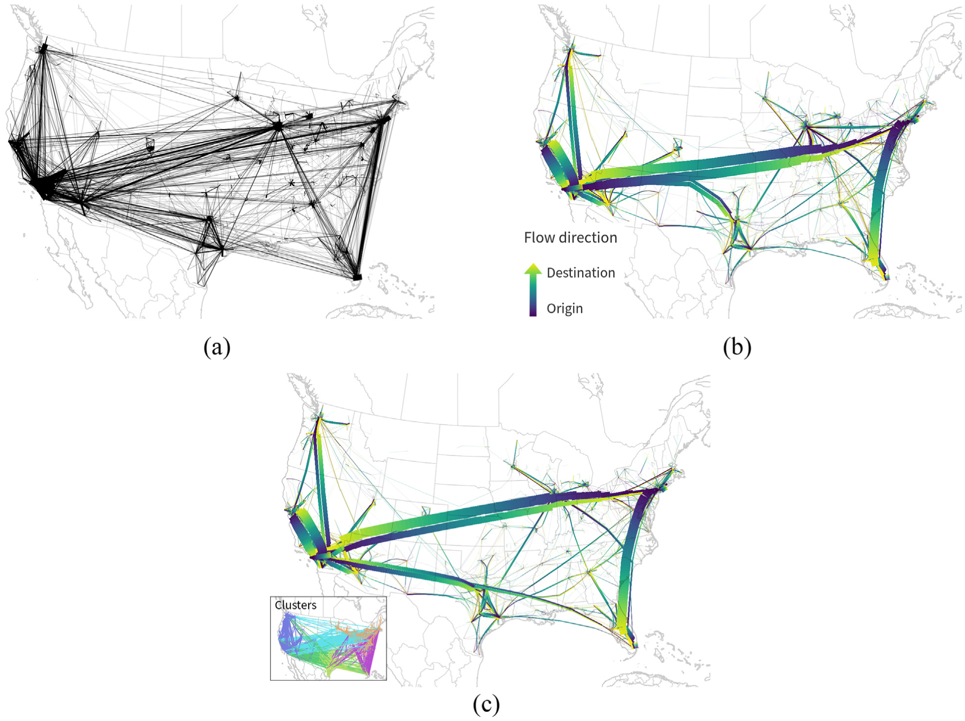
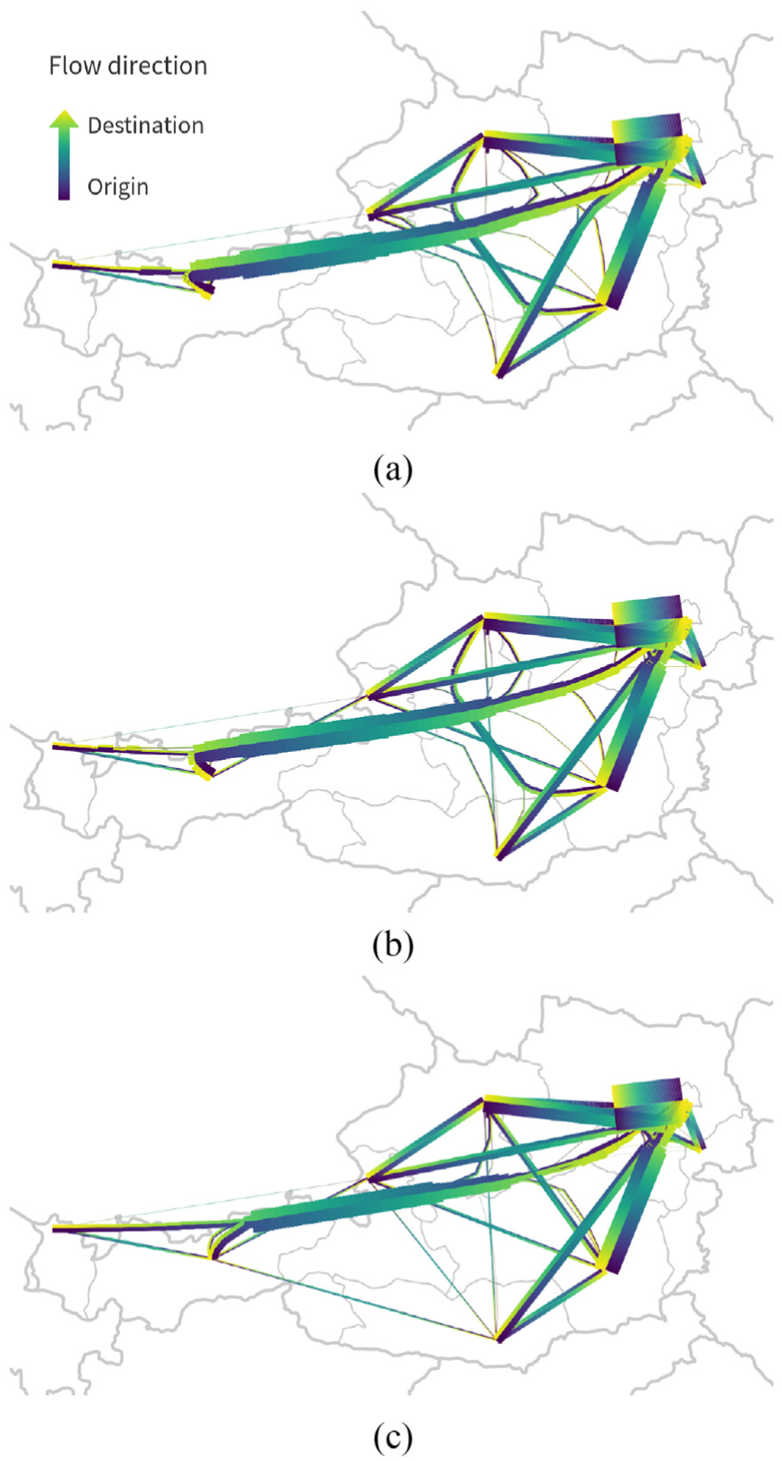
Edge clustering effect for Migration US data set major migration flows of at least 1000 people in the US with 4009 edges between 1050 OD locations. Line width are scaled be flow strength. Color-coded clusters are shown in map insets using randomly assigned colors. Direction of bundles is encoded using a dark to light gradient according to the Viridis colormap. (a) Raw data. (b) Edge bundling without preceding clustering step (run time: 38:71.12). (c) Edge bundling after clustering with a target size of 1000 km resulting in six edge clusters most notably splits the bundle between California and Texas from the bundle between California and the North-east (run time: 23:45.24).

Edge bundling results in Figure 14(b) and (c) show strong migration flows along the West coast, between California and Texas, between California and the North-east, and from the North-east to Florida. Similar to the Gull Migration example, this example also succeeds in communicating flow direction since the asymmetry of flows between the North-east and Florida is very well visible.

The majority of bundles remain stable between the unclustered (Figure 14(b)) and clustered solution (Figure 14(c)). Clustering the edges in this example most notably splits the bundle between California and Texas/Florida from the bundle between California and the North-east. This results in slightly different geographic locations for these bundles. In the clustered solution, the California to North-east bundle ends up in a position that overlaps Denver and Chicago.

Even though the Migration US data set contains more than twice as many edges than the Flows Vienna data set, the results appear no more visually cluttered and maybe even less cluttered. Our hypothesis—which will require further testing in the future—therefore is that edge bundling produces better results for flow data sets with spatially clearly separated clusters of OD locations. Furthermore, we expect better edge bundling results for data sets with spatial line patterns that indicate flow edge clustering.

Flights Europe

Our largest data set Flights Europe consists of OD flow data describing flight connections between European airports (source: OpenFlights (https://github.com/jpatokal/openflights/tree/master/data)). This data set represents point-based OD flows and contains 15,812 edges. Every edge represents one flight connection; therefore, the edges do not have an additional weight attribute. Raw data and edge bundling results are shown in Figure 1. Similar to the Flows Vienna example, flight flows are symmetrical and therefore, rendering direction using a gradient does not provide further insight.

To divide this edge bundling problem into manageable pieces, we chose a target cluster size of 1000 km which resulted in 112 edge clusters. In densely populated areas, one-point cluster encompasses multiple busy airports. For example, Amsterdam, Brussels, Frankfurt, and Berlin are all part of the same point cluster. Figure 15 shows the results. Dominant edge bundles highlight major connections between the United Kingdom, central and southern Europe. Some areas, such as the eastern part of the Iberian peninsula around Barcelona, or south-eastern Europe between Athens and Istanbul, show multiple strong connections to the rest of the continent without any dominant bundle.

Figure 15.

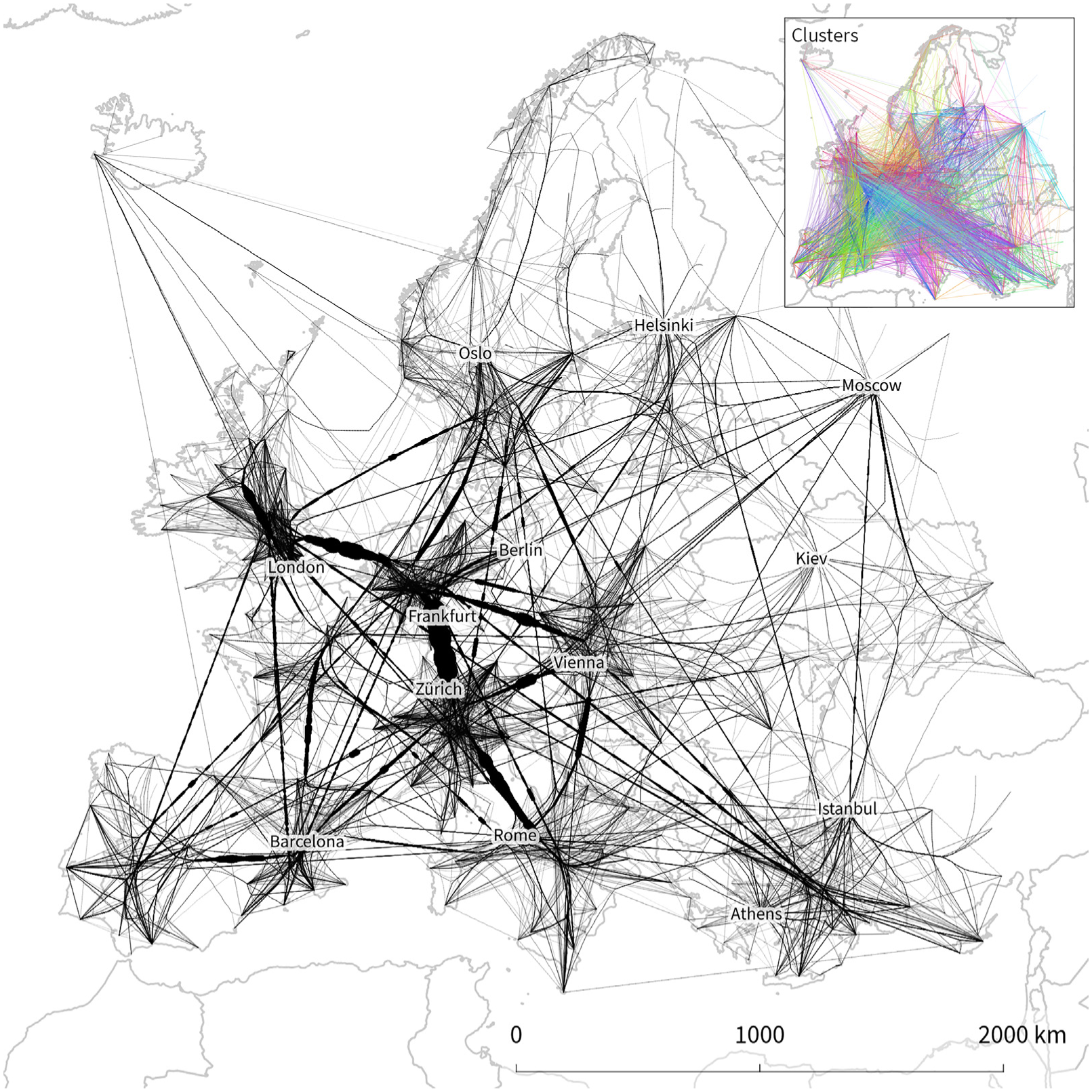
Bundling results for target cluster size of 1000 km resulting in 112 edge clusters (comp = 0.5, step size = 1000 m, cycles = 5, iterations = 90). Color-coded edge clusters are shown in the map inset using randomly assigned colors.

Edge patterns in central Europe resemble patterns found in Figure 13(d). It is therefore reasonable to assume that edge bundling the unclustered data set would lead to a stronger bundling effect. Due to the size of this problem, this is currently intractable.

To gain a better understanding of our edge bundling results, we compare them to OD maps as proposed by Wood et al.⁵ and shown in Figure 16. Locations such as Keflavik and Moscow stand out in both maps since they are surrounded by mostly empty space. While regions in the edge bundling map are result of the data-driven clustering of OD locations, OD maps employ a regular grid to subdivide space. Thus, neither approach enables the reader to identify individual connections between specific airports. Consequently, the interpretation is limited to connectivity between regions. Nonetheless, compared to maps of raw OD flows (Figure 1), edge bundling and OD maps enable the reader to determine regions connected by strong flows as well as weakly connected regions. While edge bundling provides an intuitive global overview, it “trades clutter for overdraw.”¹⁸ OD maps, on the other hand, enable focused analysis of individual cells by reducing occlusions. In particular, OD maps manage to communicate the number of local flows within a cell, which are often covered up in edge bundling visualizations.

Figure 16.

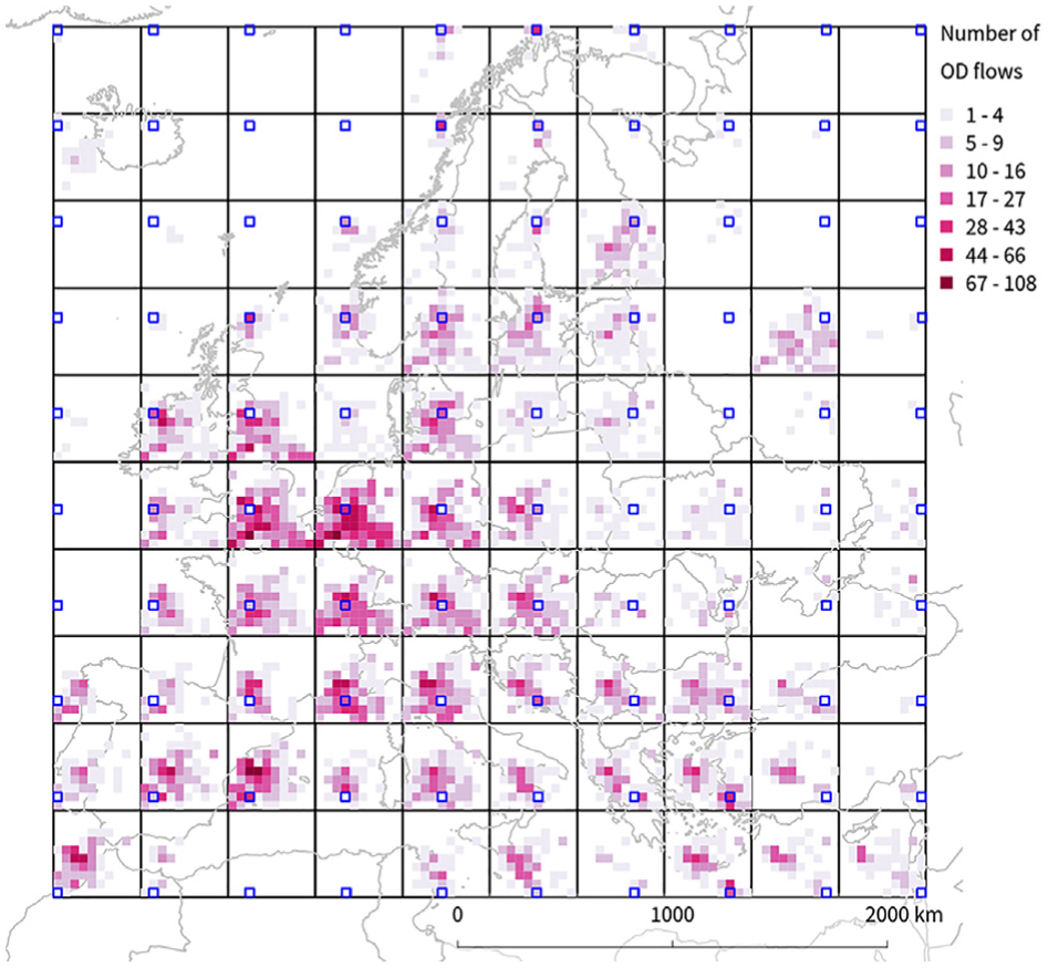
Alternative visualization of the Flight Europe data set using the OD map method described by Wood et al.⁵ Classes are assigned using Jenks natural breaks classification. Cells with zero flights were excluded from the classification.

Conclusion and future work

User-friendly open-source GIS provide spatial data analysis and visualization functionality to a wider audience than previous proprietary GIS offerings. To date, both proprietary and open-source GIS tend to draw geometry data as is. One notable exception are point cluster renderers that help to dissolve overlapping points by aggregating them in composite symbols. Beyond point cluster renderers, there are no equivalent GIS solutions for line data sets. Common techniques from the information visualization community, such as edge bundling and force-directed layouts, have not been implemented so far. However, adding appropriate tools to handle line data sets is an important step from the naive “paint by numbers” critique that GIS often face and increase GIS capabilities to create outputs that involve transformation to represent data clearly and effectively.

We explored the applicability of edge bundling to spatial data sets and necessary adaptations under the constraints inherent to platform-independent GIS scripting environments. Our approach includes a new clustering technique, edge bundling using matrix computation, spatial indexes to determine local bundle strength, and avoiding overlap using offsets during rendering.

To speed up computations, we presented a clustering method that ensures within-cluster consistency. The optimal number of clusters is determined automatically based on a user-specified maximum target cluster size. Our approach enables GIS visualizations of flow strength and direction. We determine locale bundle strength using spatial indexes. To avoid overlaps of opposing flows, we leverage line offsets during rendering. Flow direction is communicated using gradients. To provide edge bundling capabilities for a wide audience, our edge bundling algorithm is optimized to run within platform-independent GIS scripting environments.

Flow maps should fulfill (among others) the following requirements:⁵ (1) Be able to visually represent a large number of OD flows and OD locations, (2) Preserve the spatial configuration of the study area, (3) Be able to distinguish between origin and destination of a flow, (4) Be able to compare opposite directed flows (OD- vs DO-flows), and (5) Be able to distinguish artifacts of the visualization from characteristics of the data under investigation. The results in this article show that the visualizations created with edge bundling fulfill many of these common requirements. Edge bundling provides an overview of the current situation (1) and preserves the spatial configuration of the study area (2). In most cases, it is possible to distinguish between origin and destination of a flow (3). There are, however, cases where flow maps are required to emphasize the representations of the OD locations over the geometry of the paths that link them.⁵ In this case, edge bundling is not a good choice, since it de-emphasizes individual OD locations while putting emphasis on strong bundles. Since we used gradients and line offsets to encode direction, it is still possible to distinguish between opposite directed flows (4). Beyond gradients, edge bundling does not make it possible to use common flow map symbols with arrows since bundles disband as they reach the destination locations where arrow heads would be placed in traditional node-based flow maps. Nonetheless, it is worth noting that the type of edge bundling we implemented does not manage to resolve all cases of occlusion. Skeleton-based edge bundling approaches²⁵ would likely be a better choice if this is a high priority for the visualization but this method comes with its own disadvantages. Finally, edge bundling helps to reduce clutter¹⁸ in the visualization and can reveal patterns which would not be visible otherwise (5). It is very important, though, to adjust the parameters to the current data set, to avoid artifacts such as bad bundling and zig-zagging edges in the visualization. Other artifacts result from the clustering step, since edges are only bundled within clusters. Furthermore, edge bundling methods can wrongly emphasize random noise if the input data set does not contain any salient structures.⁵²

To evaluate our approach in different contexts, we provide a wide range of different real-world spatial flow data set examples. We looked into the type of flow (area-based or point-based), number and distribution of OD locations, as well as number of edges and edge length distribution. So far, it remains unclear which data set key characteristics determine whether a spatial flow data set can be edge bundled efficiently. One beneficial characteristic seems to be spatially clearly separated clusters of OD locations. More work is needed, for example, concerning statistics for spatial line patterns and their effect on edge bundling results.

So far, our implementation does not consider edge weights during edge bundling. For future work, we therefore plan to implement a weighted edge bundling approach.¹⁰ We also plan to explore the possibility to automatically extract ideal parameter values from the data. Since edge bundling for large data sets can take minutes, a trial-and-error approach for finding the right parameter values can be cumbersome. There are already existing approaches on the visual analysis of parameter spaces,⁵³ and it would be helpful to apply such approaches.

The speed of our implementation stands to gain from planned parallelization support in the QGIS geoprocessing framework. If one were to abandon the goal of providing a tool that runs on all platforms, another option to increase performance would be to leverage GPU computing power, for example, using PyCUDA. This would, however, limit the tool to be used on PCs with Nvidia GPU. To avoid this vendor lock-in, the open-standard OpenCL could provide a viable alternative. Furthermore, the performance of the edge bundling algorithm can be improved by pre-calculating the compatibility of the input edges. As explained in section “Implementation,” the compatibility calculation constitutes a major part of the overall edge bundling runtime. Since compatibility values do not change as long as the edges remain the same, it is not necessary to repeat compatibility calculations for each edge bundling run. We therefore plan to decouple the compatibility calculation and to store the data externally. Another potential venue to improve performance is feature reduction. Since each individual OD flow is split into multiple segments, the number of features in the final visualization is many times higher than the number of input features. In the future, we envision an additional feature reduction step before, during, or after the summarization step.

Finally, in the current implementation, there is no mechanism to avoid different bundles overlapping OD locations or other bundles. This can limit readability and hide patterns. We expect that it will be a very interesting and challenging task to find suitable techniques to efficiently handle overlapping bundles in the visualization by improving on Buchin et al.’s²⁸ spiral trees or other novel approaches.

Footnotes

Acknowledgements

The authors would like to thank all researchers who provided flow data sets used in this article: Wikelski et al.⁵⁰ for the Gull Migration data set, Sugar et al. (https://github.com/upphiminn/d3.ForceBundle/blob/master/example/bundling_data/migrations.xml) for the US Migration data set, and Patokallio for the OpenFlights data set. The Vienna Flows data set is based on trajectories derived from mobile network data which has been collected within the SEMAPHORE project at AIT ().

References

Andrienko

Fuchs

et al> . Revealing patterns and trends of mass mobility through spatial and temporal abstraction of origin-destination movement data. IEEE T Vis Comput Gr 2017; 23: 2120–2136.

Ellis

Dix

. A taxonomy of clutter reduction for information visualisation. IEEE T Vis Comput Gr 2007; 13(6): 1216–1223.

Schaeffer

. Survey: graph clustering. Comput Sci Rev 2007; 1(1): 27–64.

Elmqvist

Goodell

et al . ZAME: interactive large-scale graph visualization. In: Proceedings of the IEEE Pacific visualization symposium (PacificVis ’08), Kyoto, Japan, 5–7 March 2008, pp. 215–222. New York: IEEE Computer Society.

Wood

Dykes

Slingsby

. Visualisation of origins, destinations and flows with OD maps. Cartogr J 2010; 47(2): 117–129.

Burch

Vehlow

Konevtsova

et al . Evaluating partially drawn links for directed graph edges. In: Proceedings of the 19th international conference on graph drawing (GD ’11), Eindhoven, 21–23 September 2011, pp. 226–237. Berlin; Heidelberg: Springer-Verlag.

Cui

Zhou

et al . Geometry-based edge clustering for graph visualization. IEEE T Vis Comput Gr 2008; 14(6): 1277–1284.

Holten

. Hierarchical edge bundles: visualization of adjacency relations in hierarchical data. IEEE T Vis Comput Gr 2006; 12(5): 741–748.

Holten

Van Wijk

. Force-directed edge bundling for graph visualization. Comput Graph Forum 2009; 28(3): 983–998.

10.

Selassie

Heller

Heer

. Divided edge bundling for directional network data. IEEE T Vis Comput Gr 2011; 17(12): 2354–2363.

11.

Zielasko

Weyers

Hentschel

et al . Interactive 3D force-directed edge bundling. Comput Graph Forum 2016; 35(3): 51–60.

12.

Graser

Olaya

. Processing: a Python framework for the seamless integration of geoprocessing tools in QGIS. ISPRS Int J Geo-Inf 2015; 4(4): 2219–2245.

13.

Schumann

Tominski

. Analytical, visual and interactive concepts for geo-visual analytics. J Visual Lang Comput 2011; 22(4): 257–267.

14.

Lhuillier

Hurter

. Bundling, graph simplification trough visual aggregation: existing techniques and challenges. In: Proceedings of the 27th conference on L’interaction Homme-machine (IHM ’15), Toulouse, 27–30 October 2015, pp. 10-1–10-10. New York: ACM.

15.

Guo

Zhu

. Origin-destination flow data smoothing and mapping. IEEE T Vis Comput Gr 2014; 20(12): 2043–2052.

16.

Liang

Wang

et al . Exploring OD patterns of interested region based on taxi trajectories. J Visual 2016; 19: 811–821.

17.

Zhou

Yuan

et al . Edge bundling in information visualization. Tsinghua Sci Technol 2013; 18(2): 145–156.

18.

Lhuillier

Hurter

Telea

. State of the art in edge and trail bundling techniques. In: Proceedings of the 19th Eurographics conference on visualization—STARs (EuroVis ’17), Barcelona, 12–16 June 2017. Barcelona: Eurographics.

19.

Lambert

Bourqui

Auber

. Winding roads: routing edges into bundles. Comput Graph Forum 2010; 29(3): 853–862.

20.

Gansner

North

et al . Multilevel agglomerative edge bundling for visualizing large graphs. In: Proceedings of the IEEE Pacific visualization symposium (PacificVis ’11), Hong Kong, China, 1–4 March 2011, pp. 187–194. New York: IEEE Computer Society.

21.

Bourqui

Ienco

Sallaberry

et al . Multilayer graph edge bundling. In: Proceedings of the IEEE Pacific visualization symposium (PacificVis ’16), Taipei, Taiwan, 19–22 April 2016, pp. 184–188. New York: IEEE Computer Society.

22.

Cornel

Konev

Sadransky

et al . Composite flow maps. Comput Graph Forum 2016; 35(3): 461–470.

23.

Pupyrev

Nachmanson

Bereg

et al . Edge routing with ordered bundles. In: Proceedings of the 19th international symposium on graph drawing, Eindhoven, 21–23 September 2011, pp. 136–147. Berlin; Heidelberg: Springer.

24.

Holten

Isenberg

van Wijk

et al . An extended evaluation of the readability of tapered, animated, and textured directed-edge representations in node-link graphs. In: Proceedings of the IEEE Pacific visualization symposium (PacificVis ’11), Hong Kong, China, 1–4 March 2011, pp. 195–202. New York: IEEE Computer Society.

25.

Ersoy

Hurter

Paulovich

et al . Skeleton-based edge bundling for graph visualization. IEEE T Vis Comput Gr 2011; 17(12): 2364–2373.

26.

Luo

Liu

Chen

et al . Ambiguity-free edge-bundling for interactive graph visualization. IEEE T Vis Comput Gr 2012; 18(5): 810–821.

27.

Bach

Riche

Hurter

et al . Towards unambiguous edge bundling: investigating confluent drawings for network visualization. IEEE T Vis Comput Gr 2017; 23(1): 541–550.

28.

Buchin

Speckmann

Verbeek

. Flow map layout via spiral trees. IEEE T Vis Comput Gr 2011; 17(12): 2536–2544.

29.

Buchin

Speckmann

Verbeek

. Angle-restricted steiner arborescences for flow map layout. Algorithmica 2015; 72(2): 656–685.

30.

Kostitsyna

Speckmann

Verbeek

. Non-crossing drawings of multiple geometric Steiner arborescences. In: Proceedings of the 33rd European workshop on computational geometry (EuroCG ’17), Malmo, 5–7 April 2017, pp. 133–136. Berlin; Heidelberg: Springer-Verlag.

31.

Hurter

Telea

Ersoy

. MoleView: an attribute and structure-based semantic lens for large element-based plots. IEEE T Vis Comput Gr 2011; 17(12): 2600–2609.

32.

Van der Zwan

Codreanu

Telea

. CUBu: universal real-time bundling for large graphs. IEEE T Vis Comput Gr 2016; 22(12): 2550–2563.

33.

. Texture-based edge bundling: a web-based approach for interactively visualizing large graphs In: Proceedings of the IEEE international conference on big data (Big Data ’15), Santa Clara, CA, 29 October–1 November 2015, pp. 2501–2508. New York: IEEE Computer Society.

34.

Telea

Ersoy

. Image-based edge bundles: simplified visualization of large graphs. In: Proceedings of the 12th Eurographics/IEEE—VGTC conference on visualization (EuroVis ’10), Bordeaux, 9–11 June 2010, pp. 843–852. Chichester: The Eurographics Association.

35.

Peysakhovich

Hurter

Telea

. Attribute-driven edge bundling for general graphs with applications in trail analysis. In: Proceedings of the IEEE Pacific visualization symposium (PacificVis ’15), Hangzhou, China, 14–17 April 2015, pp. 136–147. New York: IEEE Computer Society.

36.

Han

Kamber

Tung

. Spatial clustering methods in data mining: a survey. In: Miller

Han

(eds) Geographic data mining and knowledge discovery. London: Taylor & Francis, 2001, pp. 201–231.

37.

Varghese

Unnikrishnan

Poulose Jacob

. Spatial clustering algorithms—an overview. Asian J Comput Sci Inform Technol 2013; 3(1): 1–8.

38.

Yuan

Sun

Zhao

et al . A review of moving object trajectory clustering algorithms. Artif Intell Rev 2017; 47: 123–144.

39.

Zheng

. Trajectory data mining: an overview. ACM T Intel Syst Tec 2015; 6: 29.

40.

Ferreira

Klosowski

Scheidegger

et al . Vector field k-means: clustering trajectories by fitting multiple vector fields. Comput Graph Forum 2013; 32(3): 201–210.

41.

Bouts

Speckmann

. Clustered edge routing. In: Proceedings of the IEEE Pacific visualization symposium (PacificVis ’15), Hangzhou, China, 14–17 April 2015, pp. 55–62. New York: IEEE Computer Society.

42.

Wunsch

. Survey of clustering algorithms. IEEE T Neural Networ 2005; 16(3): 645–678.

43.

Ester

Kriegel

Sander

et al . A density-based algorithm for discovering clusters in large spatial databases with noise. In: Proceedings of the 2nd international conference on knowledge discovery and data mining (KDD ’96), Portland, OR, 2–4 August 1996, pp. 226–231. Palo Alto, CA: AAAI Press.

44.

Van der Walt

Smith

. mpl colormaps, 2015, http://bids.github.io/colormap/

45.

Boyandin

Bertini

Lalanne

. Using flow maps to explore migrations over time. In: Proceedings of the geospatial visual analytics workshop in conjunction with the 13th AGILE international conference on geographic information science, vol. 2, Guimaraes, 11–14 May 2010.

46.

Koylu

Guo

. Design and evaluation of line symbolizations for origin–destination flow maps. Inform Visual 2017; 16: 309–331.

47.

Diggle

. Statistical analysis of spatial point patterns. London: Academic Press, 1983.

48.

Baddeley

Rubak

Turner

. Spatial point patterns: methodology and applications with R. Boca Raton, FL: CRC Press, 2015.

49.

Wikelski

Arriero

Gagliardo

et al . True navigation in migrating gulls requires intact olfactory nerves. Sci Rep 2015; 5: 17061.

50.

Wikelski

Arriero

Gagliardo

et al . Data from: True navigation in migrating gulls requires intact olfactory nerves. Movebank Data Repository, 2015, https://www.datarepository.movebank.org/handle/10255/move.494

51.

Widhalm

Yang

Ulm

et al . Discovering urban activity patterns in cell phone data. Transportation 2015; 42(4): 597–623.

52.

Hurter

Ersoy

Telea

. Graph bundling by kernel density estimation. Comput Graph Forum 2012; 31: 865–874.

53.

Sedlmair

Heinzl

Bruckner

et al . Visual parameter space analysis: a conceptual framework. IEEE T Vis Comput Gr 2014; 20(12): 2161–2170.