
Abstract
This paper describes a new automatic layout algorithm named CoSEP for compound graphs with port constraints. The algorithm works by extending the physical model of a previous algorithm named CoSE by defining additional force types and heuristics for constraining edges to connect to certain user-defined locations on end nodes. Similar to its predecessor, CoSEP also accounts for non-uniform node dimensions and arbitrary levels of nesting via compound nodes. Our experiments show that CoSEP significantly improves the quality of the layouts for compound graphs with port constraints with respect to commonly accepted graph drawing criteria while running reasonably fast, suitable for use in interactive applications for small to medium-sized (up to 500 nodes) graphs. A complete JavaScript implementation of CoSEP as a Cytoscape.js extension along with a demo page is freely available at https://github.com/iVis-at-Bilkent/cytoscape.js-cosep.
Keywords
Introduction
Understanding complex relations among various objects is a key recurring necessity for effective analysis and discovery in numerous domains from biological pathways to financial transaction graphs to social networks. It is commonly accepted that graphical representations of such relations are easier to understand than textual ones with the condition that they are nicely laid out, revealing indirect relations, patterns, and symmetries in these networks.1,2 When constructing or modifying such graphical representations, a typical user is estimated to spend around 25% of their time on manual layout adjustments. 3 Hence, good automatic layout algorithms are crucial in building real-time interactive graphical tools for visual analysis.
The notion of compound graphs or nested structures has been in use, especially in building varying levels of abstractions in data and managing its complexity through operations such as expand-collapse. 4
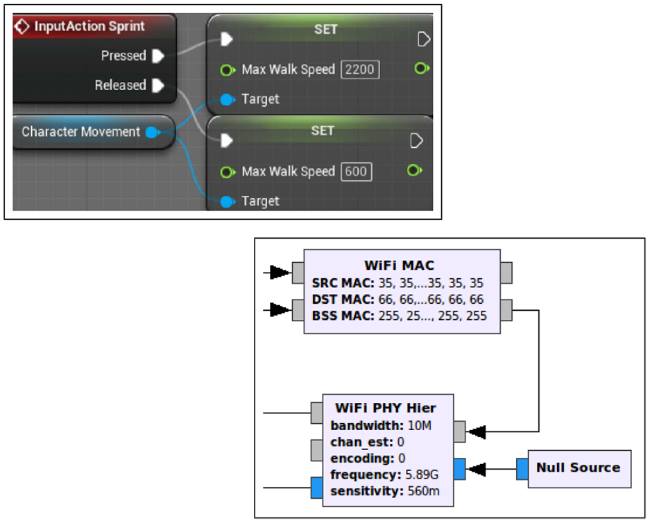
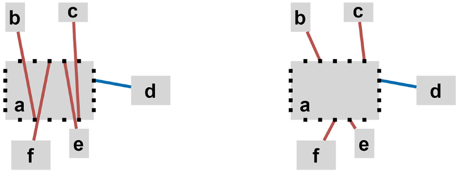
Complex relational structures in graphs are often better modeled by introducing constraints on the locations where links are connected to their incident objects. These dedicated connection points, called ports, heavily influence how the models should be visualized (Figure 1).
There has been plenty of work done on general graph layout 2 but considerably less on compound graphs. 7 Most such work ignores node dimensions (or assume them to be uniform) and neglects specific connection points of edges to nodes, both of which are common requirements in real-life maps (Figure 1). Toward this end, we present a new layout algorithm CoSEP, which builds on a previous compound spring embedder algorithm named CoSE, 7 and adds support for port constraints on edges while respecting non-uniform node dimensions and compound structures in straight-line drawings such as languages used to represent biological, financial transaction, and visual scripting networks.5,8,9
Background
A graph or a network is a representation of a discrete set of objects, called nodes, where object pairs are joined by links, called edges. An edge is said to be incident on its source and target nodes. For an undirected bidirectional edge
Source and target nodes of an edge are said to be adjacent. A path in a graph is a sequence of edges with common end nodes, connecting a sequence of non-repeating nodes. A graph is disconnected if at least two nodes of the graph are not connected by a path. A tree is a graph where all node pairs are connected by exactly one path. A rooted tree is a tree with a fixed number of nodes, in which a particular node is distinguished from the others, called the root.
A compound or hierarchical graph
A compound graph
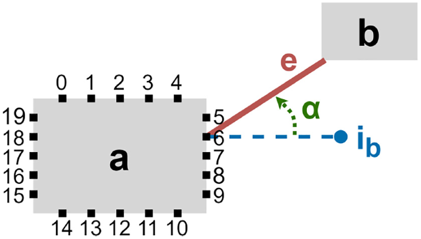
Within the scope of this work, we assume nodes to have a rectangular geometry with ports (i.e. connection points) distributed along the edge of the associated rectangle, an equal number on each side (Figure 3). In cases where nodes can have varying number of ports on each side or ports can have arbitrary user-specified positions, a cyclic ordering of all ports of a node could be calculated beforehand and maintained in a data structure which allows constant time access to both the predecessor and successor of a particular port in this ordering. This way edge endpoints could be shifted as required by an algorithm without an impact on the asymptotic runtime efficiency of the algorithm.
An edge
We further assume that any node, including compound nodes and those nested inside compound ones, is allowed to have port constraints defined on its incident edges. An edge may have a possibly different port constraint on each end, chosen from the following types:
A drawing or layout of a graph is a function mapping each node to a distinct point and each edge to a Jordan curve, with endpoints corresponding to end node locations. 2 Automatic layout aims to create a drawing of the input graph that is as clear and pleasant as possible. A poor layout is likely to confuse the user, while a well-organized and aesthetically pleasing one usually improves the users understanding of the underlying relational data. While good layout criteria are subjective, the generally accepted ones 2 include minimal total drawing area, number of edge–edge crossings and total edge length, yielding uniform edge lengths, and reflecting any symmetries in the graph. Most layout algorithms start with nodes at random positions or produce positions from scratch. But, in cases where the user would like the layout algorithm to respect the current positions while tidying up the drawing with respect to commonly accepted graph drawing criteria, an incremental layout is preferred.
Force-directed layout algorithms (aka spring embedders) are a popular approach to automatic graph layout. 2 The basic idea is to simulate a physical system obeying the laws of Newton, Hooke, and Coulomb, in which nodes behave as electrically charged physical entities, and edges are represented by physical springs of a specified ideal length. Springs exert forces to their connected objects proportional to the deviation from their “natural” length. In order to avoid node-to-node overlaps and to evenly space nodes out (by a user-specified ideal edge length away from each other), entities that are too close repel each other. The layout algorithm simulates this underlying physical model by moving entities corresponding to nodes iteratively with respect to total forces acting upon them, until the system of entities reaches a relatively stable state, in which the overall energy is minimal. Force-directed layout algorithms typically use a cooling schedule via a cooling factor to enforce a convergence. 2
In addition to these main forces, there are relatively minor gravitational forces that keep graph components (when the graph is disconnected) together.
The following are the additions made to this basic model by the CoSE algorithm to support compound graphs 7 :
Compound nodes are handled by representing an expanded node and its associated nested graph as a single entity, similar to a “cart,” which can move freely.
The length of an edge is defined to be the length of the line segment going through one end node’s center to the other, clipped on both sides by the rectangles representing the end nodes. In the case of port constrained edges, we modify this definition as follows. If a particular edge end is port constrained, then the length is calculated starting from the port location without a need for clipping and ignoring any edge-node intersections.
Compound nodes consisting of only disconnected nodes are tiled to create a compact and elegant layout. 11
Layered graph drawing or hierarchical layout is a layout style where the nodes of a directed graph are drawn in horizontal rows (vertical columns) or layers with the edges generally directed downwards (toward the right) 2 to emphasize flows (e.g. data flow diagrams). This approach is mainly composed of layer assignment, crossing reduction, and final x-coordinate (y-coordinate) assignment steps. The most common method in reducing crossings in between two consecutive layers is using the so-called barycenter method. This heuristic is simply based on placing a node at the barycenter (average) of the x-coordinates (y-coordinates) of its neighbors. This style is used by many algorithms addressing port constraints as discussed in related work.
Certain domains explicitly make use of a so-called orthogonal edge style, including those using a hierarchical layout, where edges are routed with horizontal and vertical edge segments only. 2
Related work
Many graph drawing algorithms have been proposed to visualize port constrained graph models such as data structure maps, data flow diagrams, schematics of digital circuits, and biochemical networks. The work done on data structures12–14 utilizes ports as pointers connecting various complex structures to each other. Due to the nature of data structures, these works do not support multiple types of port constraints. An added port constraint can only restrict an edge endpoint to a fixed position around a node. With techniques such as spline curve edge routing, rotating nodes, barycenter heuristic, and dummy nodes, these fixed edge endpoints are integrated into the layer-based approach, especially suitable for directed graphs.
The work in Battista et al. 15 describes a way to draw database schemas in which database tables are depicted as rectangular boxes consisting of table attributes. Edges, called links, connect two different table attributes together representing referential constraints or join relationships. These edges can connect to their respective attributes only from the right or left side of the associated table row (Figure 4), which is a good example of a rather special type of domain-specific port constraint.
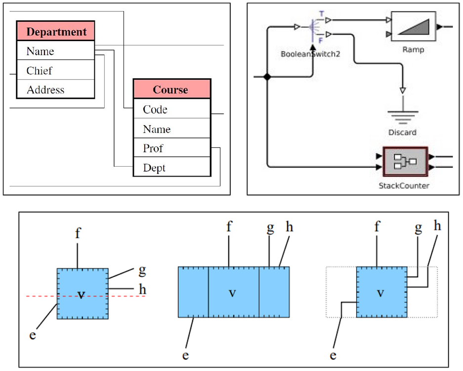
Part of a database schema making use of ports for attribute relationships (top-left), part of a data flow diagram representing a stack (top-right), an example of Siebenhaller’s technique of rerouting right and left side ports to top or bottom (bottom).
The series of published work by Schulze et al. 16 and a follow-up work by Schelten 17 improving inter-graph edge crossings across multiple nesting levels via a post-processing step are for visualizing data flow diagrams, also using the layer-based approach. They develop several extensions to the barycenter heuristic to support port constraints. They have defined five different levels of port constraints to cover the requirements of data flow diagrams (Figure 4). The level of a port constraint ranges from “flexible” to “restrictive.” Therefore, the main algorithm, which has five phases, transitions port constraints down this hierarchy in each phase. In the end, each port constraint is reduced to a definitive position relative to its node. Similarly, the solution is focused on the nature of data flow diagrams, where nodes are hierarchical and the main orientation of edges are left to right (or top to bottom). Walter et al. 18 also apply a very similar approach, modifying each phase for the layered drawing of undirected graphs with a special focus on drawing cable plans of complex machines. The study by Regg et al. 19 addresses the same problem but using a constrained-based approach. Due to the excessive use of constraints, however, their algorithm deeply suffers from poor execution time. Unfortunately, both approaches work only for a more restricted type of compound graphs where edges are not allowed to directly connect to compound nodes.
Earlier work by Genc and Dogrusoz 20 uses the force-directed layout scheme to address the conventions of Process Description (PD) maps of the Systems Biology Graphical Notation (SBGN) by employing additional heuristics. These heuristics mainly strive to satisfy sided port constraint rules and try to place substrate (input) and product (output) biological entities on opposite sides of process nodes.
Siebenhaller 21 defines port constraints in orthogonal graph drawings with more flexibility. Similar to our approach, ports are distributed evenly around the node, constraints are associated with edges, and not every edge has to be port constrained. As depicted in Figure 4, they reroute a node’s right and left side ports locally to the top or bottom with an edge bend. In order to reduce edge crossings, they further transform the problem to a minimum cost flow network. The algorithm is shown to work on UML activity diagrams.
All of the previous work mentioned here focus on simple graphs or on restricted compound graphs drawn with orthogonal edges. Our work, on the other hand, aims to create flexible straight-line drawings, which happens to be the desired style of drawing in many real-life applications and can handle compound graphs. Furthermore, with the help of our coverage for varying port constraints, our algorithm is applicable to a wider range of domains such as biological and visual scripting languages.
Methods
The proposed automatic layout algorithm is based on integrating port constraints into the CoSE layout algorithm. 7 Additional heuristics and related forces are added on top of the existing force-directed model of CoSE. The following is a brief summary of the additions to be detailed later on, in related sub-sections:
Port constrained edge endpoints are allowed to shift to adjacent ports that they are connected to, in order to remove the rigidness due to discrete port positions.
In some cases, shifting edge endpoints is not enough on its own to remove the edge crossings around a node with ports. In such cases, the layout may be improved by rotating the node by
Additionally, relatively smaller forces are applied to move nodes incident to port constrained edges to their ideal positions (right across the port, an ideal edge length distance – defined by the user – away from the port) defined by the port location.
The algorithm tries to move a degree-one node that is incident to an edge whose other end is port constrained to its ideal location. In some cases, having multiple such nodes can cause a local deadlock. Hence, a supplementary heuristic is added to periodically carry these nodes to their ideal positions.
Underlying physical model
Our underlying algorithm is a basic force-directed layout further extending the force model of the CoSE algorithm with some heuristics to satisfy the port constraints.
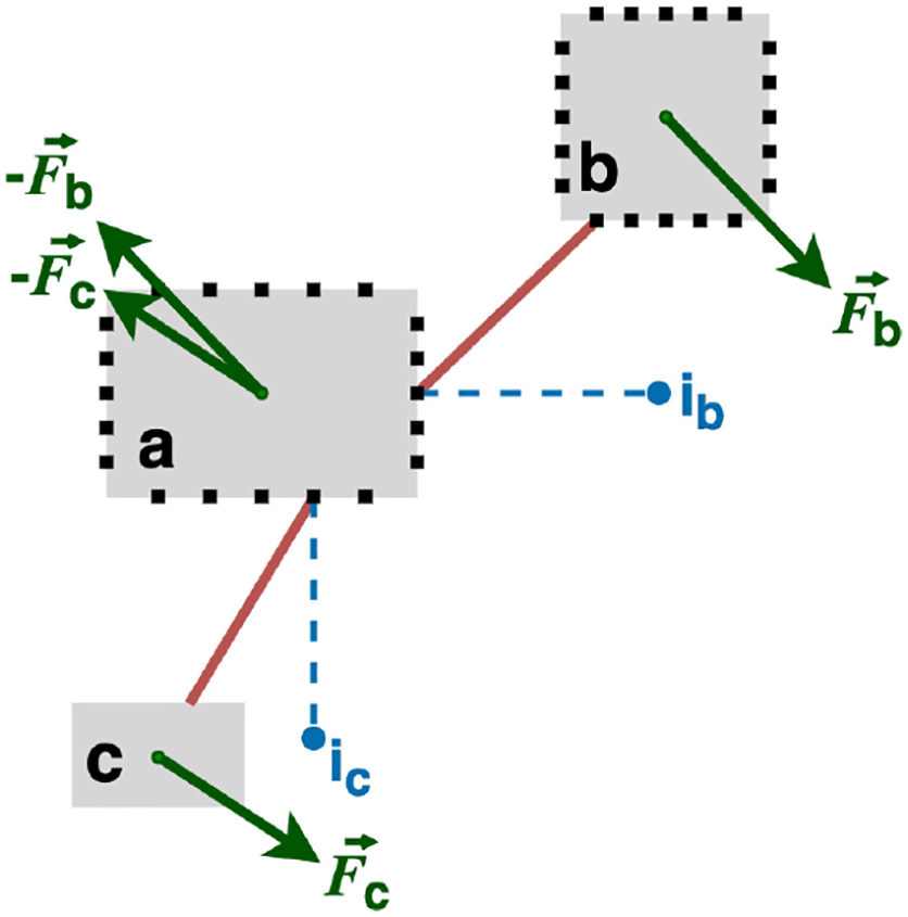
To do so, we explicitly make use of rotational forces. The rotational component of a spring force due to an edge
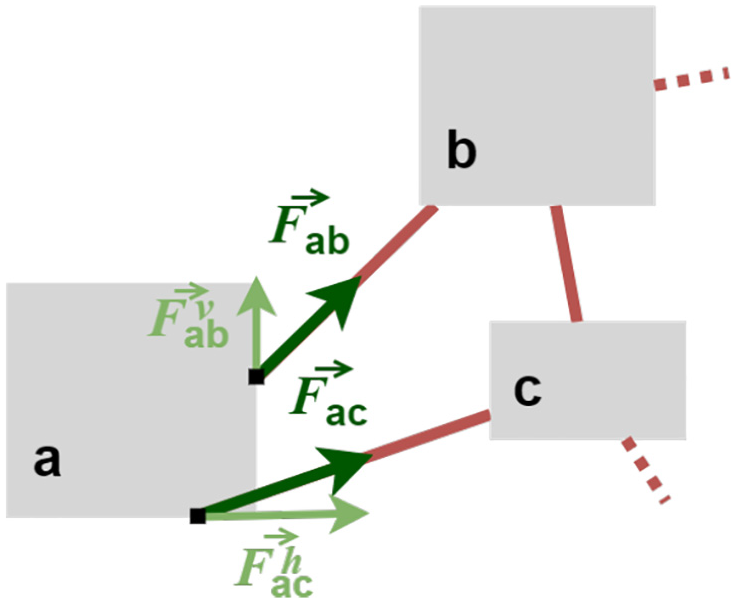
Spring forces
Shifting edge endpoints
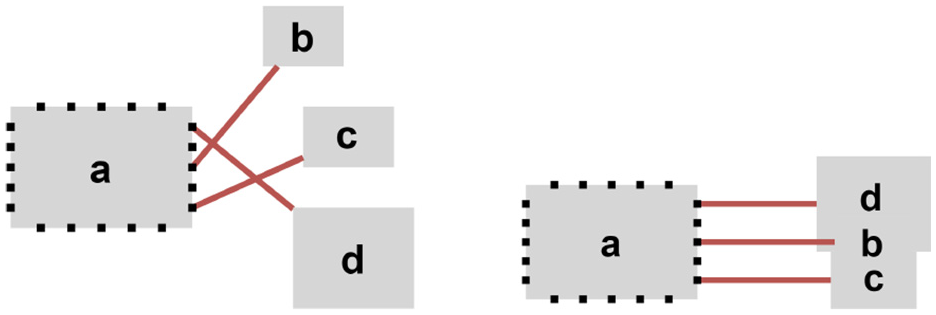
Quite often, an edge endpoint that has a port constraint would like to move to an adjacent port to be closer to the incident node on its other end. We allow such edge ends to shift to ports toward a better/closer location unless the port constraint prevents that. Allowing such shifts typically reduce edge crossings around a node introduced by port constraints (Figure 6).
A node
Generally in force-directed layouts, spring forces are utilized solely to move nodes around. We make use of the rotational component of these spring forces to shift edge endpoints (and to rotate nodes when necessary as discussed later on) as well. For each edge endpoint, associated rotational forces induced on the port are averaged over a number of pre-defined iterations. If this average is bigger than an edge shifting threshold, the edge is shifted clockwise or counterclockwise. Rather than applying this heuristic at each iteration, we average over a number of pre-defined iterations to avoid potential oscillations, making sure the shift is for the better.
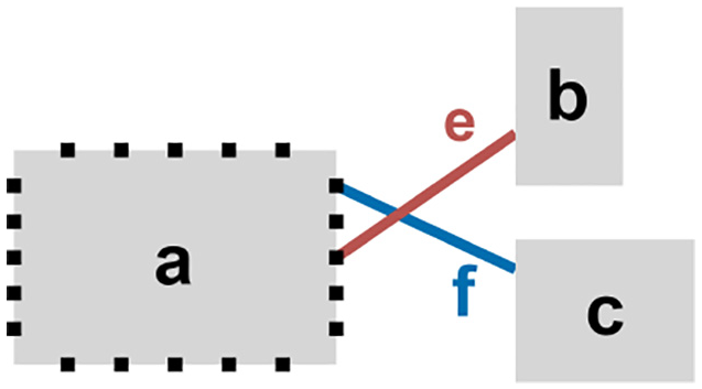
While shifting an edge endpoint, we also permit the endpoint to change sides, assuming the associated port constraint allows this new port location. For instance, assume that in Figure 3, the edge endpoint located at port index 6 was instead connected to the port at index 10. In that case, it would be viable to shift the edge endpoint to port at index 9 since node
In order to avoid oscillations due to shifting to a port at another side, we not only pay attention to the total rotational forces over a number of iterations but also to the current orientation of the end nodes. In situations where shifting to the adjacent, the nearer side is allowed, the other end node (or the port if that edge end also has a port constraint) has to be in a certain relative position in order to proceed with the shift operation. This respective location is based on a diagonal line that goes through the center of the node and the corner of the node residing between associated sides (Figure 7).
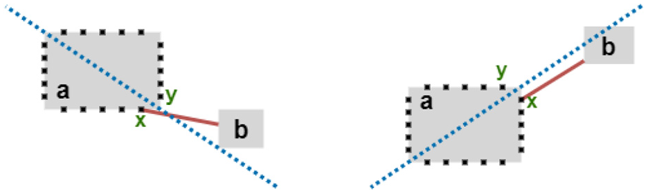
The dashed line indicates the other edge end’s position requirement for edge end shifting between neighboring node sides. The edge end at port
In the case where the adjacent side is not available (e.g. source of
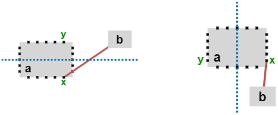
Similar to Figure 7, the dashed line marks the border for the position requirement for edge end shifting between opposite node sides. The edge end at port
Rotating nodes or swapping opposite sides
For certain port configurations, the overall topology of the graph and the current positioning of the graph objects can be too restrictive on some edges. In such situations, shifting edge endpoints alone might be ineffective in avoiding edge crossings. Thus, we sometimes resort to a more drastic change on nodes and either rotate them by
The rotational forces come in handy for this heuristic as well. The idea behind the heuristic is that if incident edges of a node are repeatedly and consistently pushing or pulling the node toward a certain direction, rotating the node accordingly can turn the overall system into a more stable state, quicker than slowly shifting individual edge endpoints. In certain cases, port constraints might not allow such shifts anyway.
If the averaged net rotational force
An example, where the 90° rotation heuristic fails to detect an unstable circumstance (left). The same graph where a swap of ports on opposite sides (top and bottom here) was performed on node
There are two types of swaps:
Instead of the rotational force scheme, the swap heuristic utilizes the angle that a port constrained edge makes with the ray starting from the associated port and going toward the node’s ideal position (Figure 3). So as to determine whether or not a swap would be beneficial, the algorithm checks if the majority of neighboring nodes have obtuse angles. For instance, neighboring nodes for the
In order to avoid drastic changes and keep the layout more stable, a node can either rotate by 90° or its ports on opposite sides are swapped in one iteration but not both. There is no limit on how many rotations or swaps a node can make over the course of all iterations though.
Moving nodes to their ideal positions
In some graph models, local positioning of nodes connected together with port constrained edges has an implicit meaning (a note node associated with a specific method of a class in a UML class diagram), mapping the port to the matching degree-one node. In order to fulfill this convention and provide an aesthetically pleasing layout, we introduce an additional force type into the force scheme named polishing force that pushes such degree-one nodes to their ideal positions. However, we do not want to interfere with the overall force-directed system here. Thus, the magnitude of this type of force is relatively weaker than spring or repulsion forces. Similar to the gravitational force, its magnitude is calculated to be the distance (to the ideal position) times some constant decided empirically. The direction of the force is orthogonal to the edge and toward the ideal location, which is estimated to be an ideal edge length away across the port location (Figure 10).
A node
Notice however that this new force is not only applied to the degree-one node to move it to its ideal position but also to the other end node with the associated port. Thus, the overall force-directed system is preserved under Newton’s third law (i.e. every action requires an opposite reaction with equal magnitude).
Further handling of degree-one nodes
Generally, polishing forces defined above are sufficient on their own to reduce edge crossings. However, when port constraints are too restrictive or when a node is incident to too many port constrained edges, polishing forces fail in reducing edge crossings. In cases such as the one in Figure 11, polishing forces will not be able to overcome the spring and repulsion forces resulting in a stalemate. Thus, a special procedure is put in place to periodically move degree-one nodes incident to a port constrained edge to their ideal positions. This heuristic is executed multiple times because such drastic node movement can cause node overlaps making the local state unstable. By insisting on this placement, we make sure the neighboring nodes spread out, not undoing the improvement by this heuristic.
A node
Algorithm
In order to properly integrate port constraint support, the new algorithm extends the CoSE algorithm to five phases, including the initialization phase. Three of these phases (phases II, III, and IV) contain the newly introduced heuristic procedures. Hence, the major steps of CoSEP are as follows (refer to Figure 12 for a working example):
Initialization: In this part, the necessary drawing model for the CoSE algorithm is constructed. Nodes are scattered randomly across the drawing space unless the layout is to be performed incrementally, and the convergence threshold is set according to the number of nodes.
Phase I: In order to establish a “skeleton” layout, the CoSE algorithm with a minimal, reduced number of iterations is performed on the whole graph. Since only a rough starting configuration is needed (to be later polished by succeeding phases), using CoSE’s “draft” layout quality should be sufficient.
Phase II (initializing ports): Port constrained edge endpoints are assigned to feasible “corner ports” that are closest to the other end node’s center. For instance in Figure 3, assume that there is a fixed side
Phase III: The spring embedder starts again with a lower cooling factor. Rotational forces and angles of edge endpoints, necessary for various heuristics, are calculated together with spring, repulsion, and gravity forces. The heuristic procedures of shifting endpoints, rotating nodes, and handling degree-one nodes are performed in this phase.
Phase IV (polishing phase): In contrast to Phase III, only the heuristics related to the handling of degree one nodes are applied. Furthermore, the initial cooling factor is even lower than Phase III as this phase is expected to minimally alter the established layout.
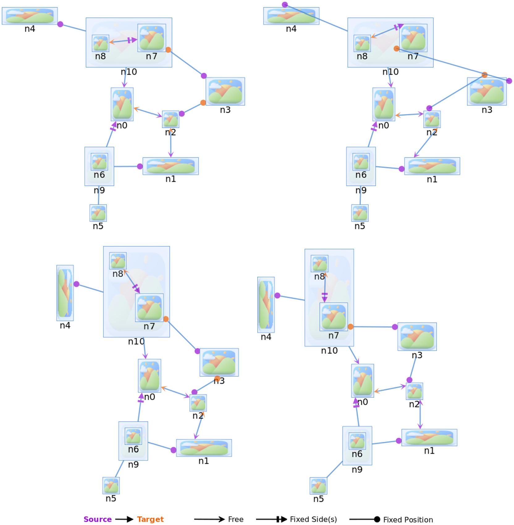
A sample compound graph with various port constraints after Phase I (top-left), Phase II (top-right), Phase III (bottom-left), and Phase IV (bottom-right). Various heuristics can be seen in action during this layout as follows. During Phase III, node
The major steps mentioned above can be integrated into the CoSE algorithm by expanding its main method as in Algorithm 1.
The CoSEP algorithm.
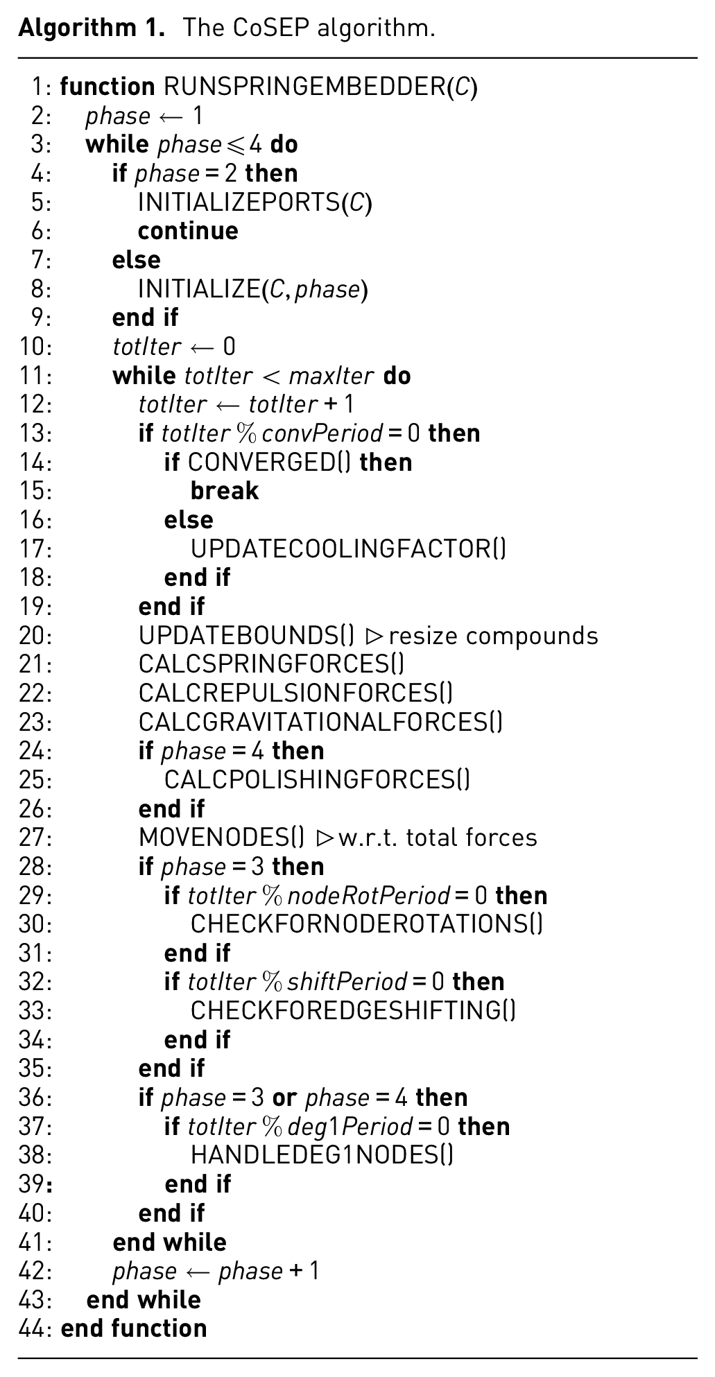
Notice here that not all heuristics are applied at each phase. For similar efficiency reasons, within a phase, these heuristics are applied sparingly (i.e. not at each iteration of the phase). This is true for convergence checks as well. How often each is to be applied or checked for was determined empirically.
Phase II is solely composed of initialization of ports. Hence, we continue after this initialization, skipping force calculations, etc. In all other phases though, we initialize parameters such as the initial cooling factor with respect to the particular phase’s requirements as explained earlier. Further notice that as nodes are relocated, compound node bounds need to be updated accordingly.
Time complexity
The running time of the CoSE algorithm is
Evaluation
For evaluating our new algorithm, we used the following performance criteria: number of edge crossings, number of node to node overlaps, average edge length, total area, ratio of properly oriented port constrained edge ends to the overall number of port constrained edge ends, and execution time. Here, all criteria except the last one measure the quality of the resulting layout, whereas the last one measures the execution speed. Among these, all are commonly used graph layout success criteria,
2
except properly oriented edge ends that we specifically introduce for port constrained layout. An edge end is deemed as “properly oriented” if the edge’s line segment does not intersect with the rectangle of the associated end node. For instance, for the left graph in Figure 9, all of the four edge ends on top and bottom side of node
We decided to compare our algorithm with CoSE as no other previous related work will properly handle compound structures in graphs or use straight-line representations for edges. Note that the algorithm of Schulze et al. can layout data flow diagrams with compound nodes in a bottom-up manner. However, in their approach, the algorithm is applied to each graph separately, without paying attention to inter-graph edges, which is the inherently hard part of compound graph layout. In addition, the type of constraints supported by previous other work is not fully compatible with those of CoSEP. Furthermore, the main aim of this work has been to add constraint support to a layout algorithm for compound graphs with non-uniform node dimensions.
Figures 13 and 14 show some sample layouts produced by our algorithm in comparison with CoSE. Please refer to the demo at https://ivis-at-bilkent.github.io/cytoscape.js-cosep/demo/demo.html on GitHub for more examples.
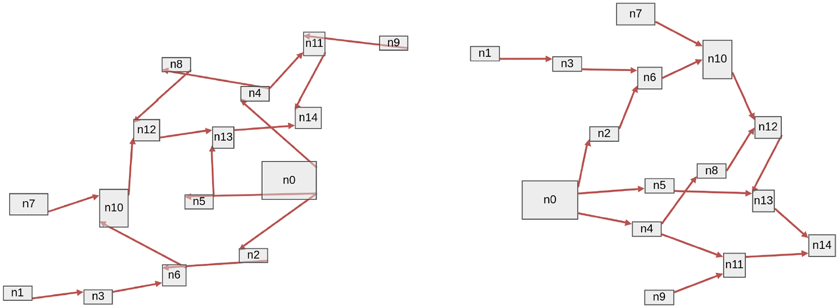
A visual scripting graph 5 is laid out with CoSE (left) and CoSEP (right) using Fixed Side(s) constraints. Respective metrics (CoSE–CoSEP): ratio of properly oriented edge ends: 35.29%–91.17%, number of edge-edge crossings: 4–1, running time: 9.65–23.81 ms.
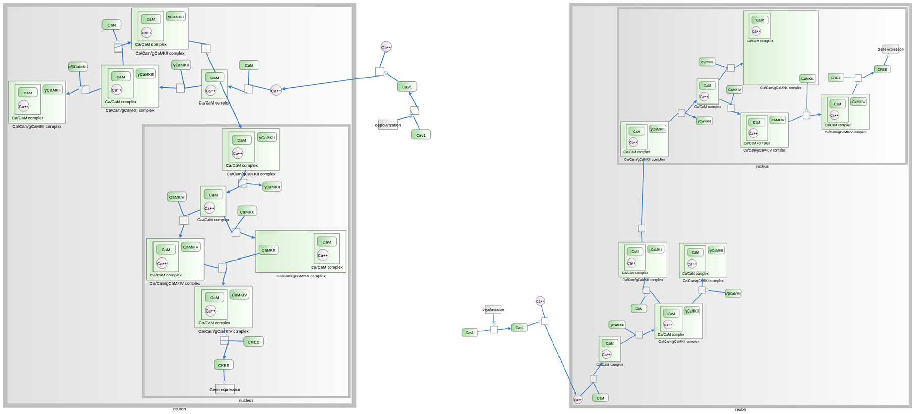
An SBGN PD map illustrating CaM-CaMK dependent signaling to nucleus is laid out with CoSE (left) and CoSEP (right) using Fixed Side(s) and Fixed Position constraints. Respective metrics (CoSE–CoSEP): ratio of properly oriented edge ends: 46.14%–97.14%, number of edge-edge crossings: 3–0, running time: 31.83–73.36 ms.
Setup
We implemented and tested the CoSEP algorithm in JavaScript as an extension to Cytoscape.js, 24 an open-source library for graph analysis and visualization. The experimentation was done on a PC running Linux with an Intel Core i7-4790 3.6 GHz processor and 16 GB of RAM.
We tested our algorithm CoSEP in comparison to the CoSE algorithm with a test suite, the set named RND/BU4P in reference
25
of randomly generated biconnected, undirected, and 4-planar graphs, which has been widely used in graph drawing studies.26,27 Among the
We conducted experiments to see the behavior of our algorithm as graph size changes. We also wanted to observe how the performance changes as the type and amount of port constraints change.
In order for a fair comparison of CoSE with ours in terms of satisfying port constraints, we decided to assign ports to edge ends in a systematic way as opposed to a random one. Hence, we used Phase II (initializing ports) of CoSEP for figuring out an implied port location for each edge end after CoSE completes. Results of all these experiments can be found in Figures 15 to 27 and are discussed below.
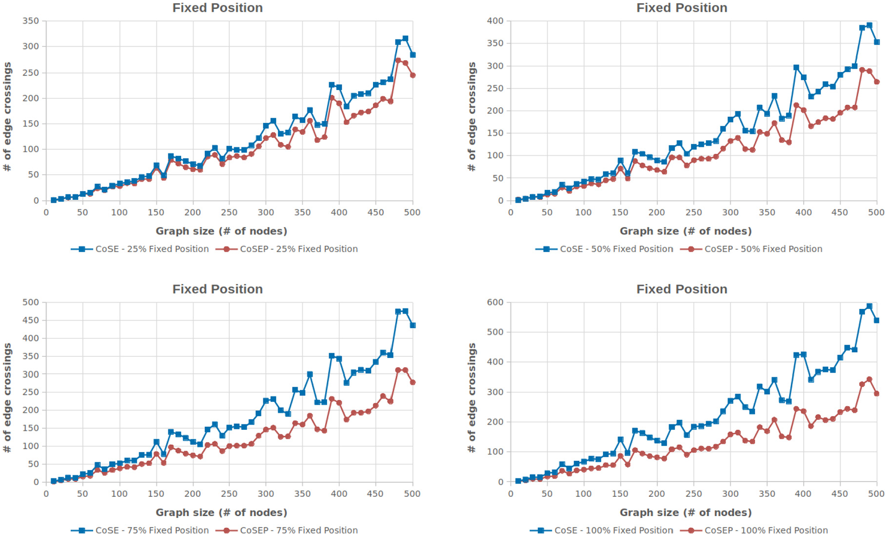
Number of edge crossings versus number of nodes of our algorithm (CoSEP) in comparison with CoSE. In (top-left) 25%, (top-right) 50%, (bottom-left) 75%, (bottom-right) 100% of the edge ends are port constrained. The percent value here denotes the ratio of edge ends with port constraint Fixed Position to the total number of edge ends.
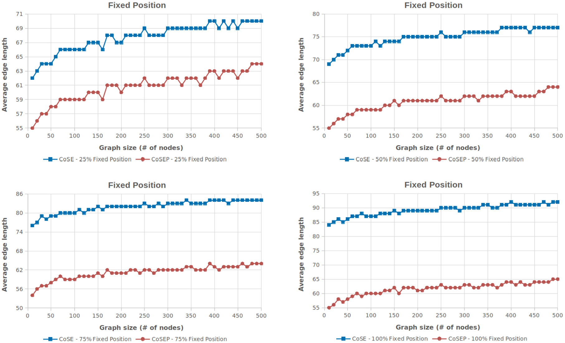
Average edge length versus number of nodes of our algorithm (CoSEP) in comparison with CoSE. In (top-left) 25%, (top-right) 50%, (bottom-left) 75%, (bottom-right) 100% of the edge ends are port constrained. The percent value here denotes the ratio of edge ends with port constraint Fixed Position to the total number of edge ends.
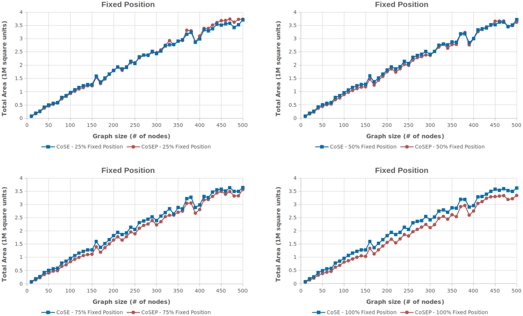
Total area (in 106 square units) versus number of nodes of our algorithm (CoSEP) in comparison with CoSE. In (top-left) 25%, (top-right) 50%, (bottom-left) 75%, (bottom-right) 100% of the edge ends are port constrained. The percent value here denotes the ratio of edge ends with port constraint Fixed Position to the total number of edge ends.
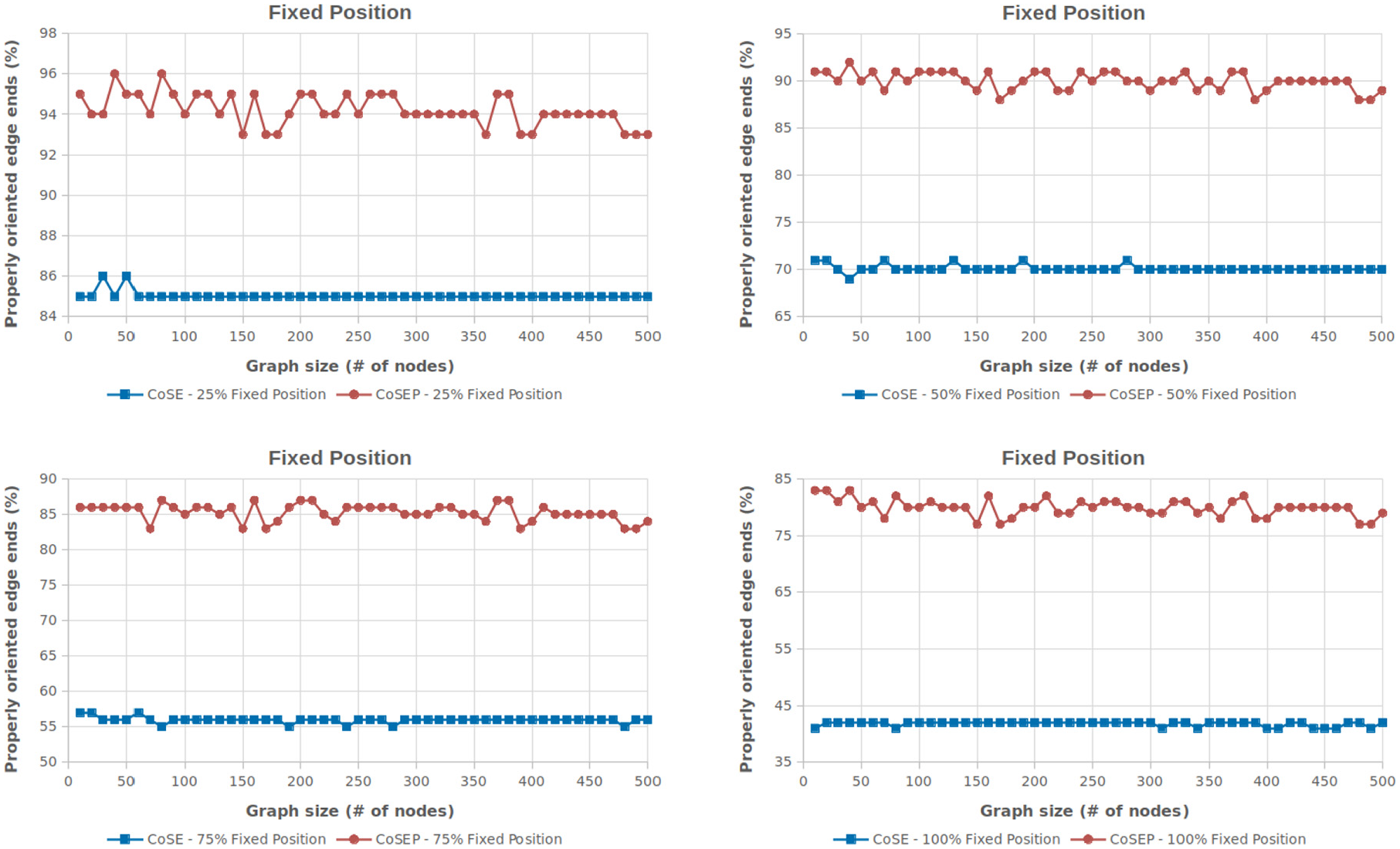
Ratio of properly oriented edge ends versus number of nodes of CoSEP and CoSE. In (top-left) 25%, (top-right) 50%, (bottom-left) 75%, (bottom-right) 100% of the edge ends have Fixed Position port constraint. The percent value here denotes the ratio of edge ends with port constraint Fixed Position to the total number of edge ends.
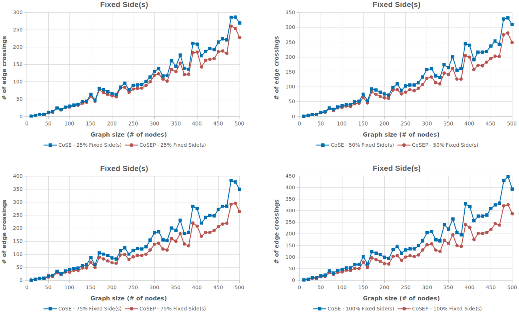
Number of edge crossings versus number of nodes of our algorithm (CoSEP) in comparison with CoSE. In (top-left) 25%, (top-right) 50%, (bottom-left) 75%, (bottom-right) 100% of the edge ends are port constrained. The percent value here denotes the ratio of edge ends with port constraint Fixed Side(s) to the total number of edge ends.
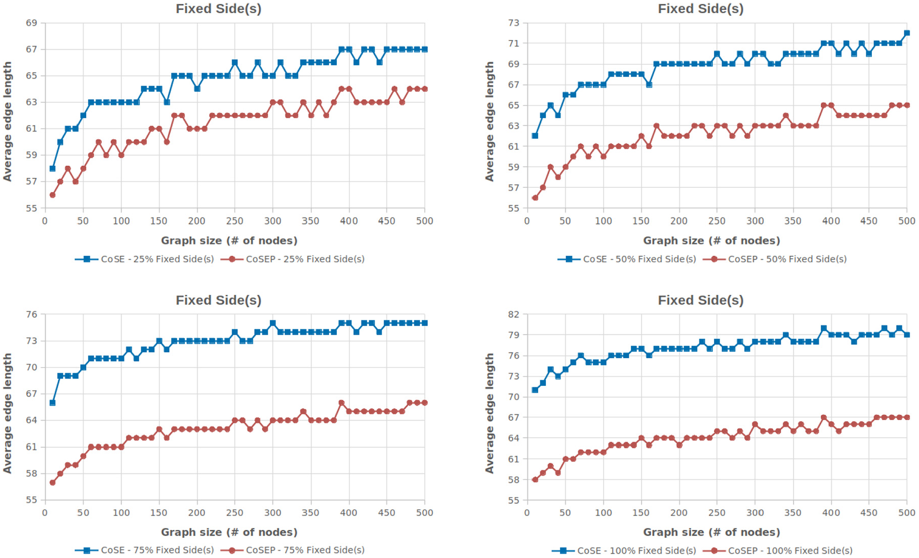
Average edge length versus number of nodes of our algorithm (CoSEP) in comparison with CoSE. In (top-left) 25%, (top-right) 50%, (bottom-left) 75%, (bottom-right) 100% of the edge ends are port constrained. The percent value here denotes the ratio of edge ends with port constraint Fixed Side(s) to the total number of edge ends.
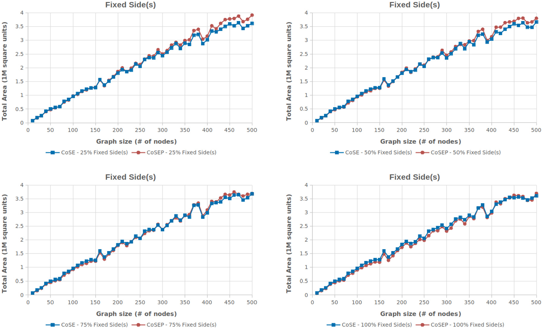
Total area (in 106 square units) versus number of nodes of our algorithm (CoSEP) in comparison with CoSE. In (top-left) 25%, (top-right) 50%, (bottom-left) 75%, (bottom-right) 100% of the edge ends are port constrained. The percent value here denotes the ratio of edge ends with port constraint Fixed Side(s) to the total number of edge ends.
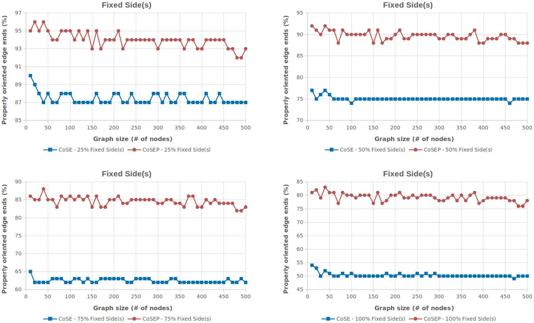
Ratio of properly oriented edge ends versus number of nodes of CoSEP and CoSE. In (top-left) 25%, (top-right) 50%, (bottom-left) 75%, (bottom-right) 100% of the edge ends have Fixed Side(s) port constraint. The percent value here denotes the ratio of edge ends with port constraint Fixed Side(s) to the total number of edge ends.
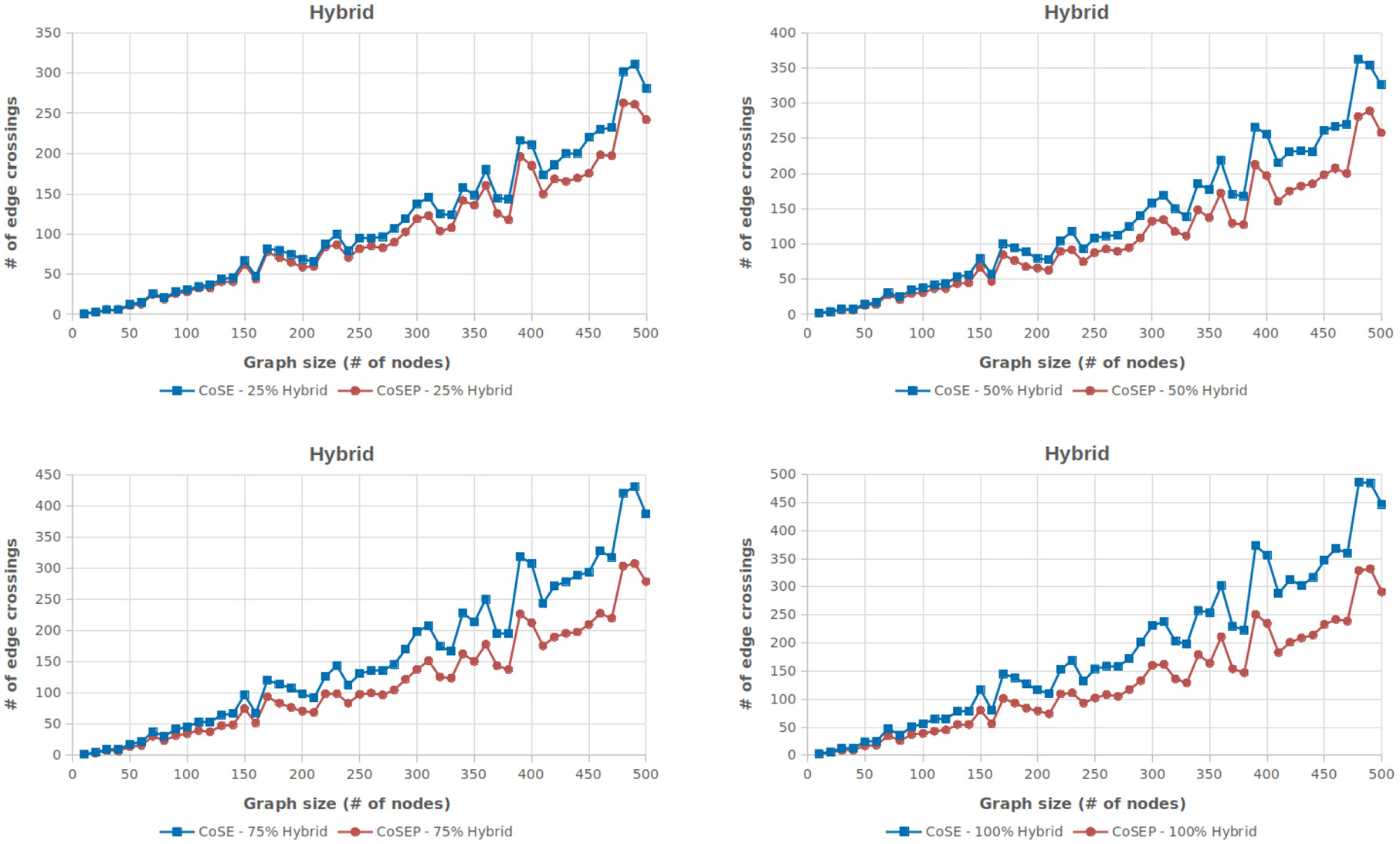
Number of edge crossings versus number of nodes of our algorithm (CoSEP) in comparison with CoSE. In (top-left) 25%, (top-right) 50%, (bottom-left) 75%, (bottom-right) 100% of the edge ends are port constrained. The percent value here denotes the ratio of edge ends with port constraint either Fixed Position or Fixed Side(s) to the total number of edge ends.
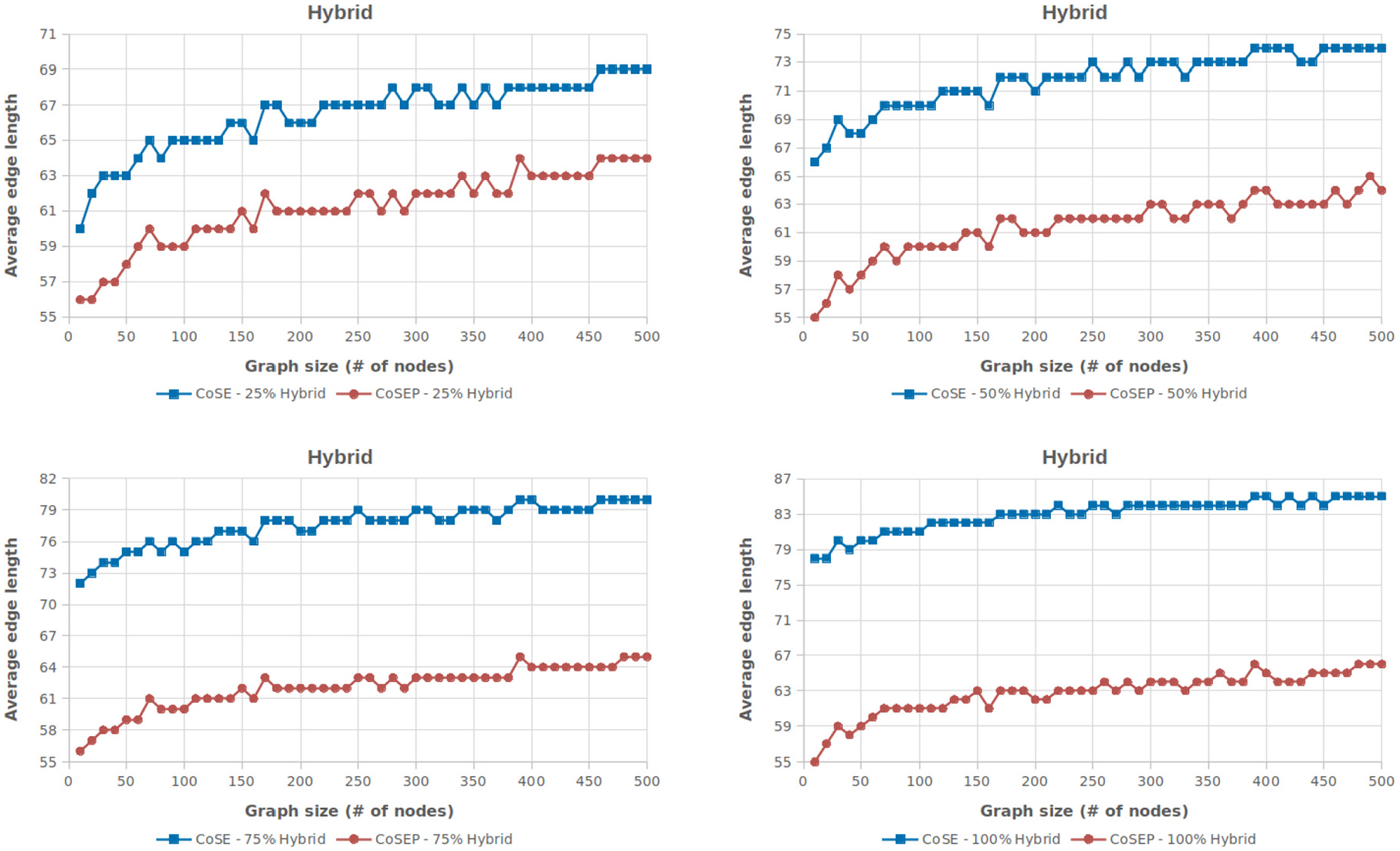
Average edge length versus number of nodes of our algorithm (CoSEP) in comparison with CoSE. In (top-left) 25%, (top-right) 50%, (bottom-left) 75%, (bottom-right) 100% of the edge ends are port constrained. The percent value here denotes the ratio of edge ends with port constraint either Fixed Position or Fixed Side(s) to the total number of edge ends.
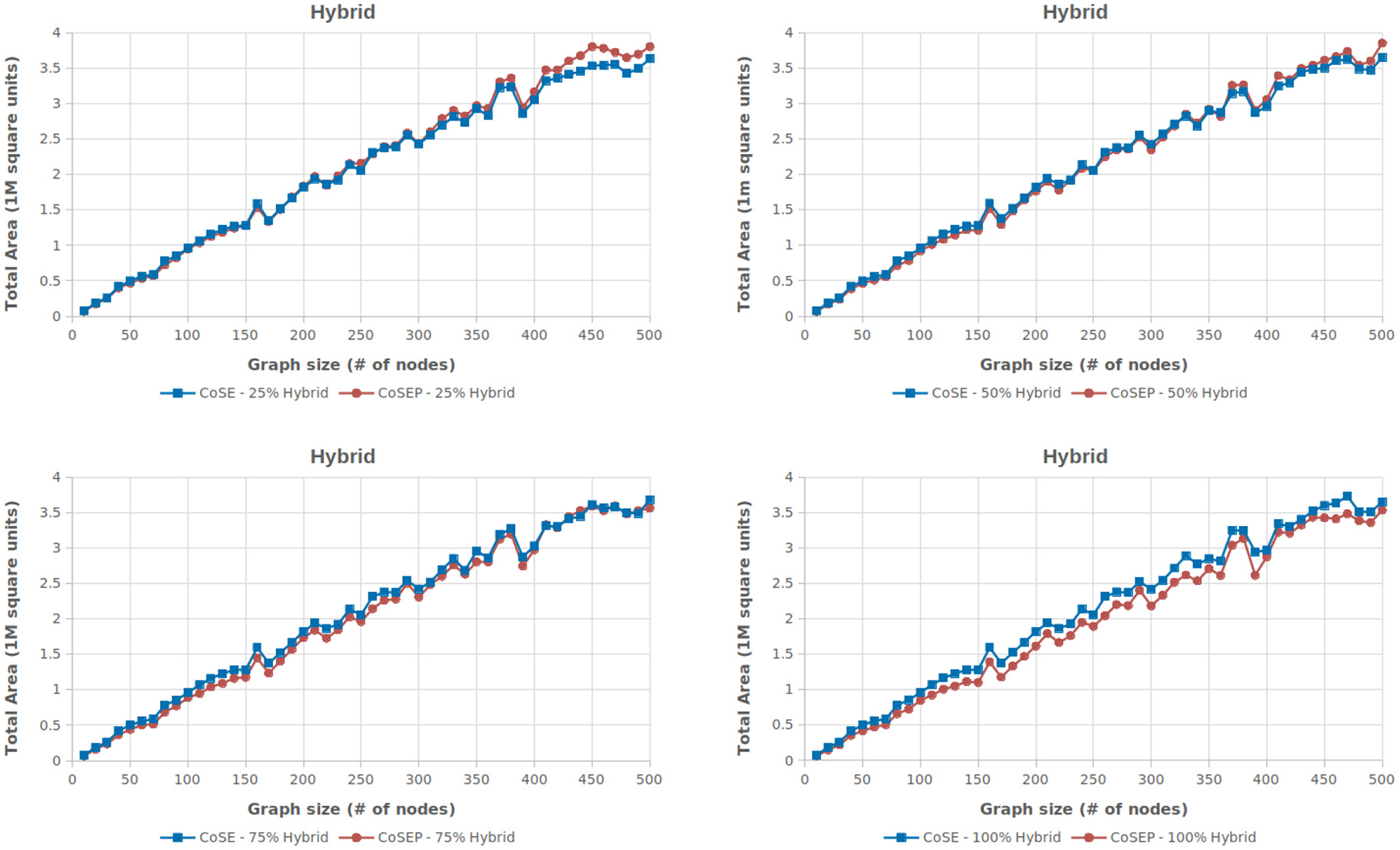
Total area (in 106 square units) versus number of nodes of our algorithm (CoSEP) in comparison with CoSE. In (top-left) 25%, (top-right) 50%, (bottom-left) 75%, (bottom-right) 100% of the edge ends are port constrained. The percent value here denotes the ratio of edge ends with port constraint either Fixed Position or Fixed Side(s) to the total number of edge ends.
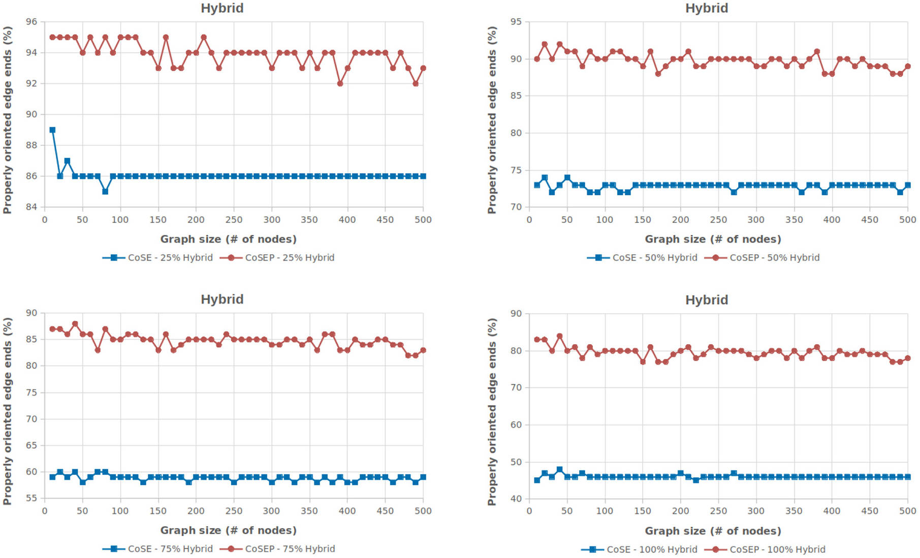
Ratio of properly oriented edge ends versus number of nodes of CoSEP and CoSE. In (top-left) 25%, (top-right) 50%, (bottom-left) 75%, (bottom-right) 100% of the edge ends are port constrained. The percent value here denotes the ratio of edge ends with port constraint either Fixed Position or Fixed Side(s) to the total number of edge ends.
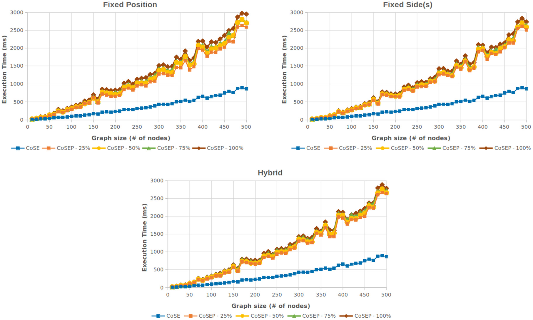
Comparison of the running time of our algorithm with varying proportions of the edges with port constraints (CoSEP) with CoSE (graph size versus execution time in milliseconds). Edge ends can only have Fixed Position constraint in (top-left), Fixed Side(s) constraint in (top-right), and can have both port constraints in (bottom). The percent value here denotes the ratio of edge ends with port constraint to the total number of edge ends.
Experimental results
Quality
In general, our algorithm produces comparable results to CoSE with respect to above-mentioned criteria. In our experiments, there is almost no node-to-node overlap in any graph for both CoSE and CoSEP algorithm. This is due to the fact that repulsion forces are successfully separating nodes.
Since CoSE does not have support for port constraints, it naturally fails to yield drawings that are satisfactory in terms of general graph drawing criteria such as number of edge crossings (Figures 15, 19, and 23) and average edge length (Figures 16, 20, and 24). When the edge ends are scarcely port constrained, CoSE does a decent job in delivering a good layout. Yet, as edge ends get increasingly port constrained, CoSEP noticeably dominates CoSE. For instance, when only Fixed Position port constraint is added to edge ends, our novel heuristics in CoSEP reduces the number of edge crossings significantly (Figure 15). This edge crossing reduction is 13%, 21%, 34%, and 41%, respectively in the order of increasing Fixed Position port constraints. The experiments in Figures 19 and 23 show a similar result. Evidently, the performance gap between CoSE and CoSEP is immense in experiments in Figures 15 and 16 as opposed to those in Figures 19, 20, 23, and 24 since Fixed Position constraints are harder to handle. A similar behavior, although not as drastic, is observed for total area (Figures 17, 21, and 25).
Experiments for ratio of properly oriented edge ends paint a similar picture. As Figures 18, 22, and 26 demonstrate, the success of CoSE is not far behind CoSEP when the edge ends are moderately constrained. But, the success of CoSE dips substantially afterward. When all the edge ends are port constrained, CoSE provides a layout where there are too many node-edge intersections. In such cases, CoSE clearly fails to produce an “aesthetically pleasing” result.
Running time performance
From the theoretical analysis given earlier, a quadratic behavior of execution time is expected of CoSEP. The experiments validate this argument (Figure 27). Even though CoSEP has the same asymptotic running time complexity as CoSE, the additional heuristics and new phases to CoSE increase the iteration count of the overall spring embedder. This clearly slows down the CoSEP in practice. However, the overall run time is acceptable for interactive visual analysis components, assuming the component deals with graphs up to several hundred nodes, and for larger graphs, complexity management techniques 4 are employed to reduce the graph size.
Conclusion
This paper describes a new algorithm CoSEP for automatic layout of general compound graphs with support for constrained connection of edges to their source/target nodes. When tested with graphs with a size suitable for interactive visualization, CoSEP performs rather well both in terms of the quality of the resulting layout and its speed.
Potential future work includes fine-tuning of various phases and the use of GPU processing to improve run-time performance. In addition, we could measure how long it takes to execute iterations and then decide dynamically when to apply the additional heuristics, rather than using empirical constants.
An open-source JavaScript implementation of CoSEP along with a demo page is available at https://github.com/iVis-at-Bilkent/cytoscape.js-cosep, on Github packaged as a Cytoscape.js extension and distributed freely with the MIT license.
Footnotes
Funding
The author(s) disclosed receipt of the following financial support for the research, authorship, and/or publication of this article: This work was supported by the Scientific and Technological Research Council of Turkey (grant no. 118E131 and no. 5180088).