Unsteady pressure fluctuations measured on a hammerhead space vehicle and comparison with Coe and Nute's 1962 data

Abstract

A detailed survey of pressure fluctuations was conducted on a replica of the generic, “hammerhead” shaped space vehicle tested more than half century ago by Coe and Nute (1962). A large number of current and past space vehicles follow this general hammerhead configuration. The present test was conducted in the 11-by-11 ft Transonic Wind Tunnel of NASA Ames Research Center over the critical transonic Mach number range of 0.6 ≤ M ≤ 1.2 where typical vehicles encounter very high levels of surface pressure fluctuations during ascent through the atmosphere. Out of the many different types of instrumentations used for this test, data from the dynamic pressure sensors are presented in this paper. In addition, shadowgraph flow visualizations, and a qualitative measure of turbulent fluctuations, estimated from high-speed photography, are also presented. The data set provided a clear insight into the local high level of fluctuations from the formation of the transonic shocks on the payload fairing and also from the impingement of the separated shear layer on the second stage. Space–time correlation showed interesting physics of upstream propagation of pressure fluctuations on the payload fairing when local shock waves were present. A comparison of the magnitude of pressure fluctuations between the present test and that done earlier by Coe and Nute showed good agreement when the limited frequency bandwidth of equipment used in the latter was accounted for. Similarly, when accounting for the differences in the free-stream dynamic pressure, the spectra of surface pressure fluctuations were in reasonable agreement between the present and Coe–Nute tests. The present test provides a far more complete picture of pressure fluctuations due to the usage of a large number of pressure transducers (216 versus 30), wider frequency bandwidth (50 kHz versus 1 kHz), and unsteady pressure-sensitive paint.

Keywords

Fluid-structure interaction buffet space vehicle acoustics

Introduction

The surface pressure fluctuations created during launch and ascent through the lower part of the atmosphere are capable of creating significant vibro-acoustic response of various systems, subsystems, avionics and navigational components, and the payload of a space vehicle. Additionally, correlated pressure fluctuations over a longer extent are capable of creating excessive unsteady forces and can produce buffet response of the vehicle stack. For certain configurations, the response amplitude can increase dramatically and could endanger the structural integrity of the launch vehicle.¹^–³ The pressure fluctuations created by local flow separation and shock–boundary layer interactions during the transonic and low-supersonic flight regime typically create the largest level of fluctuations. While the radiated pressure fluctuations that create community noise are of primary importance in aeronautical applications, the space vehicle community is mostly interested in the near-field surface pressure fluctuations. Such fluctuations need to be defined over the entire vehicle for a wide range of Mach number conditions and form the basis (forcing function) for buffet and vibro-acoustic analysis. Almost all space vehicle development programs use multiple, expensive, large wind tunnels tests to define this environment, for example Jones and Foughner⁴ for Saturn V, Hanly⁵ for the Space shuttle program, Herron et al.⁶ for SLS, Troclet et al.⁷ for Arianne V, Gibson et al.⁸ for Atlas V, and Camussi et al.⁹ for Vega, to name a few. The advancement of computational fluid dynamics has made reliable prediction of the steady, time-averaged pressure distribution possible for modern vehicles. However, the same cannot be said for the unsteady fluctuations whose prediction pushes the limits of CFD and are affected by factors such as turbulence modeling. The need for high-quality experimental data that can be used for the validation and the advancement of the unsteady time-accurate CFD calculations is well acknowledged in the space vehicle community.¹⁰

Recently an axisymmetric, protuberance-free, hammerhead-shaped, model (Figure 1), originally studied by Coe and Nute¹¹ (model 11 in their study) has raised interest in the test and validation community. The model embodies many of the unsteady aerodynamic issues faced by all space vehicles during transonic and supersonic flights through the dense part of the atmosphere. The generic hammerhead shape is typical of a large number of current and historical, US and international launch vehicles, where the size of the satellite, telescope, or other payloads requires a fairing larger than the diameter of the uppermost stage of the launcher. The payload fairing is needed to protect the cargo from the aerodynamic forces during ascent. It is jettisoned once the upper edge of the atmosphere is reached. Various dimensions, such as the ratio of the diameters of the payload fairing to that of the second stage, the length of the second stage to the diameter of the payload fairing, follow the general recommendation of the NASA handbook for a buffet-free configuration.¹ Various fluid dynamic phenomena, such as flow separation, transonic shock formation, and unsteady force generation, experienced by this model have attracted interest in the space vehicle community over the past half a century. The original investigation by Coe and Nute used Schlieren photography and a row of steady and unsteady pressure transducers. The goal of the present program¹² was to provide a much more detailed characterization via a large number of pressure sensors, unsteady pressure-sensitive paint,¹³ and unsteady force measurement techniques.¹⁴ The scope of the present paper is limited to a presentation of data from dynamic pressure sensors and shadowgraph photographs. An important step in validating the present data is a comparison with the original test performed in 1960s which are also presented in this paper.

Figure 1.

Photograph of the generic space vehicle in the test section of 11-by-11 ft Transonic Wind Tunnel. Flow is from right to left.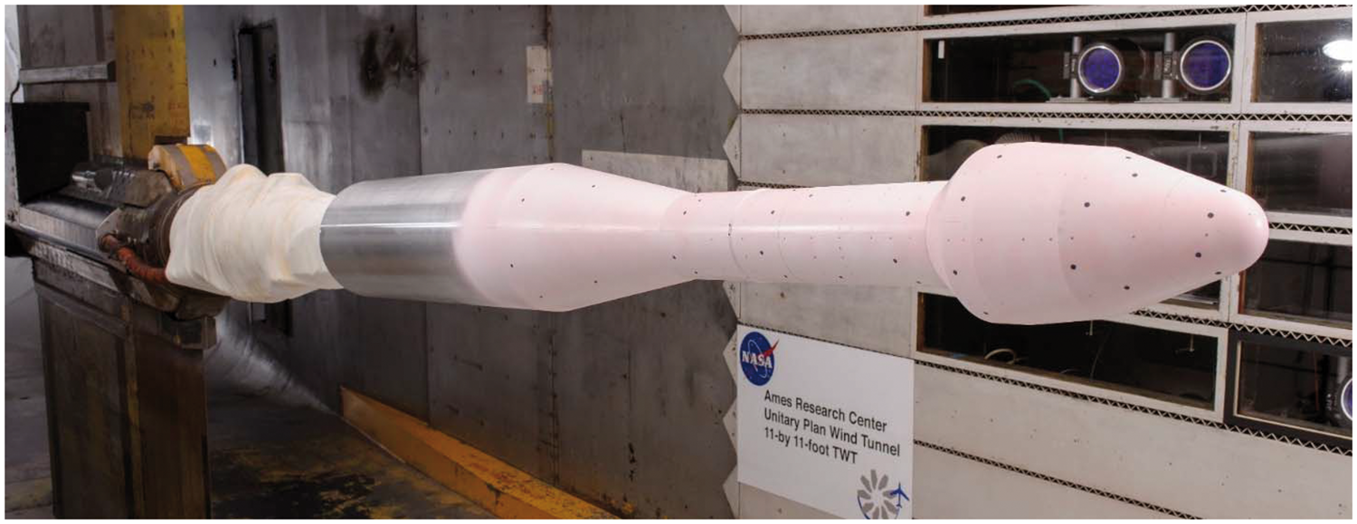

Experimental procedure

The present test was conducted in the transonic 11-by-11 ft test section of the Unitary Plan Wind Tunnel at NASA Ames Research Center. Detailed data are available for Mach numbers of 0.6, 0.8, 0.85, 0.92, 1.025, and 1.1 for at least three angles of attack of α = −4 °, 0 °, and 4 °. Additional data for a combination of angle of attack α and sideslip angles β are also available for a limited Mach number conditions. Finer Mach number increments were tested for α = 0 ° and β = 4 ° attitude over 0.6 ≤ M ≤ 1.2 range. In addition to the unsteady pressure sensors, the launch vehicle model was instrumented with accelerometers, a custom built six-component strain gauge balance, and was coated with an unsteady pressure-sensitive paint. A detailed description of the experiment and all instrumentations can be found in Schuster et al.¹² The Transonic Wind Tunnel has a test section of dimension 11 ft (high) × 11 ft (wide) × 22 ft (length) and is capable of simulating static pressure conditions at different altitudes (variable density, Reynolds number). The test section walls have lengthwise slots for shock cancellation and for applying wall suction. A particularly desirable feature of the wind tunnel is the optical access on all four walls via segmented windows that are separated by the wall slots.

The model was an exact replica of that of Coe and Nute.¹¹ Figure 2 shows a schematic and various nomenclatures used in the text. The topmost part represents the payload fairing and has multiple sections of progressive area increase followed by a sharp drop at the frustum to match the dimension of the second stage. The conical sections of the payload fairing are conducive to an ease in manufacturing of the large panel structures. Various modern vehicles use a smother tangent-ogive configuration which is subjected to similar aerodynamic phenomena. The frustum in effect creates a backward-facing step causing flow separation. Various dimensions of the frustum have been parts of multiple studies¹^–^3,11 to avoid excessive flow-induced vibration. The second stage merges with the booster stage of the vehicle through an adapter. Some current launch vehicles that use strap-on boosters typically maintain a constant diameter between the first and the second stages; however, the essential flow physics of a large separated zone on the second stage is still present.

Figure 2.

Schematic of the model. Red circles show the locations of the dynamic pressure transducers used by Coe and Nute and the blue lines indicate the locations of circumferential groups in the present test. The group name and the associated number of sensors are indicated.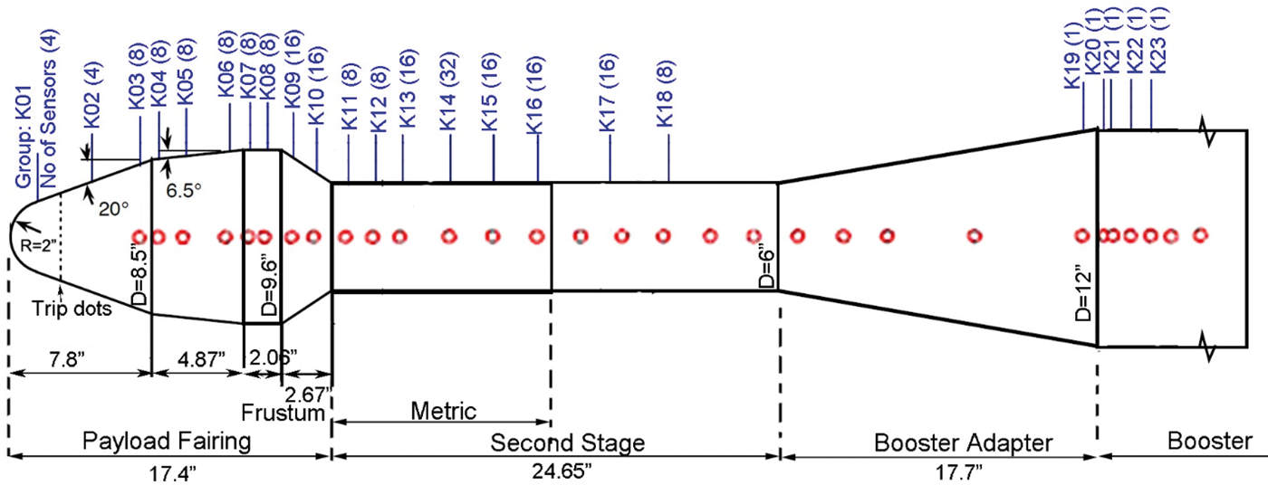

Only a limited number of pressure measurements along a line were made in the original study by Coe and Nute; the present model used 216 flush-mounted, 0.072 in diameter Kulite™ sensors (13 of which failed after installation). The sensors were grouped in circumferential rings, marked K01–K23 (Figure 2), and the individual sensors in each group were marked by an extension. For example, sensors located at station 01 and at circumferential angles of θ = 0 °, 90 °, 180 °, and 270 ° were marked, respectively, K01-01, K01-02, K01-03, and K01-04. The number of sensors in each ring was varied (per the number in parenthesis in Figure 2); the exact locations were reported by Schuster et al.¹² A line of sensors was placed at the same location as that of the Coe and Nute study. The latter lacked any sensor at the nose cone which, for the present experiment, was instrumented with two rings of sensors—K01 and K02—each containing four Kulites™. There were an additional 16 circumferential rings—K03–K18—on payload fairing and the second stage of the model. The booster and the downstream half of the second stage had only a row of sensors along the 0 ° azimuthal direction. The differential sensors were a mix of 5 and 15 psi range. The reference tubes were connected to a common plenum, and the amplifier outputs were DC coupled. Output from each sensor was digitized using a 24-bit, sigma-delta converter at a sampling rate of 100,000/s.

The experimental uncertainty associated with the dynamic pressure data presented in this paper is expected to be small. The random error estimated by repeating test points was found to be <1% of the quoted values for the overall fluctuation levels. This is within the maximum uncertainty of ±1% specified by the vendor. The drift in the sensor calibration is typically <1%. Another source of uncertainty in the dynamic pressure measurement was associated with the mounting of some of the Kulite™ sensors. The model was coated with pressure-sensitive paint which required individual sensors to be protected by small dots of tapes during the application of the paint. The dots were removed before the test, but the paint was found to make a couple of microns high ridge around some sensors. This installation issue may have introduced small yet undetermined error at the high frequency end of the spectra.

The facility Schlieren/shadowgraph system was in the classic Z-configuration and consisted of a high-powered LED source, two light collimating 4 f diameter mirrors, optical quality test section glass, digital cameras with associated optics, and data systems. For this entry shadowgraph (no knife edge) images were taken, as it was more sensitive to the gradients produced by shock wave and fine-scale turbulence. For the present application, a single Phantom v2010 high-speed camera was used to capture shadowgraph images of the upper half of payload fairing and the second stage. Typical acquisition parameters were 40,000 frames/s, six microsecond exposure times, with 5300 frames collected at each test condition. Shadowgraph images were only acquired for an angle of attack α = 4 °. Optical access at the 11-by-11 ft test section is limited by the rectangular window frames and slotted wall baffles (see Figure 1). Additional space limitations allowed for imaging only of the upper half of the model.

Recently, Garbeff et al.¹⁵ processed the sequence of shadowgraph images from the high-speed camera to provide a qualitative description of turbulent fluctuations over the model. The time history of light intensity variation for each pixel I(x, y, t) from all 5300 frames was extracted, and the standard deviation σ_I(x, y) was calculated in the time dimension

σ_{I} (x, y) = \sqrt{\frac{1}{5300} \sum_{i = 1}^{i = 5300} (I - \bar{I})}

(1)

Here x and y are pixel coordinates, and the overbar represents a time average. Since the variation of the light intensity corresponds with the density variation, images of the distribution of σ_I were found to identify the high turbulence regions over the model. Such distributions will be shown later in this paper.

Data acquisition system used by Coe and Nute

The present test used modern pressure sensors, digital electronics, and a 24-bit sigma-delta analog-to-digital converter that had flat frequency response over the entire 50 kHz frequency range. However, the sensors that Coe and Nute used had a linear response over a limited frequency range of 1 kHz. Coe and Nute mostly presented the rms of pressure fluctuations and a small number of spectra. For the former they used an analog rms meter which band-pass filtered the analog output of each sensor. Figure 3 is a copy of the frequency response function of the filter shown in their paper. For a meaningful comparison, the present data also needed to be similarly filtered. A simple digital filter was created by calculating narrowband power spectra from the time series data. The power spectral density (psd) values between 5 and 1000 Hz were used to calculate the rms pressure fluctuations as follows

σ_{p - filt} = \sqrt{\sum_{f_{i} = 5}^{f_{i} = 1000} psd (f_{i})}

(2)

Figure 3.

(Solid line) Amplitude response of the band-pass filter used by Coe and Nute; (chain line) that for the present comparison.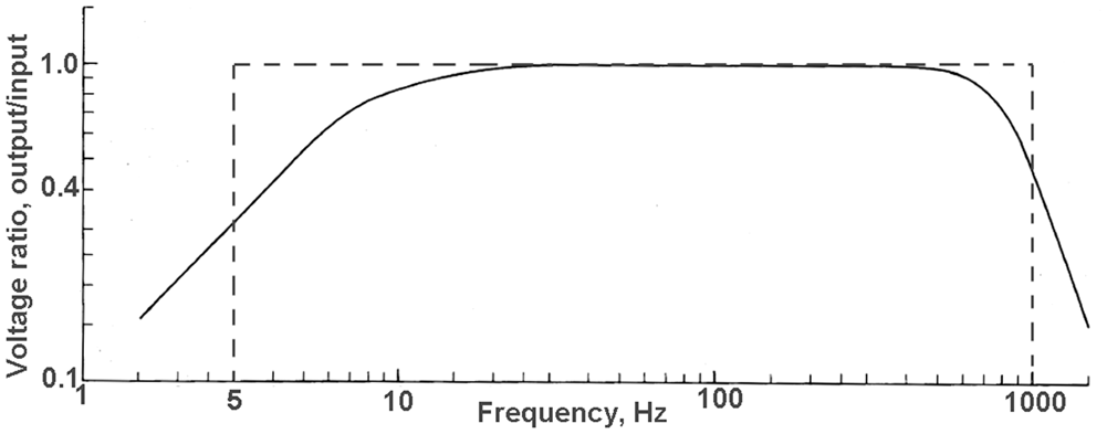

To determine the spectra of pressure fluctuations, Coe and Nute¹¹ and Coe¹⁶ used analog tapes to record a filtered and amplified signal from the microphone sensors. The tape recorder also recorded a known AC calibration signal to characterize the gain in the recorder data system. The analog tapes were then played back and the output passed through an analog power spectrum analyzer to a recording potentiometer. The spectral data had a limited frequency band of f ≤ 500 Hz.

Results and discussion

The series of shadowgraph images of Figure 4 provides insight into the primary flow phenomena. The central flow feature of the hammerhead model is a flow separation at the frustum part of the payload fairing. The separated shear layer reattaches some distance downstream on the second stage creating large fluctuations in local static pressure. At the lowest M = 0.6 no shock waves are formed. The sharp boat tail angle at the frustum pinned the separated shear layer which impinged on the second stage creating high levels of pressure fluctuations around the impingement location. This flow phenomenon was present at all Mach numbers. The payload fairing was subjected to local shock and separation events in transonic flow. At M = 0.8, local supersonic zones set in at the two locations (the junction between the two conic sections and at the second cone–cylinder junction) associated with the sudden area increase on payload fairing. Each of these zones was terminated by a normal shock. The shock–boundary layer interactions were found to create large spikes in pressure fluctuations. A small increase in the free-stream Mach number to M = 0.85 caused the supersonic bubble to grow and pushed the normal shock downstream on the fairing. At M = 0.92, supersonic flow covered almost the entire payload fairing except for the frustum; the normal shocks coalesced into one and stood at the upstream end of this neck-down. Further increase of the free-stream Mach number to 1.05 made the payload fairing shock free. Limited by the 4 ft diameter mirrors, the shadowgraph images did not cover the downstream booster part of the model. This region was also subjected to local transonic shock waves.

Figure 4.

Shadowgraph images of the upper half of the model at indicated Mach numbers. (a) M = 0.6, α = 4°; (b) M = 0.8, α = 4°; (c) M = 0.85, α = 4°; (d) M = 0.92, α = 4°; (e) M = 1.05, α = 4°; (f) M = 1.2, α = 4°.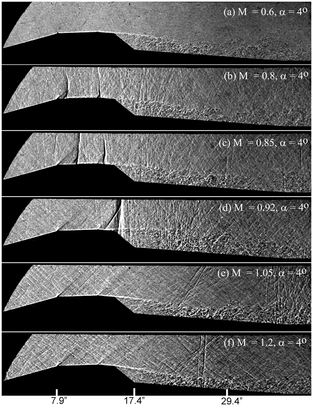

The composite images of Figure 5 further illustrate the origins of the high level of pressure fluctuations. Each composite image is made up of three parts: two of which are from the high-speed shadowgraph camera, and the third from the data collected from the dynamic pressure sensors. The single frames from the camera provide snapshots of the flow features, and the 2D plots of standard deviation of the light fluctuations σ_I provide insight into the unsteadiness in the airstream. Note that the same color scales were used among all σ_I and Cprms cases. While it is desirable to measure turbulence fluctuations in most wind tunnel tests, experimental techniques that can provide quantitative measurements in transonic tunnels are few (particle image velocimetry, Rayleigh scattering, etc.) and are costly to setup in large tunnels. The high-speed shadowgraph (and Schlieren) provides a cheap alternative, although the actual physical quantity measured is obscure—shadowgraph images produce path-integrated changes of a derivative of density. Nonetheless, the σ_I plots show the growth of the separated shear layer from the top of the payload fairing and impingement on the second stage. The third part shows distribution of Cprms on the model surface. For this purpose, the standard deviation of pressure fluctuations σ_p (over the entire frequency band) measured by the sensors was calculated and then normalized by the free-stream dynamic pressure q: Cprms = σ_p/q. The Cprms values were distributed on a wire mesh model of the test article using a “nearest neighbor”-based interpolation scheme. Taken together, Figure 5 combines the off-body shadowgraph measurements with the on-body pressure transducer measurements, providing a more complete picture of the flow field.

Figure 5.

Composite of shadowgraph image, rms of light intensity fluctuations calculated from the high-speed shadowgraph images, and distribution of Cprms measured by dynamic pressure sensors at indicated three Mach numbers. (a) M = 0.6, α=4°; (b) M = 0.8, α=4°; (c) M = 1.1, α=4°.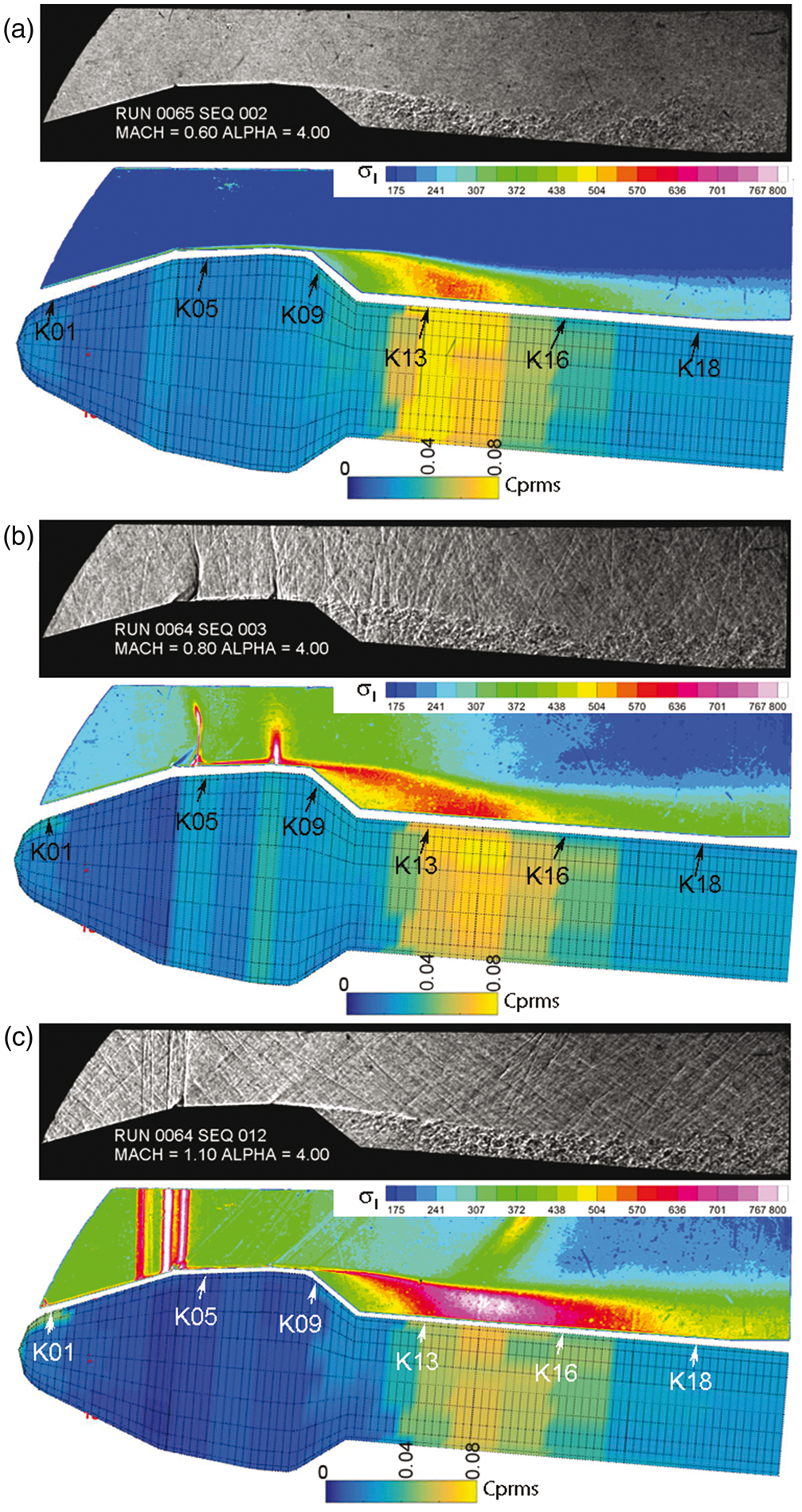

An examination of the composite images shows that the pressure fluctuations are mostly low on the payload fairing except when transonic shocks are present (Figure 5(b)) which causes a thickening of the boundary layer and an increase in the unsteadiness. The first shock sets up the high level of fluctuations which are then amplified by the second. The unsteady motion of the entire shock front is captured by the high level of σ_I around individual shocks. The high level of fluctuations along vertical lines (on payload fairing) in Figure 5(c) is due to the “window shock,” i.e. the intersection of the model shock with the test section wall, which did not affect the flow around the model. At M = 1.1 the steep oblique shock formed at the nose of the model may have partially reflected from the tunnel and have manifested in the shadowgraph. Recall that shadowgraph shows path-integrated fluctuations over the width of the entire test section.

Figure 6 shows narrowband power spectra from various regions of the model. The low-frequency rich spectra are typical of separated–reattached flows. It is known that the pressure fluctuations in such low-frequency bands are also capable of exciting various vibrational modes of the panels and shells that makeup the outer body of a space vehicle. There lies the need to define “forcing function” for vibro-acoustics analysis via wind tunnel tests. A closer look into the spectra shows that there are no discrete features except at the frequency bands affected by the wind tunnel background noise. Unlike low subsonic and supersonic wind tunnels, the free-stream turbulence fluctuations are much higher in transonic tunnels due to the presence of the wall slots (or holes) which are necessary to reduce shock reflection and to minimize blockage. Such slots create sharp tones or narrow humps that can be identified in the data collected from empty test section operation. Such humps (pointed out in Figure 6) are prominent in the regions of the model subjected to low levels of pressure fluctuations and are swamped at locations subjected to higher levels.

Figure 6.

psd of pressure fluctuations from indicated sensors shown in Figure 5, and at the same M, α conditions. (a) M = 0.60; (b) M = 0.80; (c) M = 1.10.

Another feature to point out is the relatively high level of pressure fluctuations at the nose of the model. This is more prominent on the leeward side of the model in Figure 5(c). Power spectrum from the sensor K01-01 located at the nose shows rich content in Figure 6(c); that from the next sensor K02-02 (not shown) is less energetic; and the very low level, close to the tunnel background, measured by the sensor K05-05 implies a relaminarization of the boundary layer. Trip dots were applied on the model downstream of the sensor group K01 to expedite boundary layer transition (Figure 2). The high level of fluctuations ahead of the trip dots implies the presence of a laminar separation bubble at some Mach number conditions. Infrared camera images collected during the test showed transition forward of the trip dots.¹²

Space–time correlation

In addition to the overall levels and power spectra of pressure fluctuations, the vibro-acoustics analysis procedures require information on space–time correlation of fluctuations. Such correlations are used to provide measures of convective velocity and correlation lengths. The normalized correlation coefficient r between two spatial points separated by Δx and Δθ is given as

r (Δ x, Δ θ, τ) = \frac{1}{τ} \frac{1}{p_{rms} (x, θ) p_{rms} (x + Δ x, θ + Δ θ)} \int_{0}^{T} p (x, θ, t) p (x + Δ x, θ + Δ θ, t + τ) d t

(3)

Here T is the time duration of the signal. Figure 7 shows two sets of space–time correlations between pairs of sensors separated in the axial direction. For each set one of the sensors in all pairs, marked as the reference sensor, was kept fixed. Correlating the reference sensor with itself results in the auto-correlation, which as expected has a peak value of unity at zero time delay. Figure 7(a) shows auto- and cross-correlation plots for pairs located on the second stage, and Figure 7(b) for pairs on the payload fairing. Note that for all correlation plots, sensors at the azimuthal θ = 0° position were used. The additional tail “−01” in the sensor number is omitted for brevity.

Figure 7.

Space–time correlation of pressure fluctuations measured by indicated sensor pairs and at indicated flow conditions; (a) separation–reattachment zone on second stage, M = 0.8, α=4°; (b) payload fairing, M = 0.8, α=4°.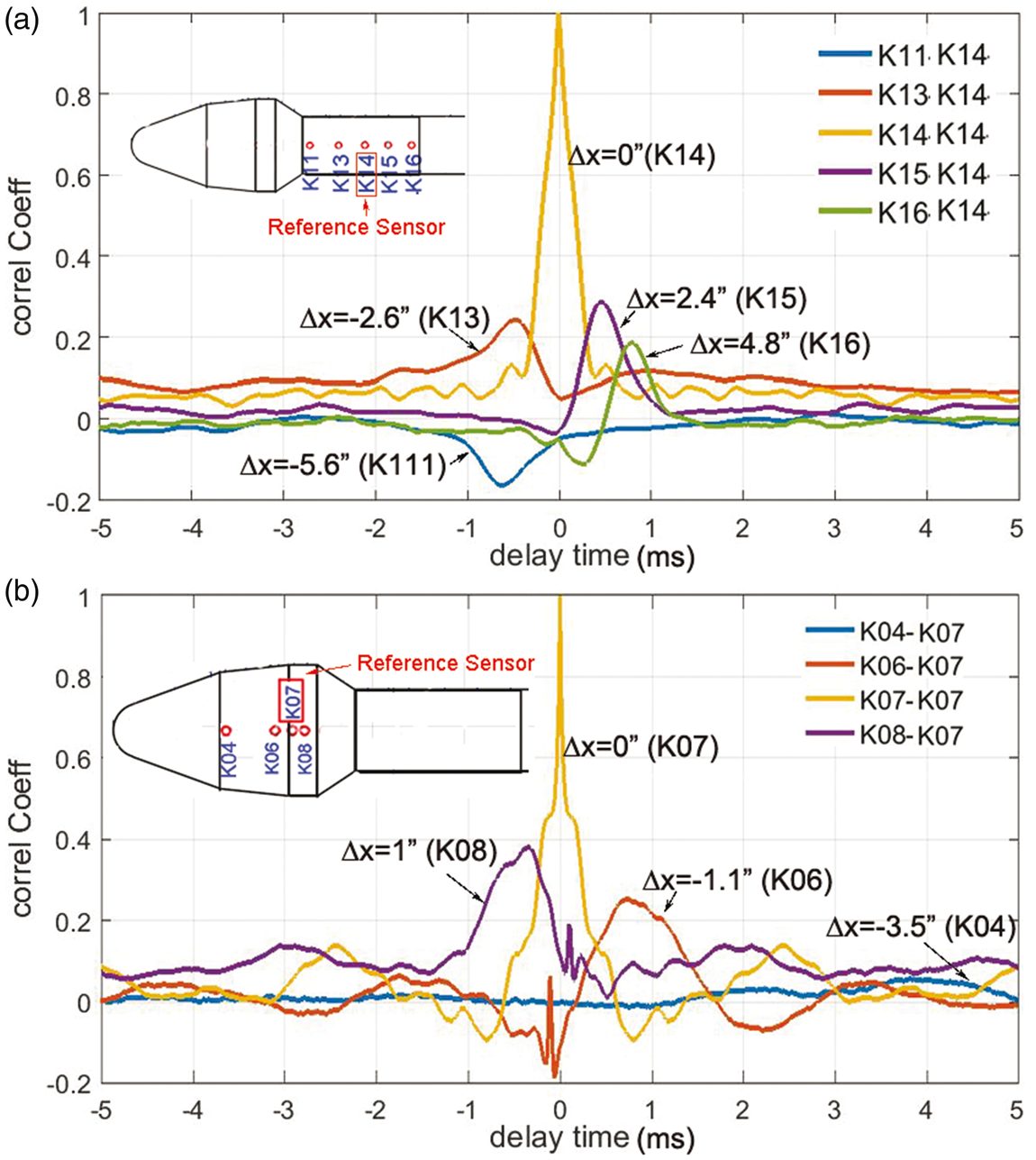

Examination of the correlation plots shows that each has a local peak that appears at a delay time τ which can be used as a measure of the convection velocity of pressure fluctuations. For a fixed separation Δx, the time delay, τ, that produced the peak in correlation provides the convection velocity Uc = Δx/τ. For the second stage (Figure 7(a)) an average convection velocity, normalized by the free-stream velocity is calculated to be Uc/U = 0.55 (this number excludes the K11–K14 pair which indicate complex, perhaps upstream, propagation). The data from the payload fairing (Figure 7(b)), however, show a striking difference—peaks in correlation coefficient appear in negative delay times for positive spatial separation between sensor pair and vice versa. Physically this implies that the local pressure fluctuations propagate upstream on the payload fairing. The normalized convection velocity was found to vary between −0.3 ≤ Uc/U ≤ −0.1 depending on the pair of sensors used for calculation.

To further investigate this phenomenon of upstream propagation, correlation coefficients from the same pairs of sensors are plotted for M = 0.92 and 1.03 in the two parts of Figure 8. The former (Figure 8(a)) shows even higher levels of correlation and significant upstream propagation; the latter however indicates a sharp drop with the arrival of supersonic regime. Recall that at M = 0.8 and 0.92 (Figures 7(b) and 8(a)) local shock waves are formed on payload fairing while such shocks are washed away when the free stream exceeds the speed of sound. It is believed that the local transonic shock waves create significant coupling of pressure fluctuations on the payload fairing with that of the separated flow region on the second stage. Although the transonic shocks are preceded by a supersonic zone, low-frequency pressure fluctuations are still capable of upstream propagation through the viscous sublayer and inner layer of the boundary layer.¹⁷ The presence of the local separation under the shock waves may have improved the propagation path. Note that the unsteady PSP data from this test, reported earlier,¹³ also confirmed the upstream propagation of the pressure fluctuations at transonic Mach numbers. Data from a wind tunnel test of a scaled model of the Vega vehicle⁹ also showed upstream propagation of some parts of the pressure fluctuations. Such a coupling can generate large forces and structural deflection of the entire launch vehicle stack. It is worth recalling that nearly a half century ago the hammerhead family of space vehicles were scrutinized to mitigate excessive buffet forces encountered by certain configurations.¹^–^3,11 Recommendations for the frustum angle, ratio of the payload diameter to that of the second stage, length of the second stage to the fairing diameter, and other similar parameters were generated to avoid the excessive unsteady forces. These parameters are widely used in present vehicle designs. The current model configuration is one that was recommended by those studies. The present observation indicates that for other buffet-prone hammerhead geometries, an even stronger coupling could have been present between the second stage and the payload fairing, leading to excessive lateral forces and limit cycle oscillation at small angles of attack.

Figure 8.

Space–time correlation of pressure fluctuations measured by indicated sensor pairs on the payload fairing at (a) M = 0.92, α=4° and (b) M = 1.03, α = 4°. Similar data from M = 0.8 is shown in the figure above.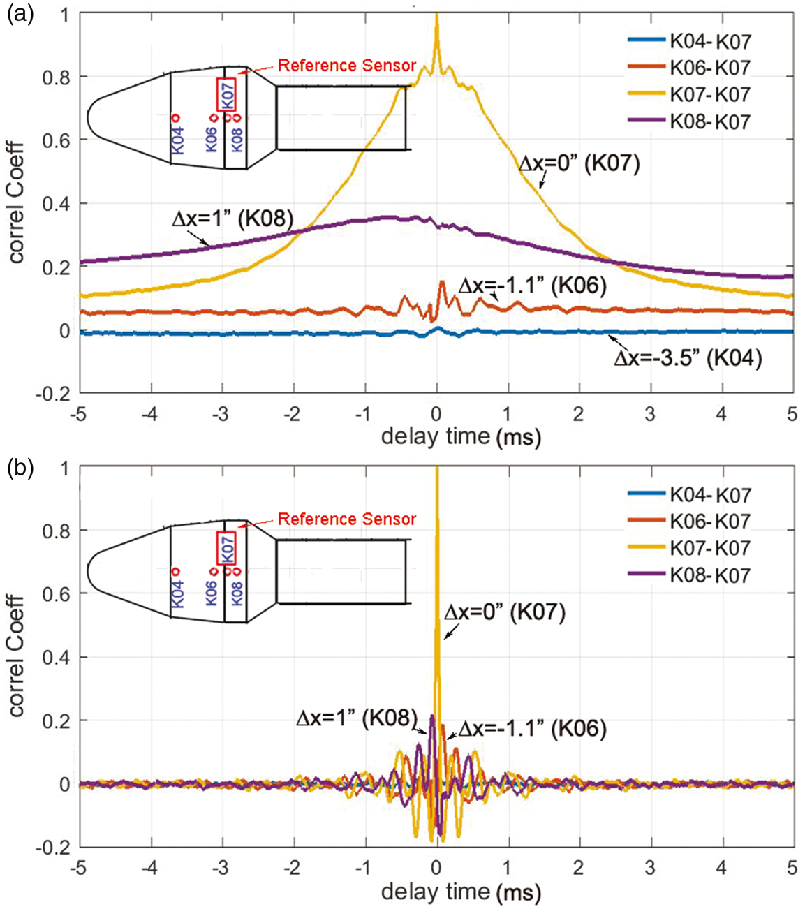

Comparison with Coe

A large portion of unsteady data presented by Coe and Nute was in the form of Cprms distribution along the axial direction for a set of Mach number conditions. Figures 9 and 10 show a set of comparisons where the current data are shown via blue and red lines (Coe and Nute data shown in black lines). The blue data were calculated from the full frequency band, 1 Hz to 50 kHz, while the red data used a 5 Hz to 1 kHz filter to duplicate the limited frequency range of Coe and Nate (Figure 3). As expected, the band-pass data provide a better match with the Coe and Nute results. The comparisons are in general reasonable. Interestingly, the comparisons improved with Mach number. The present band-pass Cprms values were slightly higher than those measured by Coe and Nute, but the difference diminished with increasing Mach number. Another difference was in the absolute values of the sharp peaks caused by the localized transonic shocks. Coe and Nute changed the tunnel Mach number in very small increments to position the shock waves on the top of a sensor to capture the local peaks. No such attempts were made in the present work; data from the unsteady pressure-sensitive paint were expected to capture the local peaks.¹³

Figure 9.

Comparison of Cprms measured in the current test and by Coe and Nute for (a) M = 0.6, and (b) M = 1.08 and for the three indicated angles of attack. Individual sets of plots are vertically separated by 0.1.

Figure 10.

Comparison of Cprms measured in the current test and by Coe and Nute for indicated Mach numbers and for α = 0°. Individual sets of plots are vertically separated by 0.1.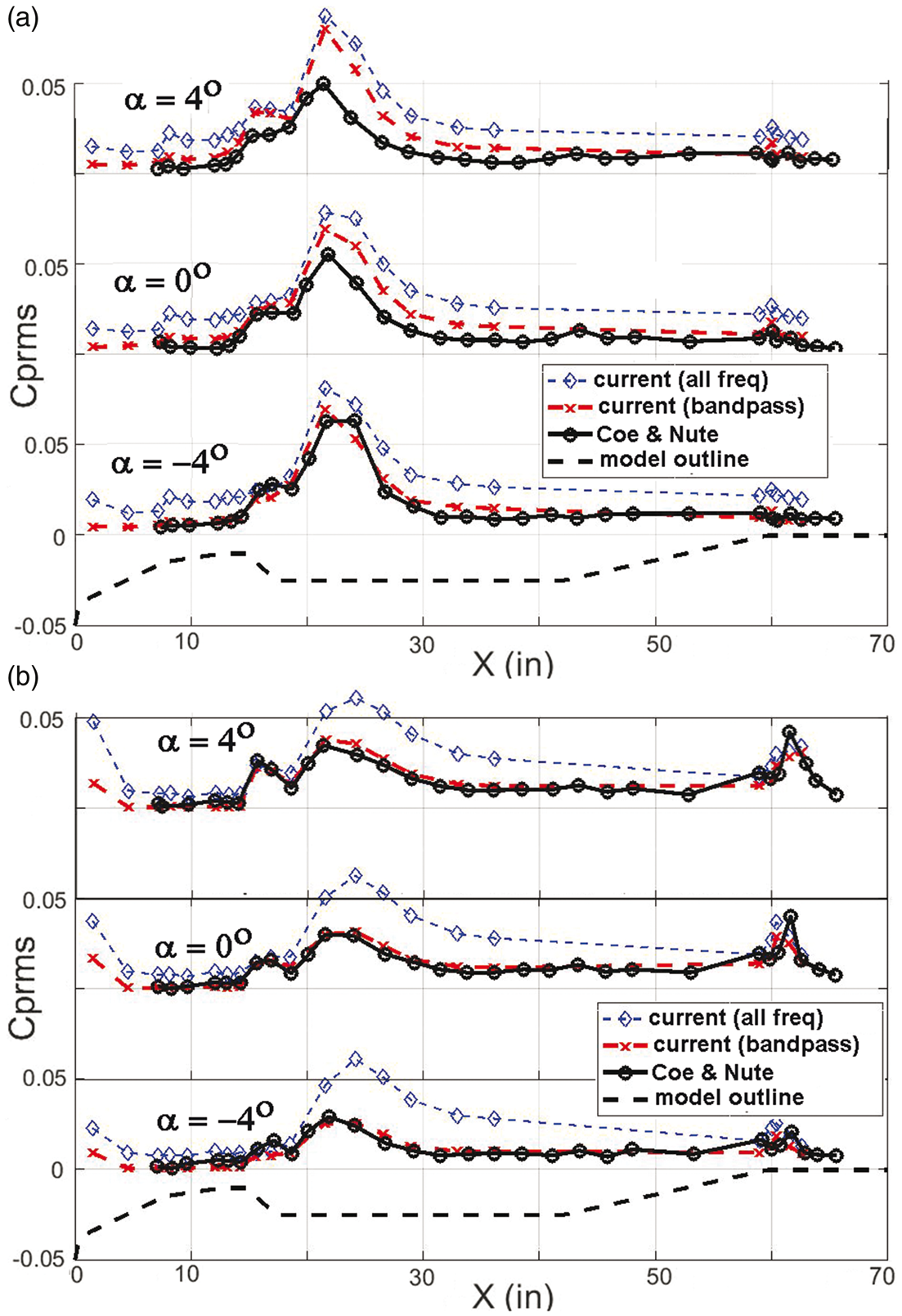

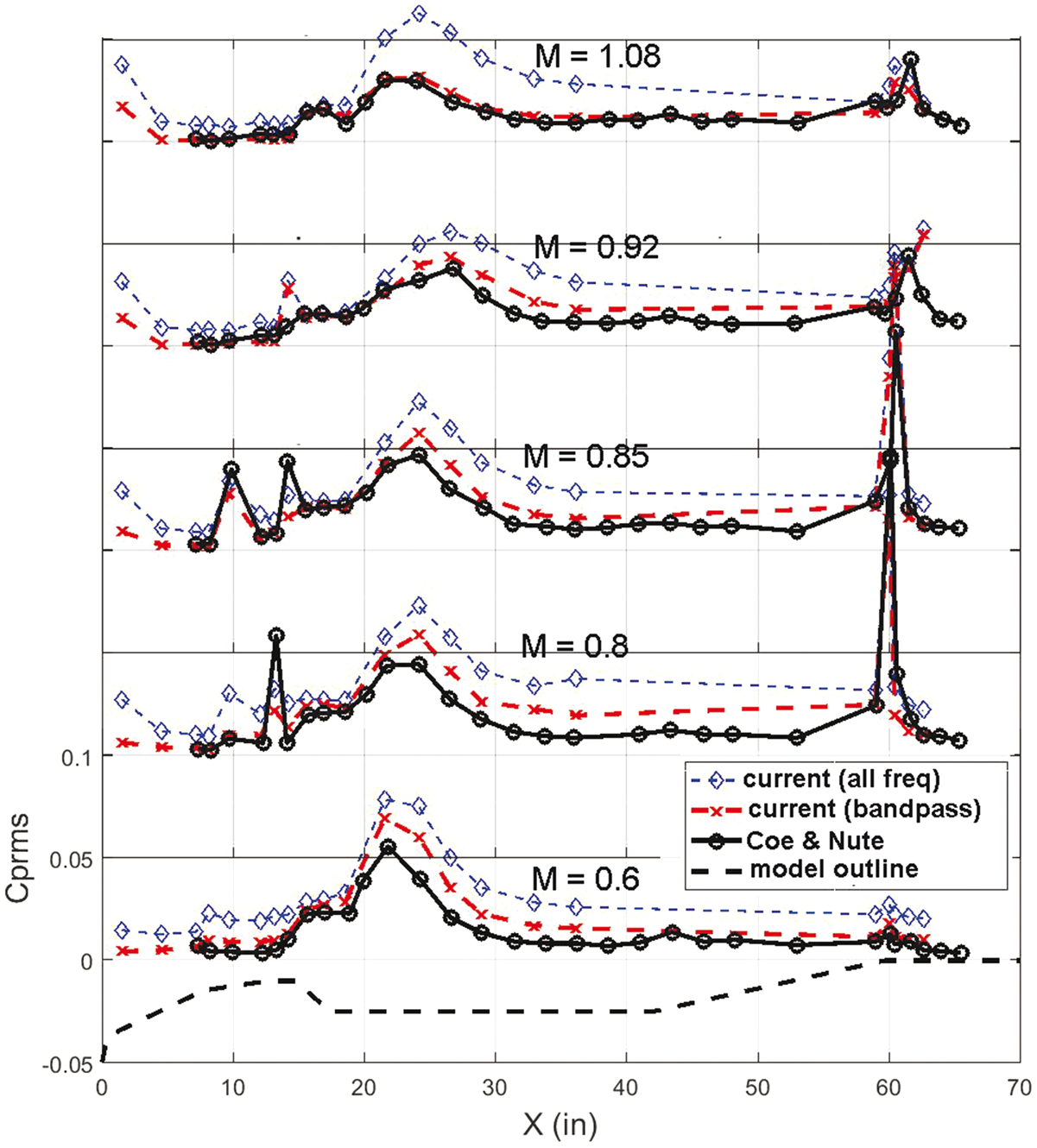
A closer look into the Cprms distribution of Figure 10 shows a few interesting features. First, the peak Cprms progressively decreased with increasing Mach number, this is attributed to the compressibility effect which lowers the turbulent fluctuations with increasing M. The second is the location of the peak fluctuations at the reattachment zone on the second stage. The peak moved downstream until M = 0.92 and then shifted back upstream at M = 1.08. An examination of the shadowgraph photographs of Figure 4 revealed the cause of this movement. The local shock waves that formed on the top of the fairing lifted the separating shear layer on the frustum. The lift is the most prominent at M = 0.92. Such a lifting of the shear layer increased the extent of the separated flow and moved the reattachment point downstream. Since the location of the peak fluctuations is associated with the reattachment point, the maxima in fluctuations are also pushed downstream. When the local shocks disappeared with an increase in Mach number, so did the upward curving of the shear layer, and the reattachment point and the peak location of pressure fluctuations retracted back upstream.

Figure 11 shows a comparison of power spectra measured in the present test and that by Coe and Nute. One of the necessary steps was to account for the difference in the dynamic pressure q between the two tests. The magnitude of pressure fluctuations is known to be proportionate to the free-stream dynamic pressure: p′∝ q. Therefore, the psd is proportional to q²

psd \propto q^{2}, i . e . \frac{ps d_{Coe}}{ps d_{present}} = (\frac{q_{Coe}}{q_{present}})^{2}

(4)

Figure 11.

Comparison of power spectra from four different (indicated) dynamic pressure sensors between the present test and that of Coe and Nute; M = 0.95, α = 0°. PSD: power spectral density.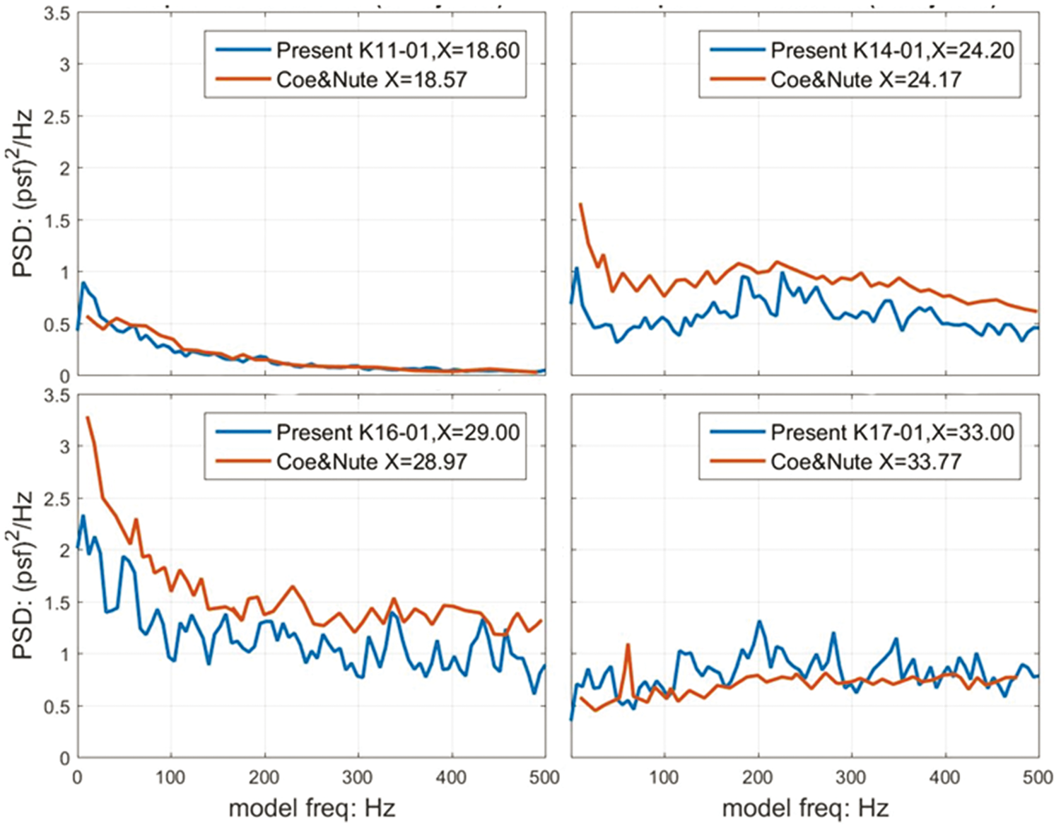

Since dynamic pressure is related to the ratio of specific heat γ, the tunnel static pressure P and Mach number: q = ½ γPM². Both γ and M were constants between the two wind tunnels, therefore following holds

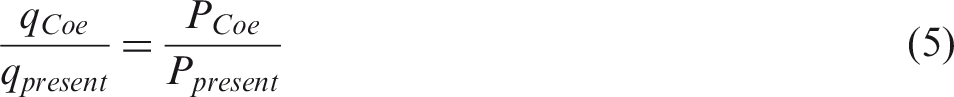
\frac{q_{Coe}}{q_{present}} = \frac{P_{Coe}}{P_{present}}

(5)

Coe and Nute performed their test in the old (now demolished) 14 ft Transonic Wind Tunnel. They did not report the dynamic pressure q but reported the operating Reynolds number. For the particular M = 0.95 condition the Reynolds number per foot was Re_Coe = 4.15 × 10⁶. The present data were collected for Re_present = 3 × 10⁶. Reynolds number per foot is defined via free-stream density ρ, velocity U, and dynamic viscosity μ: Re = ρU/μ. Besides the difference in the Reynolds number one also needs to know the free-stream temperature to determine the difference in the dynamic pressure. In absence of such information, it was assumed that the tunnels operated with nearly same temperature conditions, leading to the following inference

\frac{q_{Coe}}{q_{present}} = \frac{{Re}_{cos}}{{Re}_{present}} = \frac{ρ_{Coe}}{ρ_{present}} = \frac{P_{Coe}}{p_{present}}

(6)

The above relationship allowed for the following adjustment of the psd levels measured from the present test

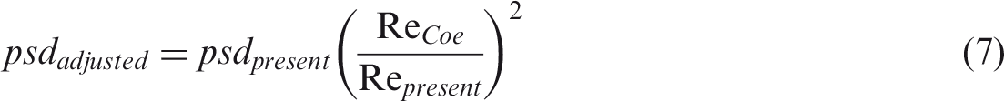
ps d_{adjusted} = ps d_{present} (\frac{{Re}_{Coe}}{{Re}_{present}})^{2}

(7)

The adjusted power spectra are compared with data presented by Coe and Nute in Figure 11 and are found to be in reasonable agreement. The differences can be attributed to the assumptions mentioned above and the differences in the measurement devices between the two tests. There is an inconsistency between the spectral data of Figure 11 and the rms levels shown in Figure 10. Spectra from the present work at X = 24.2 and 29.0 fall below those of Coe, yet the rms levels are uniformly above those of Coe. Indeed, this may be a problem with the lack of information regarding dynamic pressure in the original paper.

Conclusion

A series of studies in 1960s by Coe and others on axisymmetric models demonstrated the importance of unsteady aerodynamics for aeroacoustics and the buffet environment of space vehicles. The conclusions gained from these studies resulted in significant contributions toward the design of modern launch vehicles. The present test was undertaken to advance experimental tools, to provide a complete picture of pressure fluctuations which can be used to advance buffet and vibro-acoustics analysis capabilities, and to validate computational codes. The model under study was a generic “hammerhead” shape, originally studied by Coe and Nute (model 11 in their study). In spite of more than half a century of separation, careful considerations of the differences in instrumentation and also the difference in the wind tunnel conditions led to fairly good agreements between the present and the past data. It is also demonstrated that the large database can produce hitherto unknown insights. For example, space–time correlation of surface pressure fluctuations demonstrated coupling between the shock waves formed on the payload fairing and the large separation–reattachment flow on the second stage of such vehicles. Such couplings are capable of producing large forces and vibratory environments.

Footnotes

Acknowledgements

As the PhD thesis advisor of the first author, Prof. Dennis K. McLaughlin guided him during the formative years. The technical staff at the Ames Wind Tunnel Division was critical in all aspects of this test. The Editor-in-Chief, G. Raman, served as the sole independent editor for this paper.

References

Cole HA Jr, Erickson AL and Rainey AG. Buffeting during atmospheric ascent. NASA SP-8001, May 1964, revised 1970.

Ericsson

. Unsteady flow separation can endanger the structural integrity of aerospace launch vehicles. J Spacecr Rockets 2001; 38: 168–179.

Robinson RC, Wilcox PR, Gambucci BJ, et al. Dynamic response of a family of axisymmetric hammerhead models to unsteady aerodynamic loading. NASA TN D-4504, 1968.

Jones GW and Foughner JT Jr. Investigation of buffet pressures on models of large manned launch vehicle configurations. NASA technical note D-1633, 1963.

Hanly RD. Surface pressure fluctuations associated with aerodynamic noise on the space shuttle launch configuration at transonic and supersonic speeds. In: Seventeenth structures, structural dynamics, and materials conference, King of Prussia, PA, USA, 1976. https://doi.org/10.2514/6.1976-1527.

Herron AJ, Crosby WA and Reed DK. Overview of the space launch system ascent aeroacoustic environment test program. AIAA paper 2016-0543, 2016.

Troclet B, Depuydt M and Gonzalez P. Experimental analysis of the aerodynamic noise on the Ariane 5 launch vehicle upper part. In: Conference proceeding “Ariane 5 structures and technologies,” 1993, pp.515–526. France: CNES.

Gibson

Janssen

Bradford

et al.

Overview of the development of dynamic environment for Atlas V launch vehicles. J Spacecr Rockets 2004; 41: 779–786.

Camussi

Guj

Imperatore

et al.

Wall pressure fluctuations induced by transonic boundary layers on a launcher model. Aerosp Sci Technol 2007; 11: 349–359.

10.

Murman SM and Diosady LT. Simulation of a hammerhead payload fairing in the transonic regime. AIAA paper 2016-1548, 2016.

11.

Coe CF and Nute JB. Steady and fluctuating pressures at transonic speeds on hammerhead launch vehicles. NASA TMX-778, 1962.

12.

Schuster DM, Ross JC, Panda J, et al. Investigation of unsteady pressure-sensitive paint (uPSP) and a dynamic loads balance to predict launch vehicle buffet environments. NASA NESC report TI-14-00962, 2016.

13.

Panda J, Roozeboom NH and Ross JC. Wavenumber-frequency spectra of pressure fluctuations on a generic space vehicle measured via unsteady pressure-sensitive paint. AIAA paper 2017-1406, 2017.

14.

Ngo C, Powell J and Ross J. Inverse force determination on a small scale launch vehicle model using a dynamic balance. AIAA paper 2017-1405, 2017.

15.

Garbeff TJ II, Panda J, Ross JC, et al. Experimental visualizations of a generic launch vehicle flow field: time-resolved shadowgraph and infrared imaging. AIAA paper 2017-1403, 2017.

16.

Coe CF. Steady and fluctuating pressures at transonic speeds on two space-vehicle payload shapes. NASA TMX-503, 1961.

17.

Schneider

. Upstream propagation of unsteady disturbances in supersonic boundary layers. J Fluid Mech 1974; 63: 465–485.