
Abstract
Noise source imaging based on phased array measurements is an essential tool in the aeroacoustic analysis of new nozzle designs, especially at full-scale. This investigation aims to assess the capability of a deconvolution-based beamforming technique to accurately estimate the changes in noise sources for model-scale heated military jets when fluid inserts are used for noise control. This goal is achieved by performing well-validated Large Eddy Simulations (LES) to complement the experimental measurements. The LES data is segregated into its hydrodynamic, acoustic and thermal components using Doak’s Momentum Potential Theory (MPT). The near-field MPT-derived components are subjected to Spectral Proper Orthogonal Decomposition (SPOD) to compare with the frequency-dependent noise source maps obtained directly from experiments. It is shown that fluid inserts alter the naturally occurring Kelvin-Helmholtz (K-H) instability in the jet shear layer, which leads to a change in the directivity of the noise radiated in the near-field. The upstream shift in the noise source distribution resulting from the modified K-H instability is accurately captured by the deconvolution-based source imaging technique using just the far-field measurements. These changes in source locations as a function of frequency are documented.
Introduction
Supersonic, high-temperature jets exhausting from tactical aircraft engines create hazardous noise environments that affect the health and performance of military personnel working in the vicinity of these aircraft. They are also a source of annoyance in communities close to naval airbases and military training routes. According to a report in 2010 by Doychak, 1 the U.S. Department of Veterans Affairs spends hundreds of millions of dollars each year for hearing loss cases and noise complaints. A decade later, this number is almost certainly significantly higher. This motivates investigations into various noise reduction technologies for existing and next-generation military aircraft.
An accurate estimation of noise source characteristics is essential in assessing novel nozzle designs and noise reduction concepts. However, direct measurement of flow parameters in the jet near-field is extremely challenging and cost-prohibitive in full-scale tests due to the heated, turbulent nature of the flow-field. Therefore, source localization techniques typically rely on microphone measurements in the acoustic field to model a presumed form of noise source distribution that best fits the microphone data. Notably, Tam et al. 2 performed auto- and cross-correlations of far-field pressure measurements from both subsonic and supersonic jets to argue in favor of the existence of the now widely-accepted two-source model of jet noise. These findings were further corroborated by using an elliptic mirror microphone 3 to estimate noise source distributions from fine-scale and large-scale turbulence. More sophisticated noise imaging techniques involve the use of polar-correlations4–6 and phased arrays7–10 to estimate frequency-dependent noise source maps in both model-scale jets and full-scale engines.8,11–14
The goal of the present investigation is to assess the capability of a deconvolution-based source imaging technique 15 to accurately estimate the changes in the frequency-dependent noise source distributions in heated over-expanded military-style jets when fluid inserts 16 are used for noise control. A fluid insert is a linear array of small diameter injectors that blow a small fraction of the bypass air into the diverging section of a converging-diverging nozzle. The use of fluid inserts has been shown to be successful in reducing supersonic jet noise in both upstream and downstream directions at different nozzle sizes 17 and operating conditions. 18
This paper describes model-scale experiments carried out in the Pennsylvania State University’s high-speed aeroacoustics facility, both with and without fluid inserts. Noise source maps are generated for each jet using far-field measurements. The use of the deconvolution-based algorithm is motivated by its demonstrated improvement over traditional delay-and-sum processing of the array output.9,15 In order to assess the accuracy by which the noise source maps indicate the changes in the noise sources due to fluid inserts, a pair of well-validated, experimentally-anchored Large Eddy Simulations (LES) are used to complement the experiments and serve as truth models. The LES flow-field is segregated into its hydrodynamic, acoustic and thermal components using Doak’s Momentum Potential Theory (MPT). 19 Doak’s MPT is a physics-based technique that uses the principle of mass conservation to exactly decompose the momentum density fluctuations in the entire jet flow-field to obtain independently the radiating and non-radiating components. Due to its effectiveness, this technique has been used successfully to understand the exchange mechanisms between hydrodynamic and acoustic components in both free 20 and impinging jets, 21 to analyze noise control techniques,22,23 and to develop low-order jet noise models,24,25 among other applications. Additional details of Doak’s MPT are provided in a later section.
The resulting hydrodynamic and acoustic components from MPT are subjected to spectral proper orthogonal decomposition (SPOD) 26 to examine the effect of fluid inserts on the Kelvin-Helmholtz (K-H) instability and the resulting noise signature as a function of frequency. The capability of the noise imaging technique to estimate the changes in the acoustic SPOD modes using just the far-field measurements from experiments is assessed by a direct comparison with the SPOD modes from the LES data. In addition, the peak noise source location is documented for both the baseline and the controlled jet as a function of frequency.
The paper is organized as follows. First, a brief description of the two nozzle geometries is provided. This is followed by a description of the experimental methodology and the deconvolution-based noise source imaging technique. A summary of the LES calculations is provided next, including the implementation of Doak’s MPT to segregate the LES flow-field into its radiating and non-radiating components. The penultimate section compares the noise source images with the near-field LES data and documents the change in noise sources with frequency when fluid inserts are used for control. Concluding remarks are made in the final section.
Description of nozzles and operating conditions
The nozzles used in the present investigation represent a model-scale variant of the military-style GE F404 nozzle with an equivalent exit nozzle diameter D e = 22.5 mm. Aircraft equipped with these nozzles can vary their geometry to produce different exit to throat area ratios to adapt to different flight regimes. The expansion portion of these nozzles contains 12 large flat seals interleaved with 12 smaller flaps to facilitate area adjustment in operational nozzles. In the present investigation, an exit to throat area ratio of 1.295, which is typical of a takeoff configuration, is selected. This area ratio corresponds to a design Mach number, M d = 1.65.
The model-scale nozzles are fabricated through additive manufacturing by StrataSys, Ltd using the PolyJet photocuring process with the Amber Clear material, with a standard layer thickness of 0.015 mm. Additional details on the manufacturing process can be found in Stratasys’ guide to PolyJet. 27 The baseline nozzle is free of any noise reduction devices and is operated at a nozzle pressure ratio (NPR) of 3.0 and a total temperature ratio (TTR) of 3.0. These nozzle operating conditions correspond to a fully-expanded jet Mach number, M j = 1.36 and is considered an appropriate representation of the takeoff condition. 28
For control, fluid inserts are generated by distributed, steady blowing of unheated air within the divergent section of the nozzle using a line of injectors. Figure 1(a) presents a CAD rendering of the fluid insert nozzle used in this study. This nozzle consists of three fluid inserts, each generated using a line of two injectors, spaced uniformly around the azimuth. This fluid insert nozzle is referred to as the 3FC-2FI (3 fluid corrugations, two injectors per corrugation) nozzle in the present study. A schematic diagram detailing a single fluid insert is presented in Figure 1(b). Diagrams of the fluid insert nozzle used for experiments and CFD simulations in this study: CAD rendering of nozzle with 3 fluid inserts, each generated using 2 in-line injectors (left) and Schematic of a single fluid insert (right).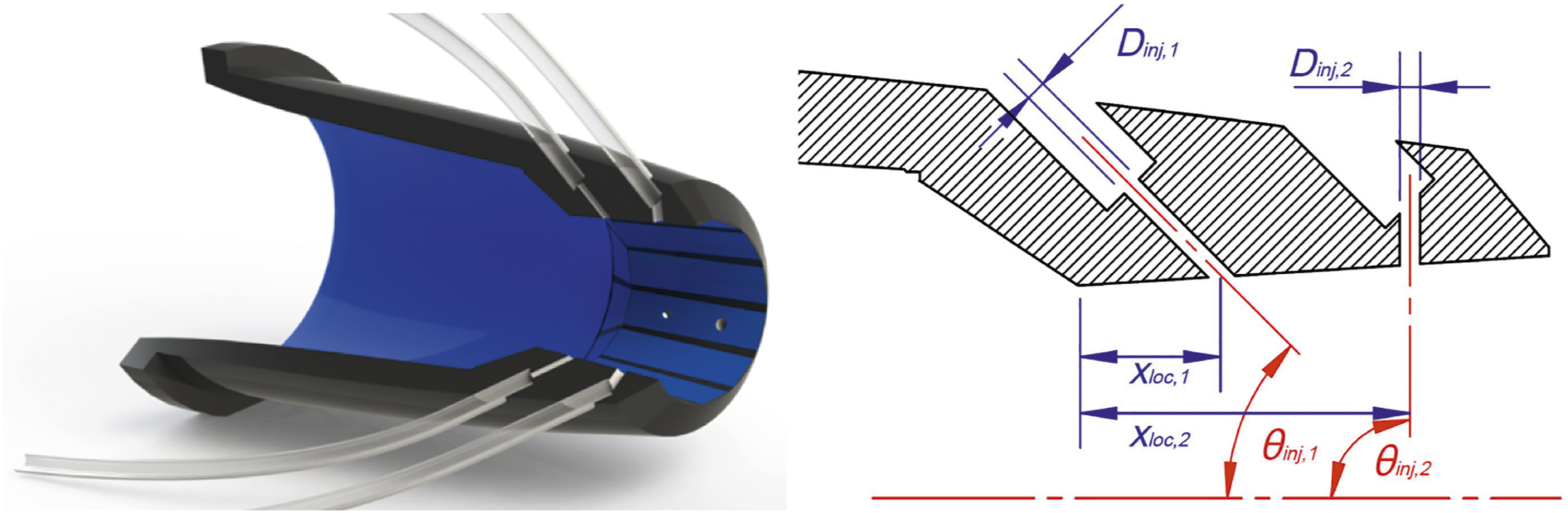
Both the injectors have an exit diameter of D inj = 0.06D e . The upstream injector is inclined at θ inj = 45 o to the jet centerline and is placed at 20% of the distance of the diverging section from the throat to the jet exit. In contrast, the downstream injector introduces air at θ inj = 90 o to the nozzle centerline at 70% of the distance of the diverging section from the throat to the jet exit. Since the individual injectors introduce air at different locations inside the nozzle, for consistency, the injector pressure ratio (IPR) is defined as the ratio of the total inlet injector pressure with respect to the ambient pressure. All the controlled results reported in this investigation use an IPR1 = 1.89 for the upstream injection and an IPR2 = 4.5 for the downstream injector. This is based on previous observations by Prasad and Morris 29 that show that the primary function of the downstream injector in this fluid insert configuration is to provide noise reduction at downstream observer angles, whereas the upstream injector aids primarily in noise reduction in the upstream and sideline directions.
Experimental approach
High speed jet facility description
The experiments described in this investigation were conducted in the Pennsylvania State University’s high-speed jet aeroacoustics facility. A top-down schematic view of the facility is shown in Figure 2. This facility consists of a high-pressure air supply that exhausts into a 5.02 m × 6.04 m × 2.79 m anechoic chamber with a theoretical cutoff frequency of 500 Hz. The downstream section contains an exhaust fan that captures the jet exhaust and minimizes air re-circulation in the anechoic chamber. This single jet facility has been used extensively in several prior jet noise studies.30–32 Other technical details of the facility, including its development, upgrades and flow conditioning can be found in Veltin,
33
Doty
34
and Powers.
31
Top-down view schematic of the Pennsylvania State University high speed jet aeroacoustics facility.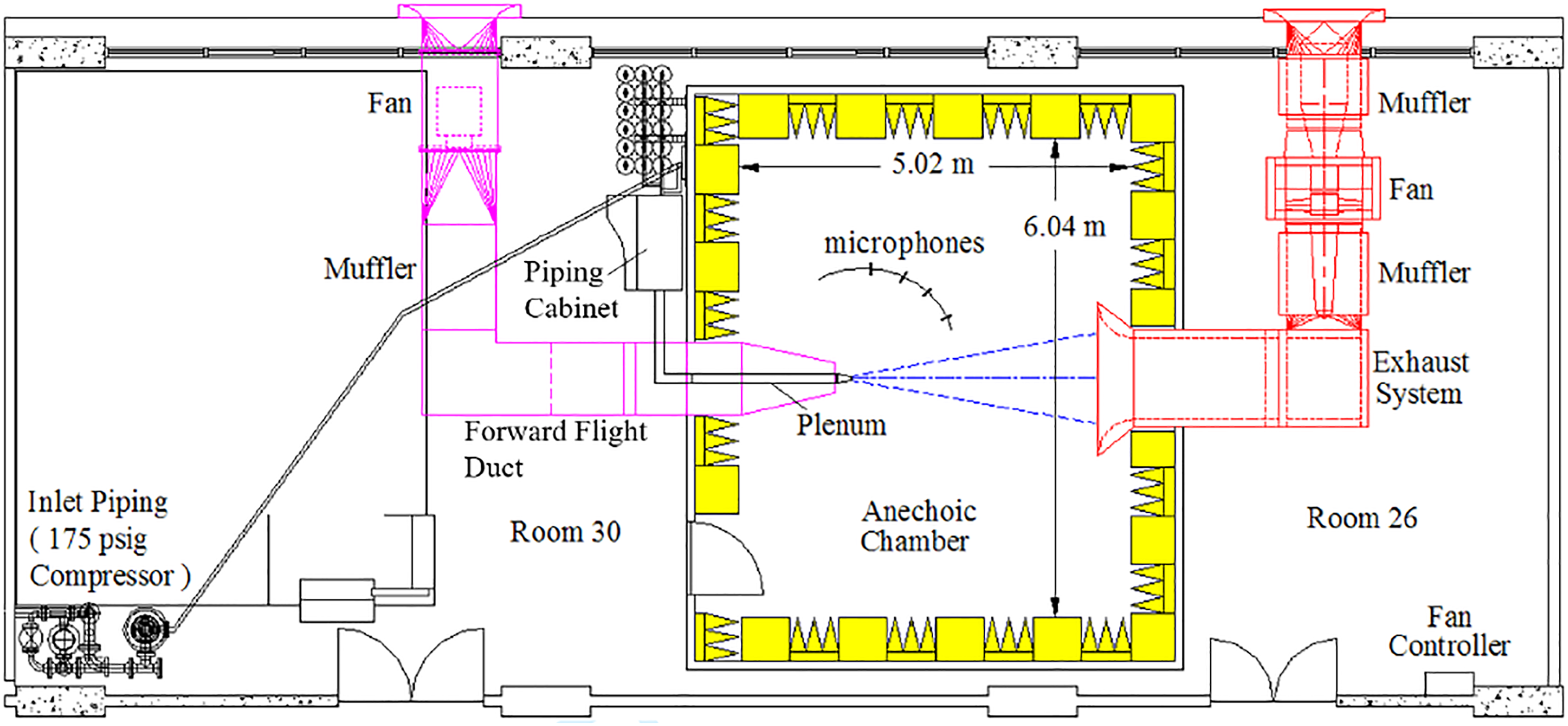
In order to accurately simulate the acoustics of exhaust jets from full-scale aircraft engines, the TTR of the jet must be replicated. The Penn State facility uses helium-air jet mixtures to simulate heated air jets: in the present case, TTR = 3.0. The partial pressures of both helium and air are regulated manually in a piping control cabinet to produce helium-air mixture jets that replicate the lowered density and increased acoustic velocity of heated jets. Three helium cylinders, pressurized to approximately 2100 psi, supply helium into the pressure control cabinet. Accurate mixing of air and helium is achieved via a regulator and gate valve, while the mixture pressure transducer voltage is monitored manually. The mixture’s total pressure is controlled to within 5% of the target value during data acquisition. This methodology, developed by Kinzie 35 and Doty and McLaughlin, 36 has been demonstrated to accurately replicate the noise 37 and velocity profiles 38 of heated air jets. A comparison between experimental data from model-scale heat-simulated jets in the high-speed jet aeroacoustics facility at Penn State and the moderate-scale heated jet noise facility at NASA Glenn Research Center, which show excellent agreement, can be found in McLaughlin et al. 39
Acoustic measurements and data processing
Acoustic measurements are performed with 1/8 in. pressure field, model 40DP, GRAS microphones. These microphones are selected due to their high-frequency response (up to 120 kHz), high peak sound pressure levels (SPLs), and high signal-to-noise ratio. Up to 23 microphones can be mounted on a semi-permanent rotating microphone boom in grazing incidence. The average radial position of the microphones is 85D e , measured from the center of the microphone grid cap to the nozzle exit.
Microphone calibrations are performed with a B&K acoustic calibrator, model 4231. The analog time-domain signals from the microphones are routed through a GRAS model 12AG power module. These signals are amplified and filtered for anti-aliasing, thus enabling their accurate digital conversion in the following data processing. A high-pass filter, set to 500 Hz, is used to remove any undesirable low frequency noise that could contaminate the data. Each microphone signal consists of 409,600 samples acquired at a rate of 300,000 samples per second. The measured data are converted into SPL using Welch’s algorithm. The data is split sequentially into 1024 point segments and a Hanning window function is applied with a 50% overlap between each window. The power spectral density (PSD) is calculated in each window and averaged from all segments. This PSD is then converted to decibels using a reference pressure of 20 µPa.
For each microphone, the SPL is converted to a non-dimensional, lossless value conforming to the ANSI Military Aircraft Measurement Standard established in 2014.
40
Data is corrected for microphone spectral response characteristics based on the manufacturer’s descriptions of each microphone obtained during factory calibration. These include the actuator correction, ΔC
act
(f), and the appropriate free field response, ΔC
ff
(f). The spectra are also corrected for the daily variations in atmospheric quantities during propagation by calculating the atmospheric attenuation (ISO 9613–2:1996) for each microphone using measured ambient pressures, humidities, and temperatures, ΔC
atm
(f), and adding back the sound lost due to the atmospheric attenuation from the jet to the microphone. Finally, the spectra are non-dimensionalized to SPL, SPL per unit Strouhal number, St (= fU
j
/D
e
). Following Kuo et al.
41
the different steps that lead to the SPL per unit St are given by

The microphones are assumed to be in the geometric far-field. Under this assumption, spherical spreading is applied to propagate the acoustic data to a uniform radius of 100D e , measured from the nozzle exit plane.
Noise source imaging
As stated previously, noise source maps are determined from far-field acoustic measurements through a deconvolution of the coherence-based beamformer output. This method was developed and applied to far-field acoustic measurements of an unheated, Mach 0.9 jet by Papamoschou. 15 The present investigation extends the application of this technique to far-field acoustic measurements of heat-simulated, imperfectly expanded jets. A brief summary of the deconvolution-based beamforming method is provided next. Details on the derivation of this method can be found in Papamoschou. 15
The jet noise source is approximated as a linear distribution of spatially incoherent sources, ζ(x, ω), where x denotes the streamwise location and ω is the angular frequency. In the original formulation, this line of sources is typically placed along the jet centerline. However, in order to provide a direct one-to-one comparison with the LES data, we position ζ(x, ω) along the jet shear layer, coinciding at the nozzle lip (x/D
e
= 0, r/D
e
= 0.5) with a 5° spreading angle downstream of the nozzle exit. For a given microphone array, the coherence-based beamforming output, Φ(x, ω), can be defined as


Here G
mn
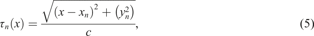
(ω) is denotes the cross-spectral density between the microphones m and n. τ(x) represents the propagation time for a sound wave to travel from any source at position (x, y) along the jet spreading angle to a far-field microphone (x
n
, y
n
) and is calculated using
The coherence-based beamforming output, Φ(x, ω), can be shown to be the convolution of the noise source distribution with the point spread function (PSF) over the streamwise extent of the noise source distribution, L, as follows


The goal of the deconvolution-based beamforming method is to invert equation (6) in order to solve for the coherence-based noise source distribution, ζ(x, ω). For any frequency, the integral in equation (6) can be expressed as the summation over a finite number of discrete sources as follows
Following Papamoschou, 15 we use Richardson-Lucy deconvolution to solve for the discrete source distribution, ζ n . The inversion of equation (8) converges to a residual on the order of 10−5 or less within 75 iterations. The source distribution is calculated over the extent −10 ≤ x/D e ≤ 30 (L = 40D e ), which is larger than the presumed physical extent of the jet noise source. Following the recommendation of Papamoschou, 15 as a compromise between avoiding an unnecessarily coarse spatial resolution at low frequencies and the fine spatial resolution required at higher frequencies, a spatial resolution of Δξ = min (0.01 L, 0.25λ) is selected. Here λ = c/f represents the wavelength of the sound wave.
The positions of the far-field microphones are plotted in Figure 3. The origin is located at the center of the nozzle exit plane. The positions of the microphones on the boom, which were used for far-field acoustic measurements, are plotted as open, blue circles in Figure 3. Deconvolution-based beamforming of the measured far-field data is performed using a more spatially-resolved microphone array, plotted as the red dots in Figure 3. Position of microphones for far-field measurements. The beamforming array is focused on the peak noise emission angle: θ = 135°. Center of nozzle exit plane is located at (x, y) = (0, 0).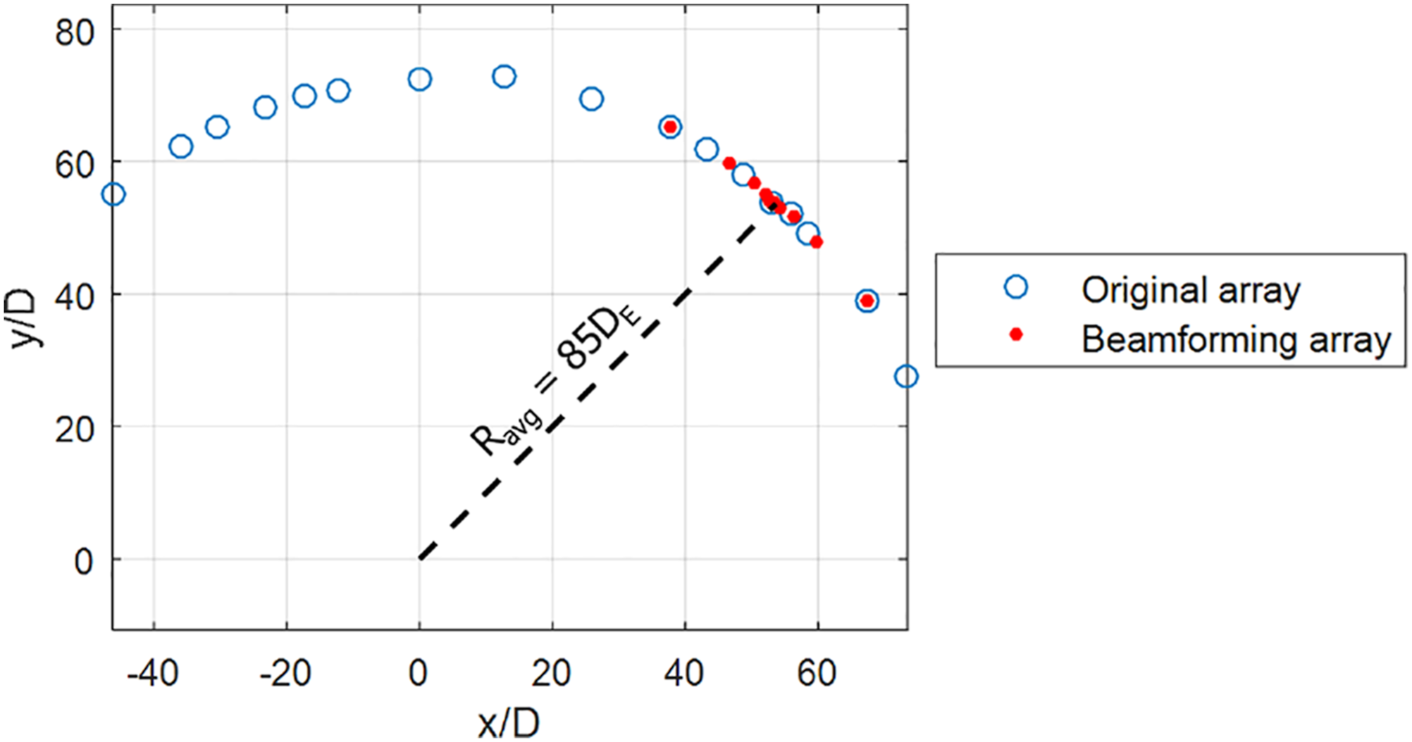
The design of the beamforming microphone array follows the guidance of Papamoschou. 15 All the polar angles are measured from the jet upstream axis. The microphones are concentrated near θ = 135°, the peak noise emission direction. From the θ = 135° microphone, and expanding in either direction to polar angles of 120° and 150°, the microphone spacing is increased logarithmically. Logarithmic spacing is designed to mitigate the effects of spatial aliasing. The angular spacing between the microphones on either side of the θ = 135° microphone is Δθ = 0.4°, with a center-to-center spacing of 12.7 mm. This spacing was chosen as it is approximately half the wavelength of a St = 0.50 sound wave traveling through room-temperature air. This allows a majority of the sources contributing to the high-amplitude turbulent mixing noise to be mapped.
Large eddy simulation database
Formulation and setup
The LES calculations presented in this work are predicated on the previous numerical studies of fluid insert jets conducted by Prasad and Morris18,22,29,42 for moderately larger-scale nozzles than those considered in the present study. The Favre-filtered Navier Stokes equations are solved in their dimensional form using the Wall-Adapting Local-Eddy (WALE) viscosity subgrid scale model 43 on trimmed hexahedral meshes using STAR-CCM+. The mesh distribution is identical to the finest mesh used in Prasad and Morris22,29 and consists of 18.1 M cells for the baseline and 24M cells for the 3FC-2FI nozzle. Prismatic cells with a y+ < 1 are generated at the nozzle walls using the prism layer meshing feature in STAR-CCM+, no wall models are used. The convective fluxes are discretized using a hybrid third-order MUSCL scheme with a normalized variable diagram (NVD) approach 44 for numerical stability near shocks, whereas a second-order central difference scheme is used for the viscous terms. Time integration is performed using a second-order implicit dual time-stepping scheme with 10 sub-iterations.
The streamwise length of the computational domain is 65D e and the radial size varies from 25D e at the inlet to 40D e at the outlet boundaries. All the jets simulated in this work operate at an ambient temperature of 288.15 K and a reference pressure of 101,008 Pa. All external fluid boundaries, except the downstream face, are set as non-reflecting free-stream boundaries based on characteristic variables. The downstream boundary is set as a pressure-outlet boundary. The pressure-outlet boundary condition only requires the specification of pressure and temperature, which are set to ambient values. A sponge zone treatment 45 is also applied to avoid reflections from the outer boundaries. The nozzle inlet is set as a stagnation inlet corresponding to the appropriate NPR and TTR. For the 3FC-2FI jet, the flow through each injector is simulated by specifying the appropriate IPR at the injector inlet. The inside walls of the nozzle are set as adiabatic with no-slip, whereas the outside walls are chosen to be adiabatic slip walls.
Figure 4 shows the instantaneous temperature contours for both the baseline and the 3FC-2FI nozzles at an arbitrary time-step. Instantaneous temperature contours for the baseline (top) and the 3FC-2FI (bottom) jet using LES. The nozzle exit is located at x/D
e
= 0, and the injector ports are located at x/D
e
∼ − 0.26 and x/D
e
∼ − 0.66.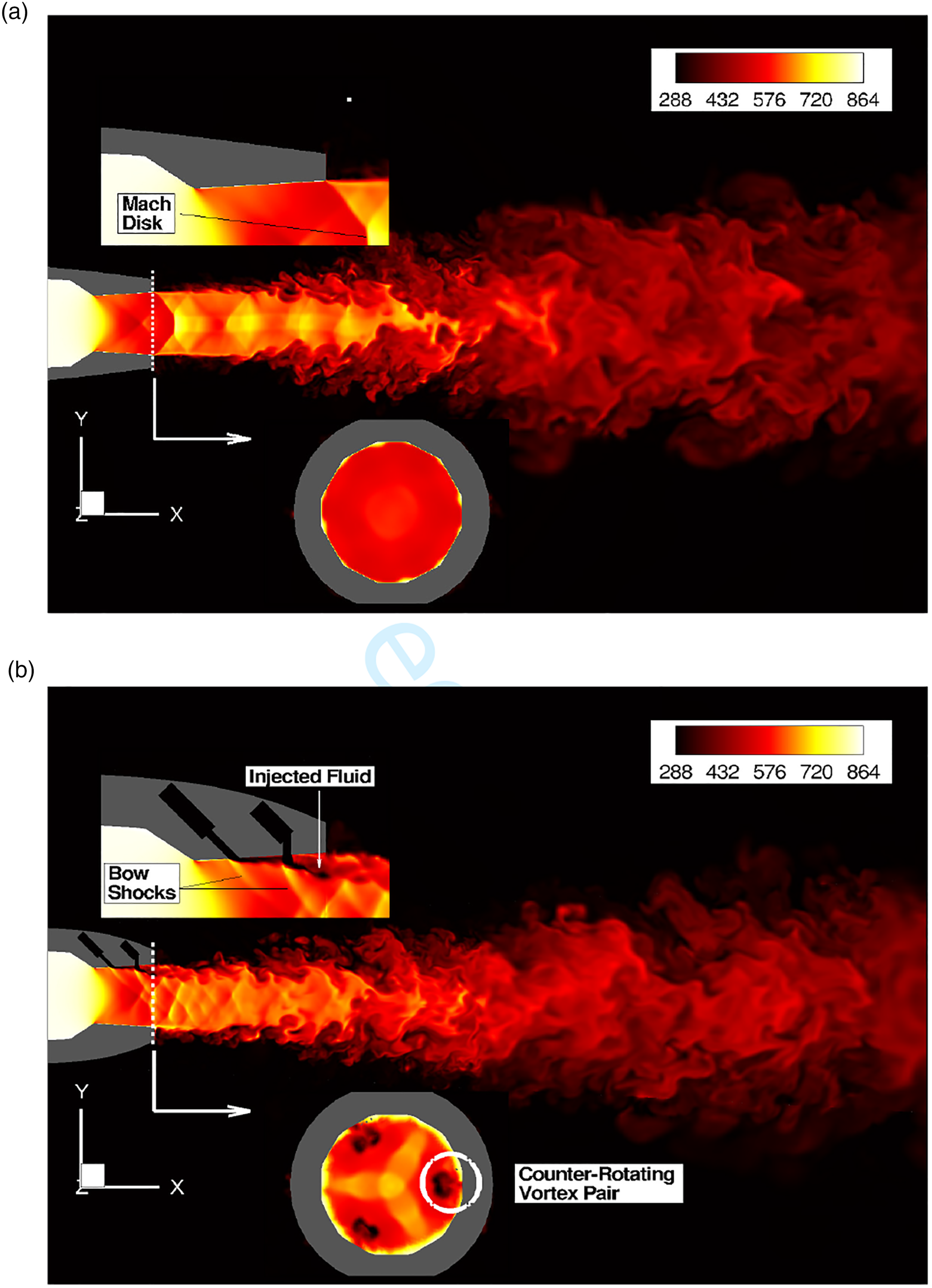
Far-field predictions
The near-field LES results are extrapolated to the far-field using the Ffowcs Williams and Hawkings (FWH) analogy 46 in the time domain with a retarded-time approach. All the far-field observers are located at 100D e from the jet exit. Two approaches are considered in order to obtain the far-field noise signals. In the first approach, the near-field results are calculated directly at 100D e using the FWH analogy, whereas, in the second approach, the experimental procedure for determining the far-field microphone signals is closely replicated. The near-field results are calculated at 85D e using FWH and then propagated to 100D e using spherical spreading.
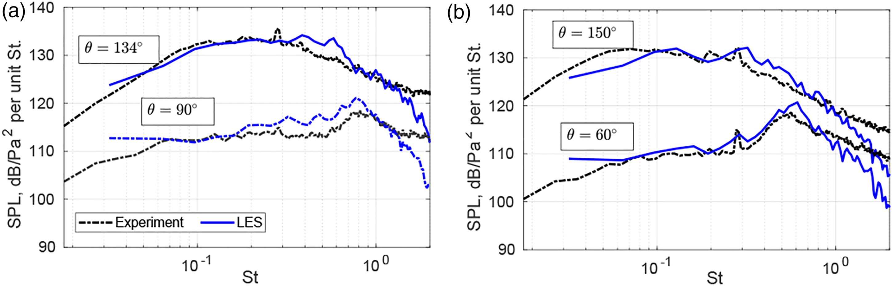
The effect of choosing one method over the other is observed primarily at polar angles where the far-field spectrum changes its shape from a peaked shape to a broadband shape (100° ≤ θ ≤ 125°). This is shown in Figure 5 for the baseline jet at θ = 120°. Directly propagating the LES results to 100D
e
overshoots the LES predictions at 85D
e
that are then extrapolated to 100D
e
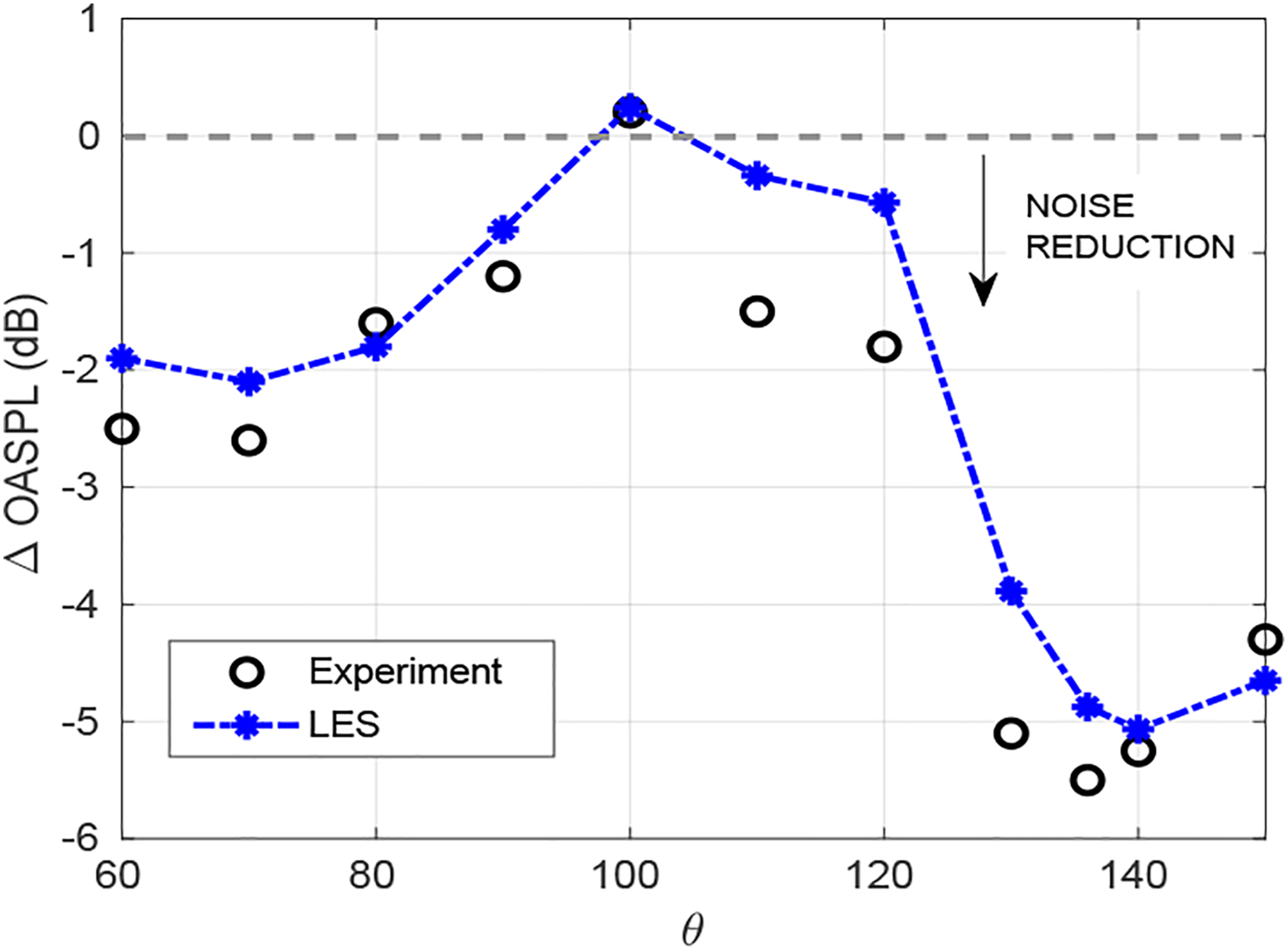
by approximately 2 dB. However, there is a good agreement when the experimental methodology is followed. Effect of the two approaches in extrapolating near-field LES results to the far-field at θ = 120°. Comparison of LES predictions with experimental measurements at different polar angles for the baseline jet. Noise reduction in terms of ΔOASPL for different polar angles with LES and experiments.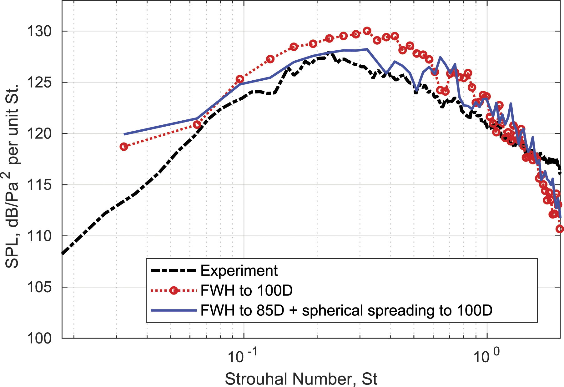
Segregation of radiating and non-radiating components
In order to uncover the mechanisms responsible for the observed noise reductions, the LES flow-field is segregated into its hydrodynamic, acoustic and thermal components using Doak’s MPT.
19
The key step involves a Helmholtz decomposition of the momentum density into its solenoidal and irrotational components, each of which are calculated by manipulating the continuity equation. Following this approach, the momentum density of the flow can be written as


Here primes denote a fluctuation about the mean, which is denoted with an overbar.

The irrotational scalar potential can then be split into its acoustic


Here the subscript ∞ denotes ambient values, C p is the specific heat at constant pressure, and R is the ideal gas constant.
In the solution procedure, the mean solenoidal component
Comparison of noise source imaging with LES
Figure 8 presents the iso-surfaces of the streamwise components of the solenoidal and acoustic components for the two jets at an arbitrarily chosen time-step. Iso-contours of the streamwise component of the hydrodynamic component (top) and the acoustic component (bottom) for the baseline jet (left) and the 3FC-2FI jet (right). Contours of 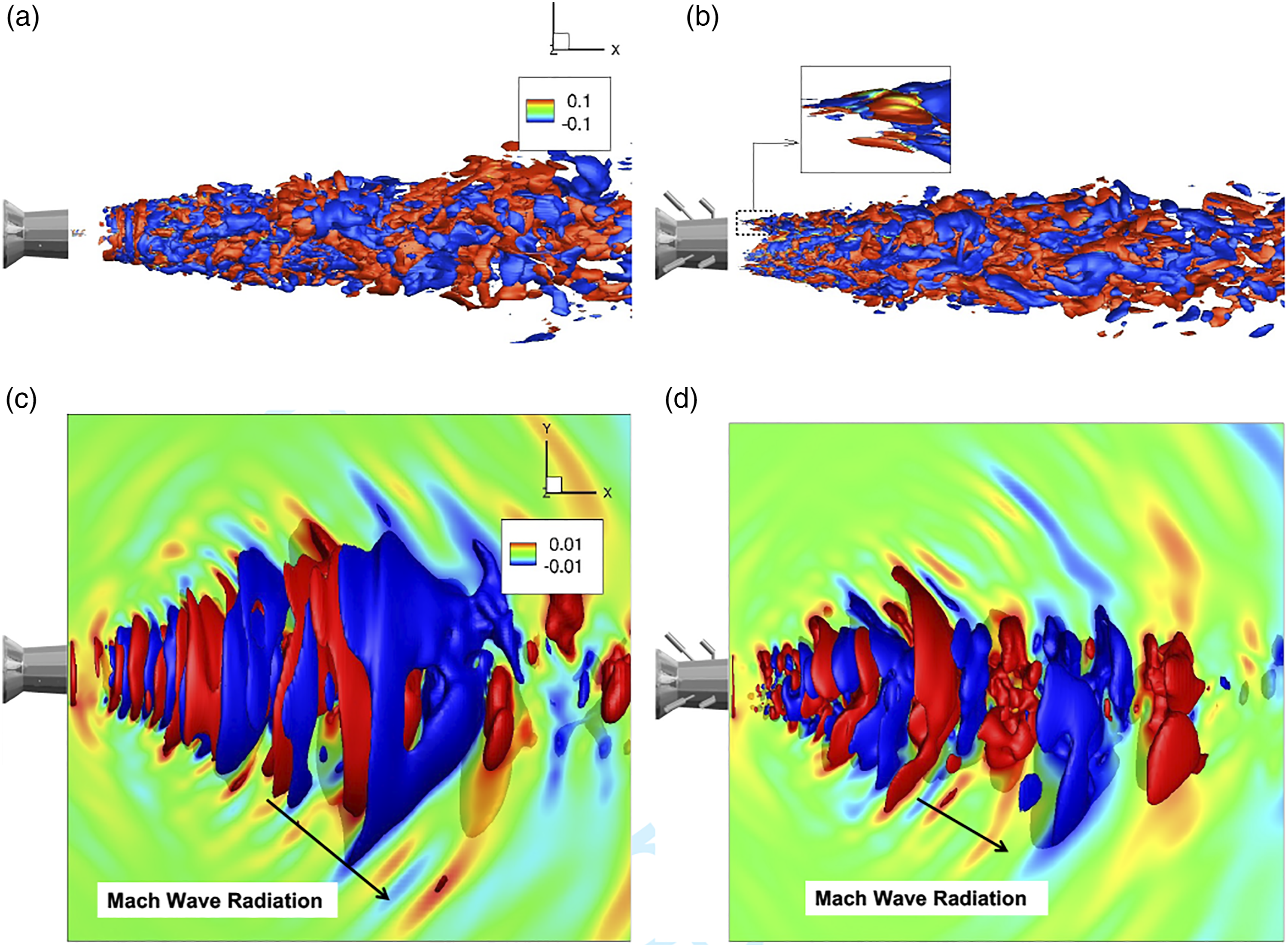
The acoustic component
Although the MPT procedure can separate the hydrodynamic and acoustic components independently, the acoustic component may be considered as an irrotational auditory signature that develops around the turbulent structures represented by the hydrodynamic component;
22
This connection is developed further using SPOD. SPOD is a data-driven technique that decomposes the flow-field into a set of orthogonal modes in the frequency domain that optimally capture the flow’s energy based on a user-defined norm. In the present case, we select a norm consisting of correlated acoustic fluctuations integrated in the peak noise radiation region, as discussed later. The snapshots of hydrodynamic and acoustic components are arranged into a data-matrix

Here
Figure 9 shows the leading Leading 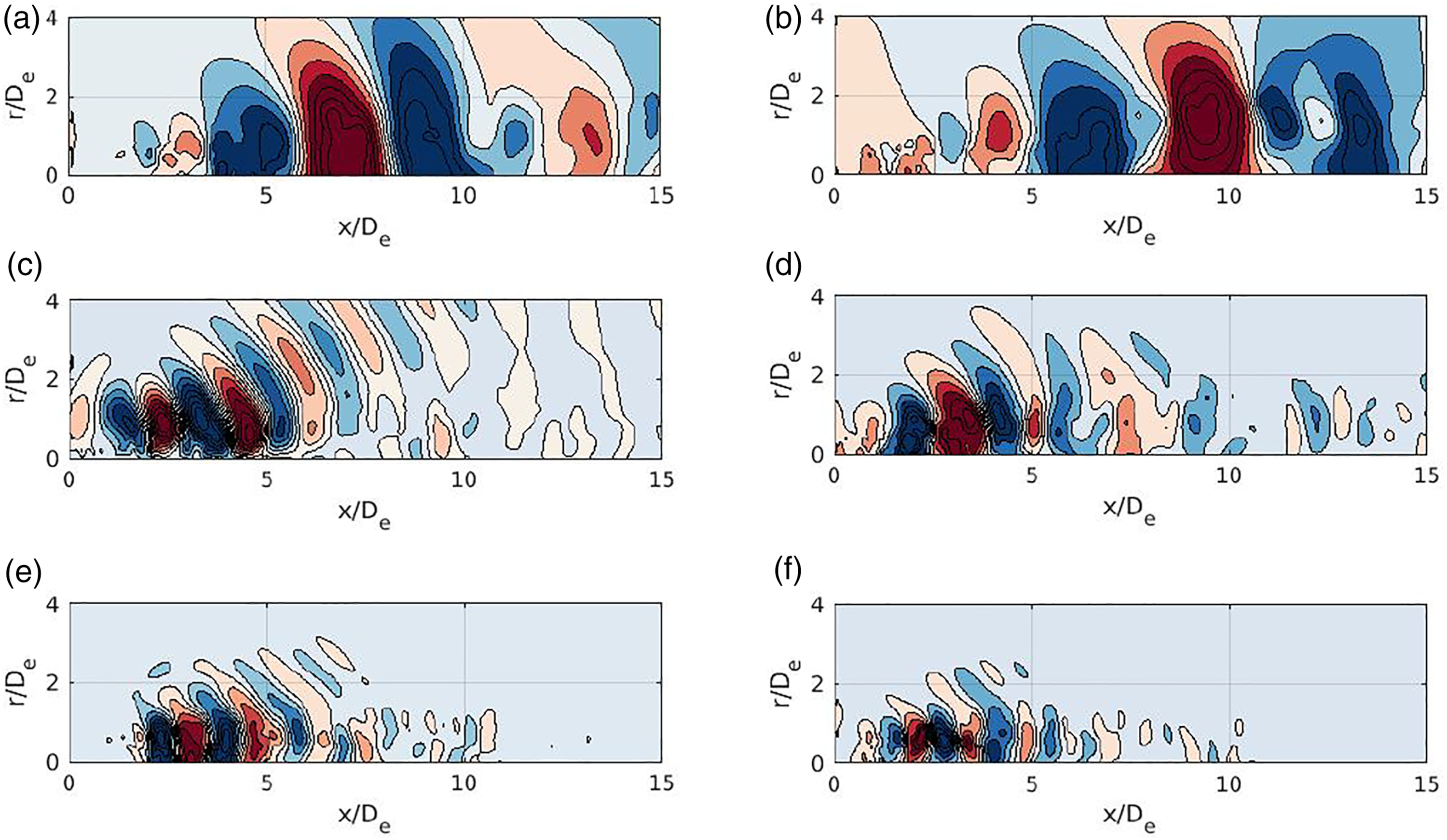
Since these leading Leading 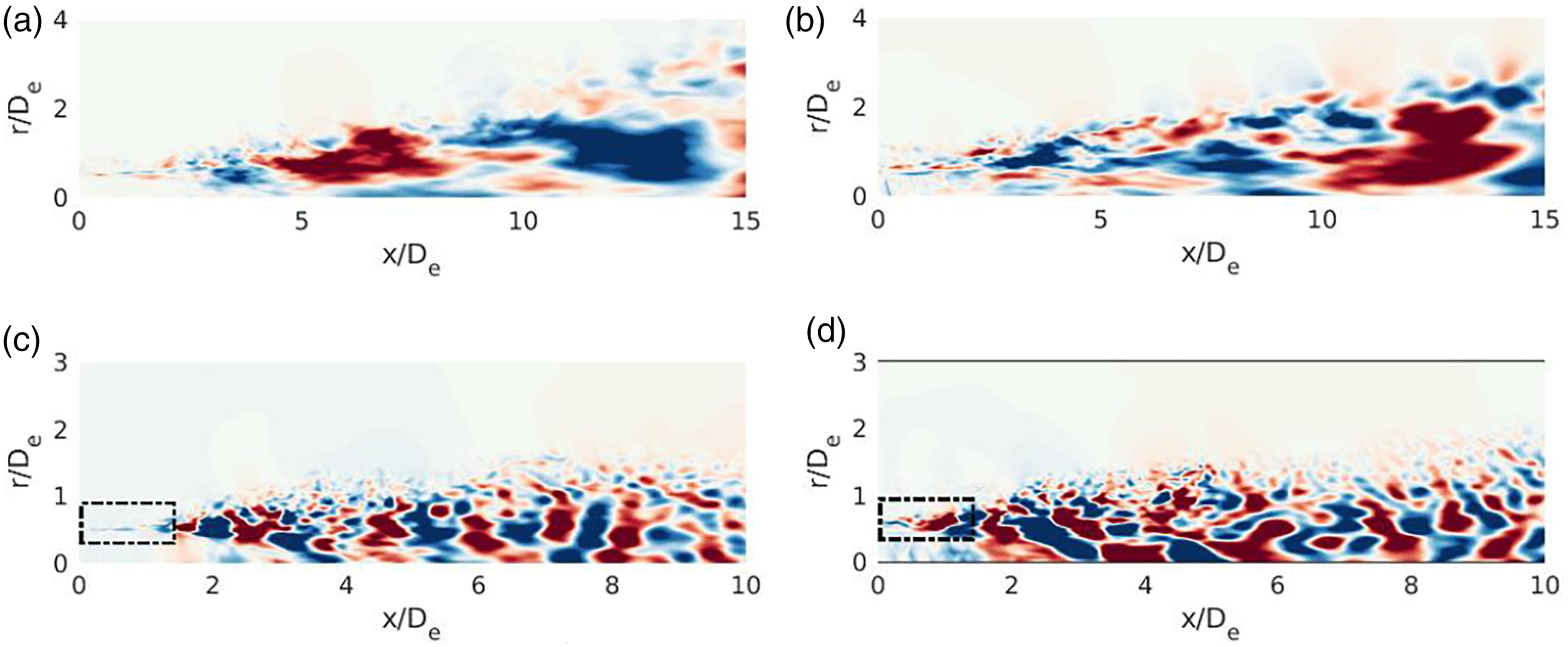
In order to assess the accuracy of the frequency-dependent noise source maps, ζ(x, ω), obtained from the far-field measurements, we treat the acoustic SPOD modes shown in Figure 9 as truth models. Figure 11 shows the noise source distributions at the three St values shown in Figure 9 for the two jets. Noise source maps at the three St values for the baseline (left) and the 3FC-2FI jet (right). The vertical dashed lines indicate the point of peak amplification along the shear layer in the 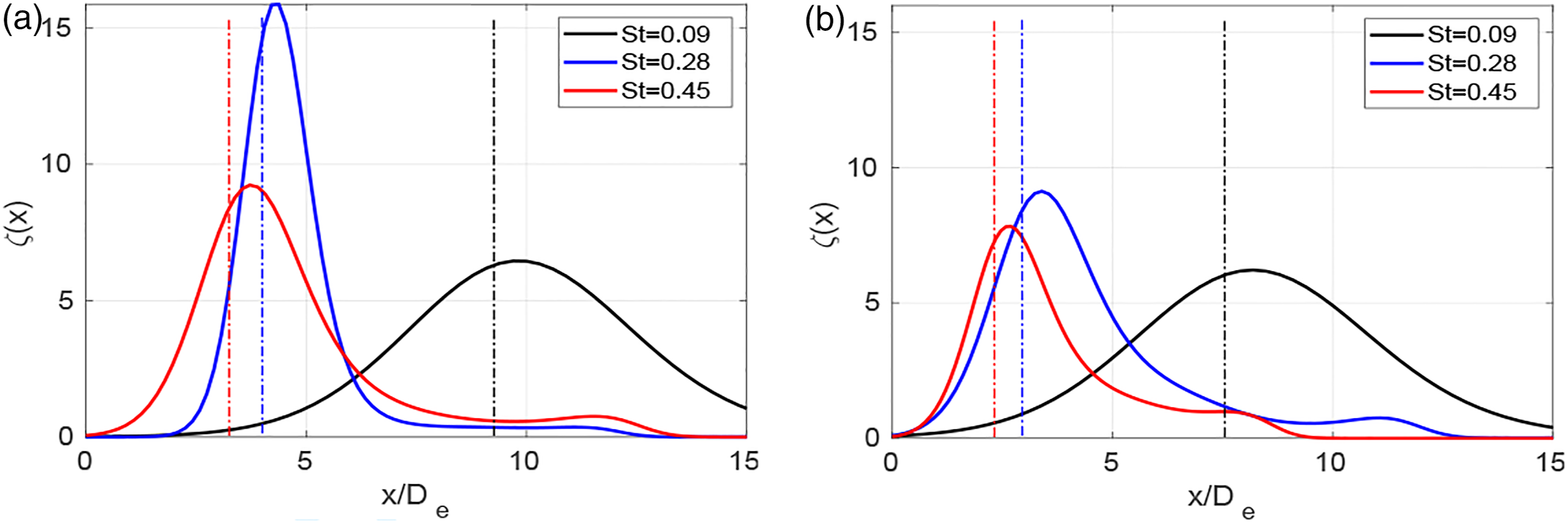
Figure 12 shows the noise source peak locations as a function of frequency, determined from experimental data for both the jets. Comparison of peak noise source location as a function of St value for the baseline and the 3FC-2FI jet obtained from far-field measurements. The horizontal dashed lines correspond to the three St values compared in Figure 11.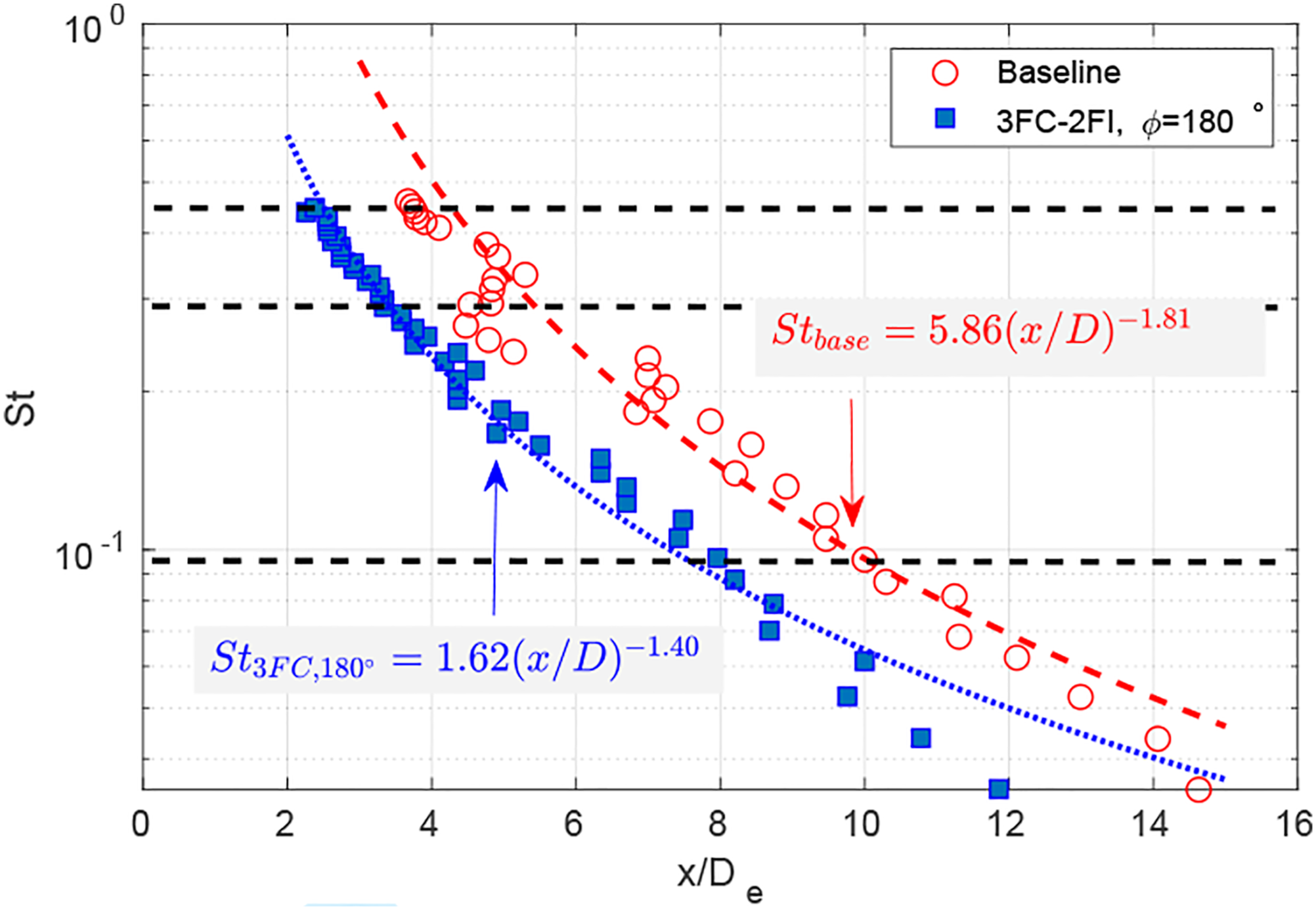
Conclusion
This investigation demonstrates that the effect of fluid inserts on the near acoustic field of an over-expanded supersonic jet can be predicted from the far-field measurements using a deconvolution based beamforming technique. This is achieved by performing two large eddy simulations (LES) corresponding to a baseline and a fluid insert jet to serve as truth models for the experiments. The LES flow-field is decomposed into its hydrodynamic, acoustic and thermal components using Doak’s MPT. When combined with spectral proper orthogonal decomposition (SPOD), the leading SPOD modes of the acoustic component represent a single streamwise structure exhibiting strong Mach wave radiation. These SPOD modes are compared directly with the noise source maps obtained from far-field measurements. It is observed that the use of fluid inserts results in a decrease in the radiation efficiency of the wavepackets which can be attributed to the breaking up of large-scale structures at low frequencies and a modification of the K-H instability at other frequencies. The upstream shift in the peak amplification due to this process is accurately estimated using the noise source maps obtained from far-field measurements. This makes the deconvolution-based beamforming technique a viable candidate for full-scale testing.
Final remarks
It is a privilege for the authors to provide this contribution in honor of Professor John (Shon) E. Ffowcs Williams. Shon was a powerful figure in the development of aeroacoustics beginning with his graduate student days at the University of Southampton. His contributions to the understanding and prediction of the sound generated by high-speed turbulence and by moving bodies remain the foundations for much research more than 50 years after their original publication. The Ffowcs Williams and Hawkings equation and its solution, also used in the present paper, is a key element of computational aeroacoustics prediction methods based on unsteady flow simulations. Professor Ffowcs Williams was a much larger than life character and knew how to enjoy himself. His presence will be greatly missed.
Footnotes
Declaration of conflicting interests
The author(s) declared no potential conflicts of interest with respect to the research, authorship, and/or publication of this article.
Funding
The author(s) disclosed receipt of the following financial support for the research, authorship, and/or publication of this article: This work was funded in part by the Office of Naval Research.