Initial boundary layer state of typical model-scale jet nozzles and its impact on noise

Abstract

A set of 2-inch diameter nozzles is used to investigate the effect of varying exit boundary layer (BL) states on the radiated noise from high-subsonic jets. It is confirmed that nozzles involving turbulent boundary layers are the quietest while others, involving nominally-laminar BLs, are noisier. A turbulent BL is thicker and there is simply an effect of thickness on noise. A thicker BL results in a decrease in the sound pressure spectral amplitudes due to a less vigorous growth of instability waves in the jet’s shear layer. A nominally-laminar BL, besides being thinner, may also involve significantly higher turbulence intensities, much higher than that in a turbulent BL. Such a BL state, referred to as ‘highly disturbed laminar’, results in the largest noise amplitudes especially on the high-frequency side of the spectrum. This transitional state, often encountered with model scale nozzles, involves a ‘Blasius-like’ mean velocity profile but large velocity fluctuation intensities and intermittency. The higher initial turbulence adds to the increase in high-frequency noise. The results leave little doubt that an anomaly noted with subsonic jet noise databases in the literature is due to similar effects of differences in the initial boundary layer state.

Keywords

Jet noise boundary layer initial condition nozzle flow shear layer turbulence

Introduction

The intent of this paper is to revisit the issue of various exit boundary layer (BL) states encountered with model scale nozzles and their impact on the radiated noise. The paper is essentially a summary of the experimental results presented in two NASA Technical Memoranda,^1,2 otherwise unpublished previously. Also, a Large Eddy Simulation (LES) study was conducted at the Naval Research Laboratory (NRL) in Washington, D.C., by Dr Junhui Liu comparing the results with the experimental data of.² The LES results were documented in an NRL report³; highlights of those results are also invoked to advance the understanding of the origin of the various BL states. It should be mentioned here that the author addressed the subject first in 1985,⁴ which was followed by another publication in 2012,⁵ This paper is for the special edition of the International Journal of Aeroacoustics dedicated to the achievements and contributions of Dr Krishan K. Ahuja who, starting from his Master’s thesis work in 1972,⁶ also addressed the issue at hand on various occasions.

While earlier experimental data (e.g., in⁴) demonstrated that a nozzle with a turbulent BL produced less noise relative to its counterpart with a laminar-like BL, a keen interest in the subject arose when Viswanathan⁷ noted an anomaly among subsonic jet noise databases in the literature. He showed that the normalized amplitudes of sound pressure level spectra reported by Tanna⁸ were higher relative to the data at same operating conditions taken in a Boeing facility (Low-speed Aeroacoustic Facility (LSAF),⁷). Figure 1, reproduced from⁷ (also discussed in⁵ and⁹), illustrates the difference between the data of Tanna⁸ and that from LSAF.⁷ The Tanna data are consistently larger in amplitude on the high-frequency end. This was a serious issue since these datasets have been the basis for validation of jet noise prediction codes.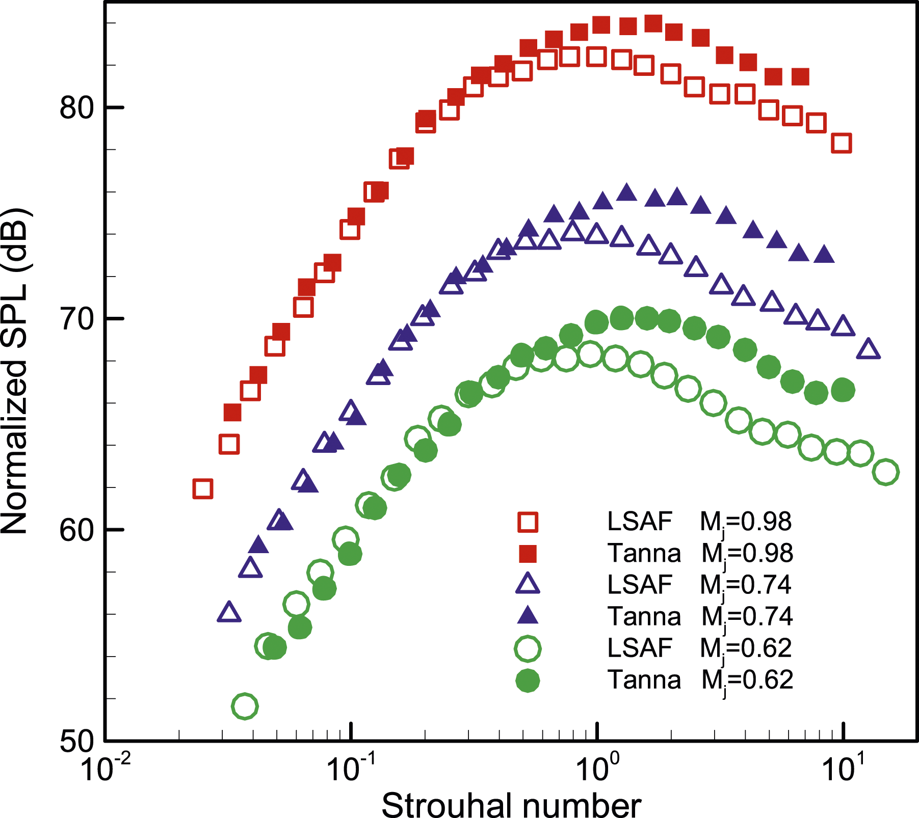

Figure 1.

Discrepancy in sound pressure level spectra (one-third-octave format) between measurements of Tanna⁸ and Viswanathan⁷; θ = 90°. Graph is copied from Ref. [7].

The contrast between data from ‘University-type’ facilities^8,10,11 and ‘Industrial-type’ facilities^7,12,13 was further identified and discussed by Harper-Bourne.¹⁴ Viswanathan⁷ had speculated that a higher rig noise in the Tanna facility must have caused the higher noise. Harper-Bourne, however, recalled that extensive internal silencing was performed in that facility and rigorous tests were conducted to validate its quality. Recently, Karon and Ahuja,⁹ conducted further tests in the Tanna facility (now in their custody) to rule out rig noise, as discussed further in the following. With regards to the University versus Industrial type facilities, Harper-Bourne noted that the University types, exhibiting higher noise, had large contraction ratios. Contraction ratio could affect the flow quality and the exit BL state, but these parameters were not measured with the cited datasets and the real reason for the noise difference remained unexplained.

Following the astute observation of spectral amplitude difference by Viswanathan,⁷ Viswanathan and Clark¹⁵ conducted another important investigation. They studied the effect of exit BL state on noise using three nozzles of same diameter (2”) but having different upstream flow paths: a ‘Conic’, a ‘Cubic’ and an ‘ASME’ contour. The Conic had a slow convergence up to the exit whereas the other two had an abrupt convergence from a large diameter to the exit diameter. The ASME design, with a quarter-ellipse-shaped contraction to produce uniform flow with a thin BL, is used widely for flow calibration nozzles; it is discussed more in the next section. The main difference between the Cubic and the ASME nozzle was a 1D long cylindrical section at the end of the latter but none with the former. The idea with the Cubic was to produce a very thin BL. They used computational Fluid Dynamics (CFD) as well as measurements of nozzle discharge coefficient to infer that the Cubic indeed had the thinnest BL (δ = 0.04”), the Conic had the thickest (δ = 0.20”), while the ASME had an intermediate thickness (δ = 0.12”); δ is based on the location of 0.99U_J point, U_J being the jet velocity. Based on re-laminarization criteria (discussed in the next section) they inferred that the BL for the Conic nozzle must be turbulent while that for the Cubic was likely laminar. Surprisingly, these two, with the thickest and the thinnest BL, produced almost identical far field noise spectra. Based on this evidence, they thought that the amplitude difference in Figure 1 could not be due to a difference in BL thickness and must be due to internal rig noise in.⁸ However, as stated earlier this inference is likely incorrect.

Curiously, Viswanathan and Clark¹⁵ observed that the ASME nozzle, having the intermediate BL thickness, had larger high-frequency spectral amplitudes relative to the Conic case, bearing a striking similarity with the difference noted in Figure 1. (We note here that the Cubic case actually has slightly higher noise relative to the Conic case but the noise for the ASME case is much larger.) They reasoned that the cylindrical section of the ASME nozzle, “…allowed the laminar BL to have an opportunity to grow and reach a state of transition at the nozzle exit”. Such a state might have amplified disturbances in the external shear layer leading to the higher noise. Note that they did not have direct BL measurements. They underscored the importance of especially turbulence measurement and said that “only measurements of turbulence levels at the nozzle exit and in the immediate downstream region” would settle the issues.

Probable causes for the anomaly in Figure 1 were explored in.⁵ Among other parameters, turbulence intensity in the jet core was varied over a range of 0.15% – 5% (in terms of r.m.s. amplitude as percent of U_J) by using turbulence generating grids upstream of the nozzle. Amplitudes of far-field noise spectra were found to increase with increasing core turbulence. This observation ruled out core turbulence as the source of the anomaly. The University-type facilities had large contraction ratios as well as flow conditioning units so that the turbulence at the jet exit was minimized, whereas those were the ones that yielded higher noise.

Taking a cue from,¹⁵ the effect of nozzle interior shape was also examined in.⁵ Two 1-inch diameter nozzles were fabricated mimicking the Conic and the ASME shapes and a difference in the noise levels, as reported in,¹⁵ was readily confirmed. The noise levels for the ASME nozzle were significantly larger. The earlier work of⁴ strongly suggested that a difference in the exit BL state might be the cause for the difference. This was indeed confirmed with BL measurements. It was shown that the ASME nozzle involved a ‘nominally-laminar’ initial boundary layer with a large turbulence intensity. This contrasted the Conic case that had a turbulent boundary layer with much lower turbulence intensity. (The term ‘turbulence intensity’ is used for simplicity even though in the laminar-like case the BL is transitional and involves large intermittency.)

Here, a discussion of the initial boundary layer state is in order. When the BL is thin relative to the nozzle diameter, the velocity profile along a radial line should be similar to that over a flat plate.¹⁶ A fully laminar state is characterized by a Blasius mean velocity profile with a shape factor of about 2.59. The turbulence intensities are small and about the same as that in the core of the jet. A fully turbulent state, on the other hand, is characterized by a slow and prolonged decay of mean velocity as the wall is approached. This is followed by a sharp decrease in the mean velocity near the wall, with near-wall turbulence intensity peaking to 10%–12% of the jet velocity as in a flat plate BL. (Actually, peak turbulence is often much lower in the turbulent BL of convergent nozzles, as discussed further with the data). In practice, with laboratory jets, a fully laminar state is seldom encountered. Quite often the BL is found to be in a disturbed laminar-like state. The mean velocity conforms to the Blasius profile with a relatively large shape-factor, but the turbulence intensities are high. This is broadly referred to as a ‘nominally-laminar’ state. A test for distinction between nominally-laminar and turbulent states may come from a plot of boundary-layer thickness versus Reynolds number. For a nominally-laminar state, the thickness would decrease following a 1/Re_D^1/2 proportionality with increasing velocity. Transition to a turbulent state would be marked by a jump in the thickness, followed by only a marginal decrease in thickness with roughly a 1/Re_D^1/7 proportionality.

The nominally-laminar state is a transitional state and there may be different levels as affected by the history of the upstream flow path, pressure gradients and background disturbances. The turbulence intensity is sometimes quite high, much higher than that in a turbulent BL. This has been referred to as a ‘highly disturbed laminar’ state which is a common occurrence with laboratory nozzles. So, in the following we will differentiate the BL state from fully laminar to nominally-laminar to turbulent categories, the highly disturbed laminar state being a subclass of the nominally-laminar state. (By the same token there could be a ‘nominally-turbulent’ state, however, for the model jets considered in this study different levels of turbulent state are difficult to differentiate; once transition takes place the velocity profiles appear similar although there could be some differences in the shape-factor and peak turbulence level.) Note that the term ‘laminar-like’ is used synonymously for the nominally-laminar state.

A review of past work on the subject, far from being exhaustive, is given here. Several earlier studies addressed the effect of nozzle exit BL condition on the jet flow field [e.g.,^17–23] as well as radiated noise.^24–28 While some of the flow field results are invoked in later discussions, the focus in this paper is on the far field noise. Salient features of the results from,^24–26 discussed in detail in,⁴ are repeated. Mollo-Christensen²⁴ presented data with and without BL tripping (at Re_D = 10^6); the noise spectral amplitudes were found to be somewhat lower for the tripped case, as also observed in.⁴ Maestrello and McDaid²⁵ compared data from a short versus a long nozzle and noted that the long one had lower spectral amplitudes. Apparently the short one had a laminar BL while the long one had a thicker, turbulent BL. Grosche,²⁶ using an elliptic mirror technique, showed that BL tripping largely reduced sound source intensity near the nozzle. Bridges and Hussain²⁷ demonstrated noise radiation from vortex pairing activity for an initially laminar BL. This was also evident in⁴; the noise due to vortex pairings got suppressed when the BL was tripped. It is worth mentioning here that Crighton²⁸ noted a difference in jet response to external perturbations across a Re_D range that is likely tied to differences in the jet’s initial BL state.

It is needless to mention that apart from^7,8,10–13 many other experimental studies contributed to jet noise databases and helped develop and validate theoretical predictions for jet noise. These include K. K. Ahuja’s work from early 1970s, e.g.,.²⁹ C. J. Moore³⁰ noted small differences between his and the data of²⁹ underscoring the fact that jet noise could be susceptible to differences in facility and nozzle geometries. Reference [30] is a rare earlier work that reported turbulence data at the nozzle exit. The exit turbulence intensity profiles were measured for three different configurations including one with a BL trip. However, the overall jet flow field downstream appeared similar, and far field noise difference was not reported and apparently assumed to remain unaffected.

Relatively recently, a large number of numerical as well as a few experimental studies have been conducted on the initial BL effect as well as the effect of upstream conditions on flow and noise.^31–47 Most of the studies on initial BL effect were comprehensive also analyzing the flow field evolution and its stability characteristics but here we focus on the far field noise vis-à-vis the exit BL state and thickness.

Uzun and Hussaini³¹ studied high-frequency noise generation for an initially transitional BL and noted noise radiation at vortex pairing frequencies yielding distinct spectral peaks. These results conformed to experimental observations, e.g., in.^4,27 Bogey, Barre and Bailly³² studied a jet from a straight pipe with constant BL thickness but with largely different turbulence levels. They found that the jet with lower turbulence produced more noise apparently because of vortex pairing activity. Bogey and Bailly³³ also studied jets with laminar exit condition where the momentum thickness and turbulence intensity were varied. Far field noise spectral shapes with varying initial momentum thickness were found to be remarkably similar to those reported in.⁴ Adding random disturbances in the upstream pipe flow, apparently mimicking BL tripping, suppressed vortex pairings and hence noise as in the cited experiment. This result was further confirmed by simulating jets with tripped BL in.^34,35

Bogey, Marsden and Bailly³⁶ investigated jets issuing from a pipe where the Reynolds number was varied (by varying D) from 2 × 10^4 to 2 × 10^5. At higher Re_D lower noise was noted and this was ascribed to variation of other parameters such as exit BL condition rather than Re_D per se. Several studies indicated that simply a thinner BL (laminar or turbulent) may produce higher turbulence in the ensuing flow and a higher resultant noise. Bogey and Marsden³⁷ varied the BL thickness from 0.045D to 0.21D, in one case keeping the Reynolds number based on nozzle diameter (Re_D) fixed and in another case keeping the Reynolds number based on BL momentum thickness (Re_δ2) fixed. In all cases the peak turbulence intensity was held constant at 9% and the jet Mach number was 0.9. A thicker BL produced less energetic coherent structures downstream yielding lower OASPL at all angles. A thicker BL reduced noise regardless of the BL state.

Bogey and Marsden³⁸ later studied jets issuing from pipe flows but simulating the difference of the ASME and Conic nozzle BL states.^5,15 Unlike in the experiments, however, far field noise was found to be similar. They concluded, “…link between the noise differences and the jet initial conditions using the two nozzles might not be as simple as was first thought, and that other parameters, associated for instance with the nozzle geometry such as the presence of pressure gradients, might also play an important role.” In yet another LES study, Bogey and Sabatini³⁹ kept the momentum thickness and peak turbulence intensity constants (0.0014D and 0.06U_J, respectively) but varied the BL shape factor from 2.55 to 1.52. In the laminar case (shape factor 2.55), the jet flow development was faster, leading to a shorter potential core, higher rate of centerline velocity decay and higher noise. Linear stability analysis supported those results. Bogey⁴⁰ further simulated the ASME versus Conic nozzle behavior by performing LES with laminar versus turbulent BL profiles but with imposition of higher turbulence in the laminar case. The laminar case did radiate higher noise as seen in the experiments.

Brès et al.⁴¹ simulated subsonic jets also from a pipe nozzle at Re_D of 10^6. Use of synthetic turbulence produced a turbulent exit BL matching closely with the data from a companion experiment in their study. LES results on far field sound pressure spectra matched with the experiment to within 0.5 dB. In contrast, a laminar exit BL produced high spectral amplitudes on the high-frequency end as seen in prior experiments. The laminar case, however, had a lower turbulence intensity compared to the turbulent cases, contrary to the nominally laminar BL in prior experiments.⁵ The noise increase was a thickness effect; the thinner laminar BL produced more noise due to differences in the growth rates of the (Kelvin-Helmholtz) instability waves in the near-nozzle region. With the thinner BL the overall growth was more vigorous leading to higher turbulence and noise. The conclusion applied to various azimuthal modes of the instability waves, and they further noted that the noise amplitude difference was more pronounced on the sideline relative to that seen in the peak noise radiation direction (downstream). A similar LES study, with accompanying experiment, was carried out more recently.⁴² An emphasis was to speed up the solution turn around time. The numerical results validated well against flow and noise data from the Institute of Sound and Vibration Research (ISVR) Laboratory of University of Southampton, UK.

On the experimental side, BL measurements were performed by Karon and Ahuja.^9,43–45 These experiments were conducted in the same facility where the Tanna data,⁸ exhibiting higher noise in Figure 1, were acquired. Authors first went through measurements to disprove that rig noise was a factor. They demonstrated this by measuring noise with nozzles of different diameters and checking that the intensity variation followed expected theoretical trends as well as by measuring noise with and without a muffler in the upstream duct.^9,43 The muffler did not make a difference in the noise, thus, demonstrated the absence of significant rig noise. They then conducted noise measurements for ‘ASME’ and ‘Conic’ shapes (as in¹⁵ and⁵). Somewhat surprisingly, the two shapes with 2” exit diameters did not produce a difference in the noise; the BL velocity profiles were similar as well. However, with smaller diameters (D = 1.5”), a pronounced difference did occur for the two internal shapes. For the latter cases, BL velocity profile measurements showed that the Conic and ASME nozzles had a large difference in the shape factor commensurate with turbulent and laminar states, respectively. The authors noted that the lack of difference exhibited by the larger pair of nozzles was possibly linked to differences in the upstream path; the 2” and 1.5” conical nozzles were not geometrically similar. They also discussed Dr Ahuja’s earlier study⁶ where he used pipe extensions to thicken the BL and found that a thicker BL produced lesser noise. They provided an analysis to demonstrate that the spectral levels increased systematically with increasing shape factor. However, the effect of initial turbulence levels went unaddressed since their BL profiles were obtained by stagnation pressure measurement with Pitot probes.

Another elegant experiment was performed by Fontaine et al.⁴⁶ using particle image velocimetry (PIV). They explored the flow field very near the nozzle exit together with far field noise measurement. They used pipe extensions of three lengths, L/D = 2.37, 10.9 and 19. In addition, they used a smaller diameter (0.76”) nozzle with internal contour similar to the Conic case and a larger diameter nozzle with an ‘ASME-like’ interior (the contracting section of the latter nozzle had a polynomial contour, further discussed in the next section, reducing from 3.98” to a 1.36” diameter cylindrical section at the end). For the pipe cases, progressively thicker BLs were measured with longer extensions. From a criterion of momentum thickness variation with Re_D they inferred that these boundary layers were turbulent. The peak turbulence intensity for the three cases were comparable and in the range of 12% – 14.5%. They inferred that, “one obvious effect of thicker nozzle boundary layers is to reduce noise”, although this could be confusing from the overall trends of their noise data. (Their Figure 15 shows that both the long pipe with the thickest BL and the small D nozzle with the thinnest BL produced comparable and lowest noise levels among the five cases. The ASME-like nozzle had an intermediate BL thickness but produced the highest noise level. Unfortunately, they did not provide turbulence data for the two nozzle cases that might have shed further light). Their inference pertains to the high-frequency end of the spectra and they made an important observation that when the far field noise data were scaled by the initial momentum thickness, the spectra collapsed on the high-frequency end. A set of data from the present investigation will be examined in this format.

Thus, from the review of the studies^31–46 as well as¹⁵ a somewhat confused picture emerges as to the effect of the initial BL on radiated noise. Several questions come up. Is the effect seen in the far field noise simply a BL thickness effect? For a specific Re_D and geometry, will a thin BL always produce higher far field noise? What is the relative impact of initial turbulence on noise? Many of the reviewed studies (simulation and experiment) were conducted with variable length pipe flows; does this make a difference relative to jets issuing from convergent nozzles? In,⁵ 1” diameter nozzles were used; how does nozzle size and Reynolds number affect the BL state? Also, the noise data in⁵ were obtained in a semi-anechoic environment; an accurate set of noise data with the nozzles being examined was highly desirable. This led to a continuation of the experiments. A set of 2-inch diameter nozzles were used, including a Conic, four ‘ASME’ cases and another one (‘SMC’), described further in the following section. Exit boundary layer data and far field noise data were acquired. The results are discussed with an eye to answering some of the questions posed.

The experimental hardware and procedure are discussed take out next. In the Results section, data for the Conic and ASME-type nozzles are presented first. The BL data are discussed here followed by the noise data. In the following subsection, data for the SMC case are discussed briefly, followed by key LES results of.³ Digital files of the experimental data as well as the coordinates of all nozzles can be found in¹ and.²

Experimental procedure

All flow-field data are gathered in the ‘CW17’ open jet facility at NASA GRC.⁵ A picture is shown in Figure 2(a). Compressed air passes through a 30″ diameter plenum and through the nozzle to discharge into the quiescent ambient of the test chamber. All nozzles are convergent and have a 2” exit diameter; all dimensions are given in inches. An ASME nozzle is shown in Figure 2(b) while Figure 2(c) shows the Conic nozzle. All ASME nozzles fit to the adapter seen in Figsure 2(a) and (b), the Conic nozzle is attached to a different adapter. Yet another adapter is used to attach the SMC nozzle seen in Figure 2(d). Figure 2(e) shows the SMC nozzle together with a pipe extension which is referred to as SMC+. The pipe is 12” long with 2.25” internal diameter. Figure 2(f) shows a closeup view of a hot-wire probe about 0.030” downstream of a nozzle lip for BL measurements.

Figure 2.

Experimental arrangement. (a) Open jet facility, (b) ASME design nozzle, (c) Conic nozzle, (d) SMC nozzle, (e) SMC nozzle with a 12” long pipe upstream, (f) hot-wire setup for exit boundary layer measurement.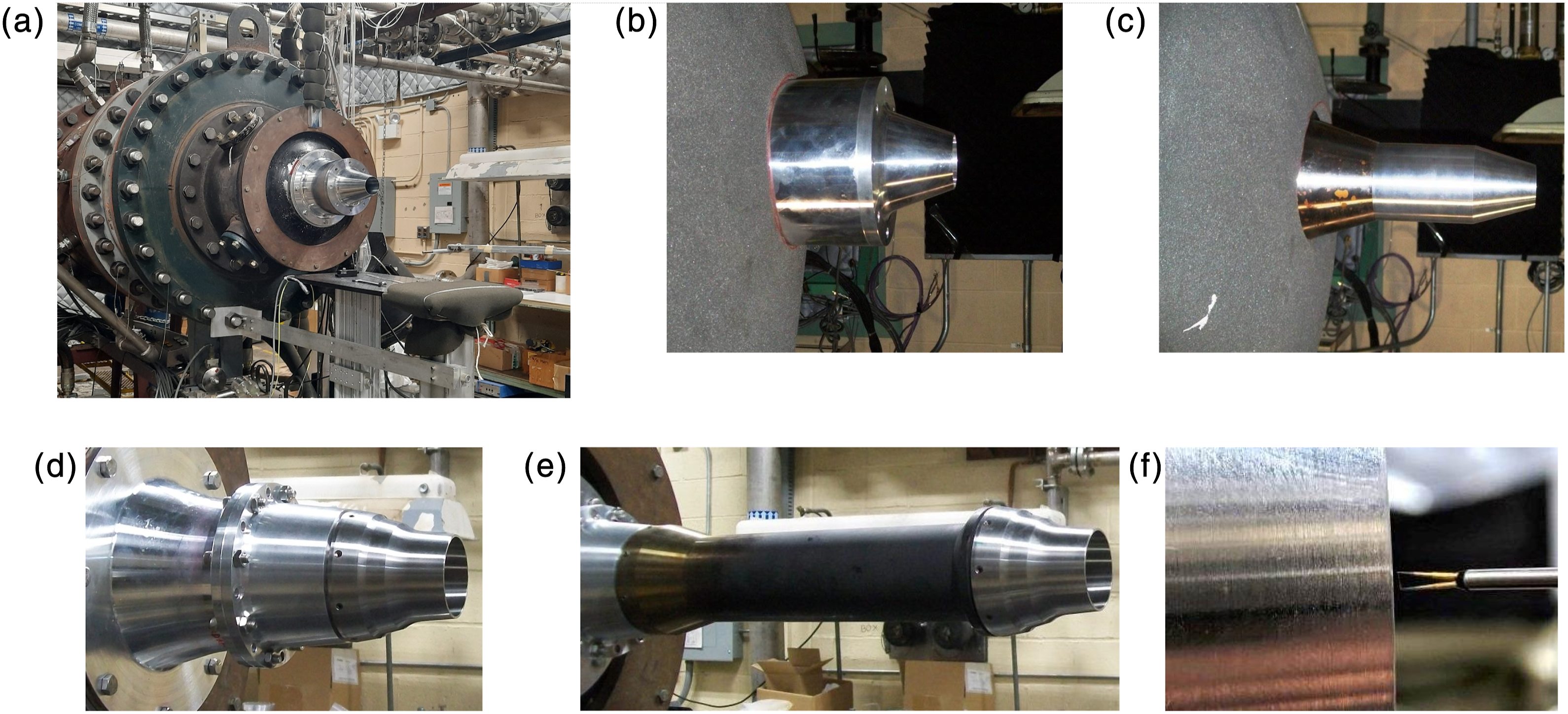

The internal contours of the Conic and ASME design cases are shown in Figure 3. The upstream section of all nozzles, which attaches to the plenum chamber, starts with a diameter of 5.16″ and an initial slope (dr/dx) of −0.32. The Conic case contracts down to a 2.558″ diameter cylindrical section (blue line in Figure 3(a)), at the end of which is the conical section (light blue line). The conical section contracts down to a 2″ diameter exit over a length of 3.32″; thus, the half-angle of convergence is 4.8°. (It is noted here that having a small convergence at the end of the nozzle is a common practice in the industry. The reason for the practice is not clear to the author's knowledge. Perhaps, it is done with the expectation that the BL would be laminar and thinner and hence improve thrust. However, as discussed in the following, a small convergence actually sustains the turbulent BL state.)

Figure 3.

Nozzle contours. (a) Conic, (b) ASME design (dotted line explained in text), (c) convergent section of four ASME cases; ordinate pertains to the Short case and others are staggered by 0.5”. Black dots in (c) denote locations where ‘acceleration parameter’ is equal to 2 (see text). (Four ASME cases, Figure 3(c), are referred to as ‘Long’, ‘Dsgn’, ‘Sh-e’ and ‘Shrt’).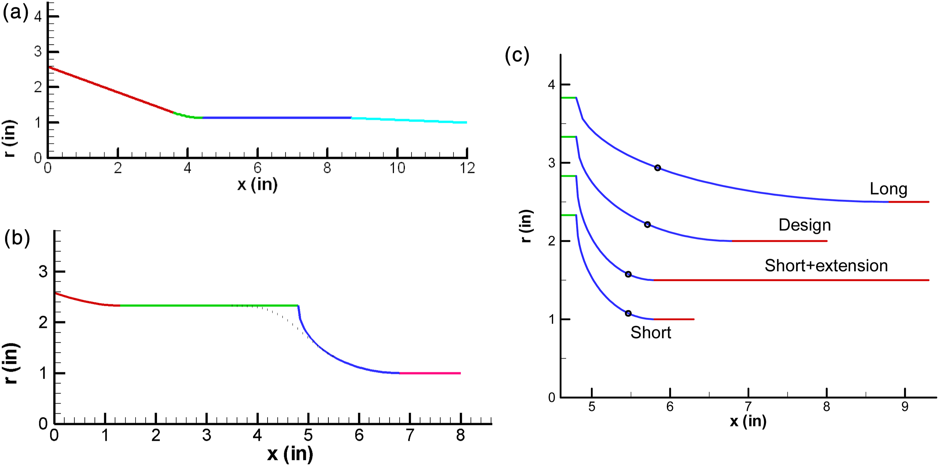

The interior of each ASME case has a common 4.66″ diameter cylindrical section of length 3.5″ (green line in Figure 3(b)). At its end, end-pieces of various designs are attached. The combination of blue and red lines in Figure 3(b) represents the end-piece for the ‘ASME design’ nozzle. The convergence takes place over the length of the quarter-elliptical blue line while the red line at the end is a cylindrical section. (Often a model scale nozzle is designed with a polynomial-type internal contour as represented by the dotted line in Figure 3(b). This was the case for the nozzles of, e.g.,^4,20,21 and also for the nozzles of⁴¹ and⁴⁶ before the straight pipe attachment). The contours of all four ASME end-pieces, namely, ASME long, design, short and short-with-extension, are shown in Figure 3(c). A 2:1.33 axis ratio is chosen for the quarter-ellipse contracting section of the ‘design’ case. That ratio is 4:1.33 for the long case and 1:1.33 for the last two cases. The cylindrical section at the end of the design case is 1.2D long, while it is 0.5D for the short and the long cases; corresponding length for the extension case is 3.5D.

Thus, With the long case, the convergence takes place over a long length terminating in a short cylindrical section. Both the short and short-with-extension cases have identical convergent section; the latter has a long cylindrical section. The short case is somewhat similar to the Cubic case of.¹⁵ For identification in the figures, the four ASME cases will be abbreviated as ‘Long’, ‘Dsgn’, ‘Shrt’ and ‘Sh-e’, respectively. The ‘SMC’ nozzle is described with the results in the next subsection; it’s interior contour, given in,² can be seen with the LES results described at the end of the paper. All nozzles have 0.050″ lip thickness at the exit.

The four ASME internal shapes are designed in an attempt to obtain varying boundary layer states at the exit. The black dots on the contours in Figure 3(c) represent locations where an acceleration parameter,^15,48 $K = ν \frac{d U}{d x} / U^{2}$ *10⁶, reaches a value of 2 (assuming M_J = 0.96, exit velocity = 1000 ft/s). In all cases, K starts with a large value (high flow acceleration) and becomes smaller than 2 downstream of the black dot. The boundary layer may be expected to stay laminar (or laminarize when initially turbulent) if K > 2, while a turbulent boundary layer would be sustained for K < 2.⁴⁸ For the Conic nozzle, K is less than 0.323 for the entire length of the convergent section (light blue line in Figure 3(a)); thus, a turbulent boundary layer may be expected with this nozzle. With the ASME cases, on the other hand, varying degrees of convergence together with varying lengths of the cylindrical section at the end may yield different transitional states. Tanna’s⁸ nozzle geometry, provided by Harper-Bourne,¹⁴ involved a 45-degree conical contraction section. The value of K in that section, calculated in a similar manner, is large; this will be commented on further at the end of the paper. Note that the acceleration criterion is only a rough guideline for laminar-turbulent transition of a nozzle boundary layer. The transition phenomenon is still an unresolved area in aerodynamics, and only measurements can provide exact characteristics of the exit BL.

Boundary layer measurements are done by hot-wire technique using a Thermo Systems Inc. (TSI, IFA100) anemometer. A TSI-1260-10A miniature probe is used and a setup can be seen in Figure 2(f). The sensor diameter and active length are 0.001″ and 0.01″, respectively; the prong-to-prong distance of the sensor is about 0.040″. The measurements are made about 0.030″ downstream of the nozzle exit. The probe is inserted at an angle and only the sensor and the prongs enter the flow. (Note that additional BL data were acquired with the ASME design case together with a boundary layer trip. Tripping produced a turbulent BL and the flow and noise characteristics were similar to that obtained with the Conic and the short-with-extension configurations. The tripped case data will not be presented here for brevity; an interested reader may look up.¹) Focused schlieren visualization data are also acquired; details of the technique can be found in.⁴⁹

Limited noise data acquired in the CW17 facility (Figure 2(a)) were shown in.¹ Even though the comparative spectral features for different nozzles were captured faithfully those noise data were not of high quality due to the semi-anechoic environment. Accurate noise data are acquired subsequently in the Aeroacoustics Propulsion Laboratory (AAPL), a premier noise measurement facility at NASA. All noise data presented in this paper are from the latter facility. These data could be obtained for only a few of the nozzles due to facility schedule limitation. They confirm the inferences made in CW17 while providing additional details e.g., on directivity. For each operating condition, data were acquired for 24 polar locations θ, referenced to the jet’s downstream axis and with the coordinate origin at the nozzle’s exit center. One-quarter inch free field (B&K 4939) microphones, with protection grids removed, were used. The microphones were located 150 inches (75D) away from the nozzle exit. Manufacturer’s recommended frequency response corrections, as well as standard atmospheric attenuation corrections, were applied to the data. Description of the AAPL and further details of the measurements can be found in various prior publications, e.g.,.¹³

All data presented in the following pertain to subsonic, unheated flows, i.e., with total temperature the same throughout as in the ambient of the test chamber. The jet Mach number, $M_{j} = {(({(p_{0} / p_{a})}^{(γ - 1) / γ} - 1) 2 / γ - 1)}^{1 / 2}$ , is used in the following as the independent variable; p₀ and p_a are plenum and ambient pressure, respectively. An approximate M_J range of 0.15 – 1.0 is covered in the experiments, the corresponding Reynolds number (Re_D) range being 0.17 × 10^6 – 1.47 × 10^6.

Results

Results for conic and ASME nozzles

Recall that a single hot-wire probe is used for obtaining the boundary layer data. Apart from sensor survivability there are issues in the measurements in high-speed compressible flows. In such flows the hot-wire responds to the product of density and velocity rather than just velocity as in incompressible flows or with other techniques such as PIV.^46,47 With constant temperature anemometer operation, the sensitivity to temperature is small although at high M_J static temperature is significantly low where details of the temperature effect remain unexplored. The probe is calibrated at the nozzle exit against jet velocity U_J calculated from the plenum pressure. In the measurements, a probe voltage is converted to velocity and then nondimensionalized by the jet velocity U_J. Since the probe actually responds to ρu, approximately ρU/ρ_JU_J is measured for the ‘mean velocity’ and (ρu)’/ρ_JU_J for the ‘turbulence intensity’. In view of the measurement difficulties and ambiguities, the profiles and thickness estimates at high values of M_J should be considered as qualitative. They are, however, adequate to capture the overall characteristics of the BL and differentiate between laminar and turbulent states.

Boundary layer data

The velocity profiles for various nozzles are shown in Figures 4–8 for three jet Mach numbers (M_J) each. The mean velocity is shown by the (red) circular symbols and turbulence intensity by the (blue) triangular symbols. The mean velocity scale is on the left while that for turbulence intensity is on the right; these scales pertain to all three M_J in each figure. The values of M_J, momentum thickness (δ₂) and peak turbulence intensity are shown in the legend. Since the data are taken (0.03”) downstream of the nozzle exit, the profiles do not end in zeroes on the low-speed side and have a ‘tail’. In the integration for boundary layer thicknesses, the wall location is found by fitting a straight line between the 0.4U_J and 0.2U_J velocity points; on the other end, the integration is truncated at the 0.98U_J point. Note that the data are shown up to M_J ≈ 0.825. A measurement issue occurred with the hot-wire technique at higher M_J as discussed in the following.

Figure 4.

Exit boundary layer data for Conic case; circles (red) for mean velocity, triangles (blue) for turbulence intensity (scale on right). Momentum thickness (% of D) and peak turbulence intensity (fraction of U_J) indicated in legend. Nominal jet Mach number, M_J: (a) 0.32, (b) 0.69 and (c) 0.82.

Figure 5.

Exit boundary layer data for Dsgn case, shown similarly as in Figure 4.

Figure 6.

Exit boundary layer data for Long case, shown similarly as in Figure 4.

Figure 7.

Exit boundary layer data for Shrt case, shown similarly as in Figure 4.

Figure 8.

Exit boundary layer data for Sh-e case, shown similarly as in Figure 4.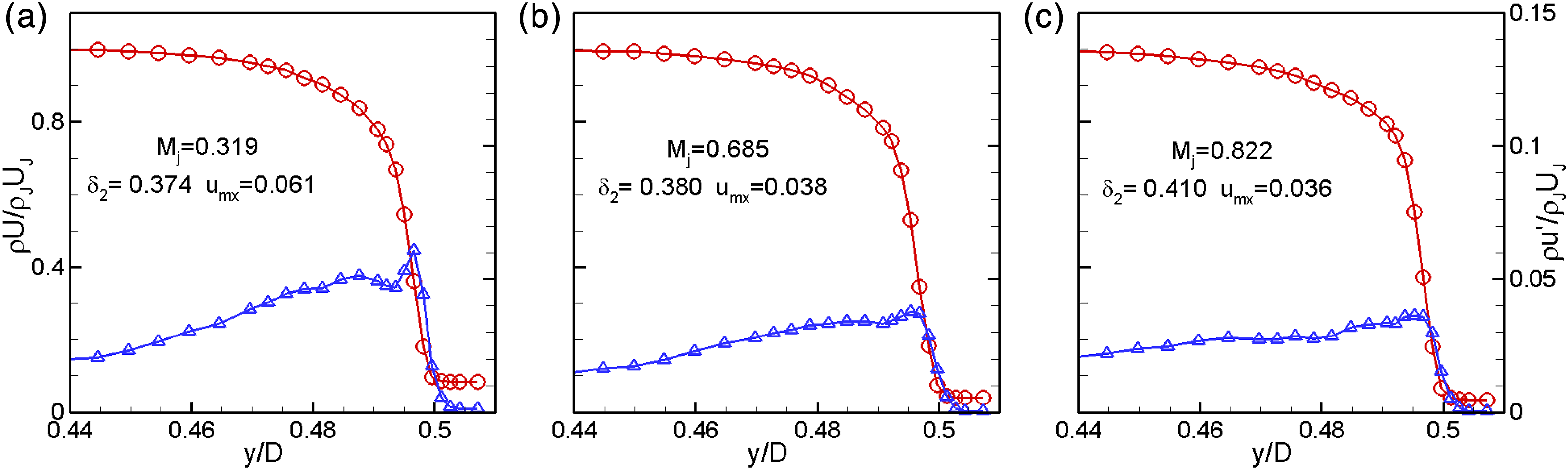

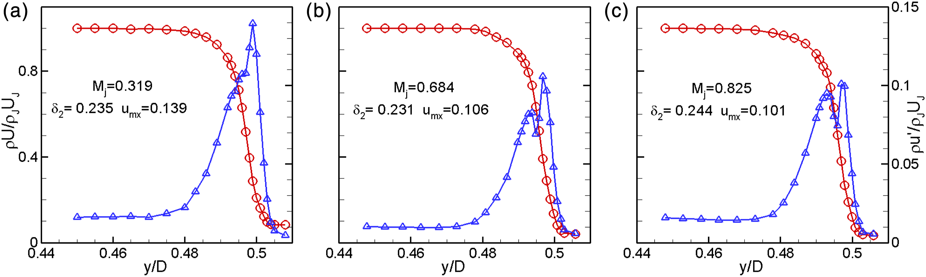
For the Conic nozzle in Figure 4, the mean velocity is characteristic of a turbulent boundary layer at all three M_J. It decays gradually over a long distance until a drop occurs near the wall. The shape factor (H₁₂ = δ₁/δ₂) turns out to be in the range 1.60–1.65; δ₁ and δ₂ are displacement and momentum thicknesses, respectively. The spectral content of the velocity fluctuations is broadband (sample velocity traces are shown later). From these considerations the boundary layer for the Conic nozzle is inferred turbulent. Note that the peak turbulence intensity is only 6% at M_J = 0.32 that drops considerably more with increasing M_J. These values, typical of nozzle flows with turbulent BL, are much lower than corresponding values in a flat-plate BL. Recall the turbulent BL’s issuing from pipes in⁴⁶ that showed peak intensities of 12% or more. The cylindrical pipe flow is akin to flow over a flat plate. It is possible that axial pressure gradients and compressibility effects cause the lower turbulence with the nozzles. In particular, nozzle flows experience favorable pressure gradient that can affect the stability characteristics of the BL. (Note that electronic noise contaminated the turbulence data in the jet core where the intensities were very small. This led to intensities in the core larger than actual and also some variations for data taken at different times. However, this effect at higher intensities within the BL was negligible).

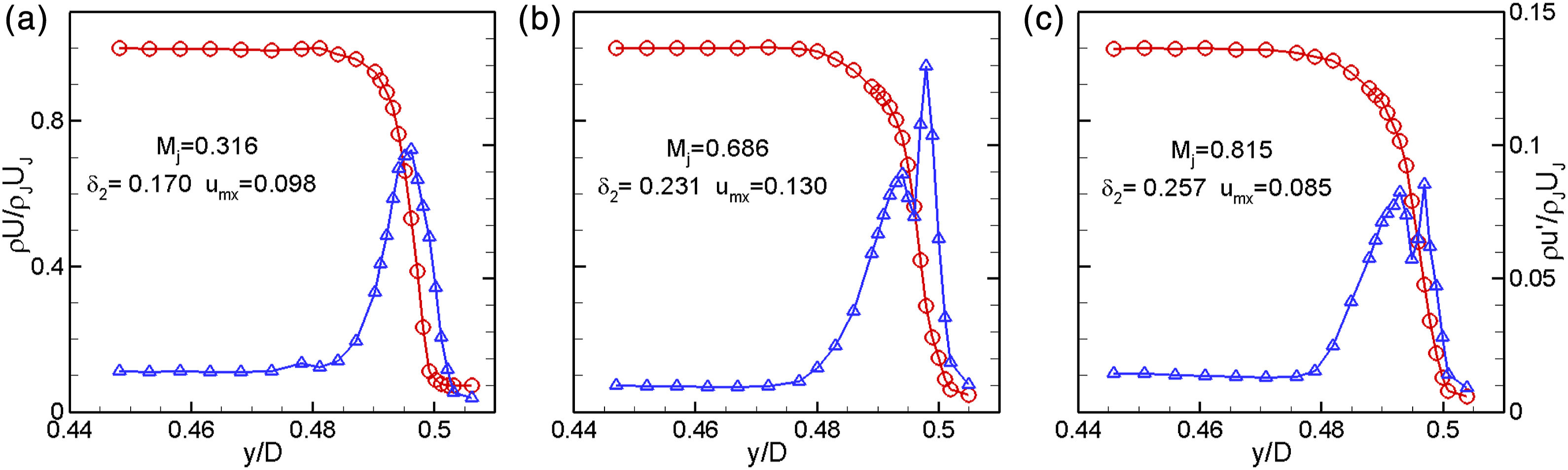
Corresponding data for the ASME design case are shown in Figure 5. Here, the mean velocity profile is flat within the core and the boundary layer is thinner. The turbulence intensities are conspicuously large. The mean velocity profiles bear similarity to the ‘Blasius-profile’; although the shape factor turns out to be about 2.0, smaller than that of a Blasius profile (2.59). In view of the large turbulence, possible effects from compressibility and pressure gradient and the fact that the profiles are measured downstream of the exit, deviations may not be unexpected. (The truncation in the integration at 98% point, necessitated by a temperature effect described shortly, contributed to the lower values of H₁₂. The displacement thickness δ₁ is underestimated more than the momentum thickness δ₂ due to such truncation. Also, the wall location, determined by extrapolation, can significantly affect δ₁. The data for δ₂ and peak turbulence intensity are more reliable and repeatable; δ_1, and hence H₁₂, are susceptible to changes in the integration procedure.) Thus, the mean velocity profile is considered laminar-like while the turbulence intensity is high, and this is the state referred to as ‘highly disturbed laminar’. The most conspicuous feature is the high turbulence intensity – much higher than that in a turbulent BL. Peak values in some cases exceed 15%. Often the u’-profile is characterized by a ‘double peak’ discussed further in the following. The highly disturbed laminar state for this nozzle persisted throughout the M_J range covered (up to M_J = 1, corresponding to Re_D ≈ 1.47 × 10⁶).

Corresponding data for the ASME long case are shown in Figure 6. Essentially similar characteristics are noted as with the ASME design nozzle and the BL is also inferred to be highly disturbed laminar. A distinction of the highly disturbed laminar BL (or nominally laminar BL in general) from a turbulent BL is in the velocity fluctuations away from the wall. In the latter case, the turbulence decay follows the slow increase in mean velocity away from the wall. Thus, with the Conic case the high-frequency fluctuations persist far away (∼0.10”), and this could be observed on an oscilloscope during data acquisition; comparatively, for the ASME design and long cases, the turbulent fluctuations dropped abruptly a short distance away from the wall (∼0.02”).

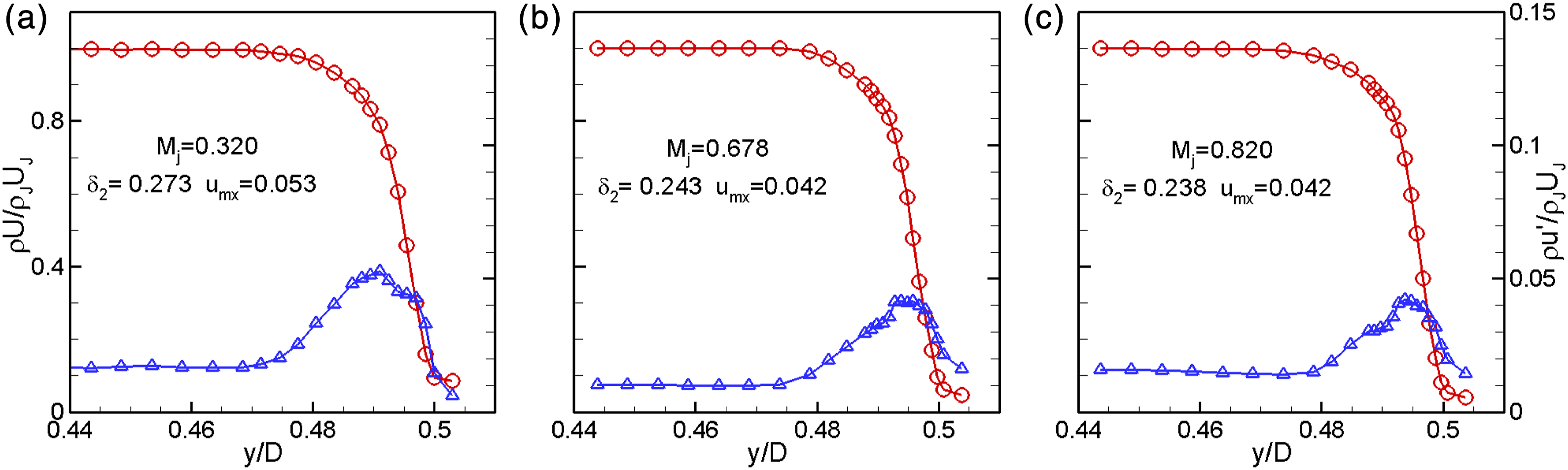
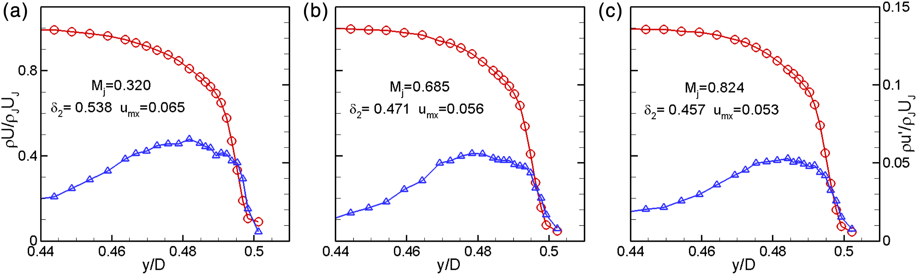
Referring back to Figure 3(c), it can be seen that the length of the flow path downstream of the K = 2 point is the shortest for the ASME short case. Hence a more laminar-like BL is expected. The mean-velocity profiles in Figure 7 do exhibit a thin laminar-like behavior as with the design and the long cases; however, the turbulence intensity is not large. This is a case similar to the Cubic nozzle of.¹⁵ Note that the turbulence intensity, even though small, drops to the core value within a short distance from the wall. The mean velocity increase and decay of turbulence do not persist far away from the wall as with the Conic case. Thus, the BL state is inferred to be nominally laminar but not highly disturbed laminar. On the other hand, for the short with extension (Sh-e) nozzle the BL is clearly turbulent (Figure 8). The trends are comparable to those of the Conic case in Figure 4.

Data at higher M_J (up to 1) were taken for all nozzles and the overall features of the profiles remained the same as discussed above. However, in all cases a near-wall ‘bump’ appeared in the mean velocity profile. The velocity was high over a small distance just outside the BL before relaxing to unity in the jet core. This was thought to be due to some thermal effect when the probe was close to the wall, leading to hot-wire errors (at transonic condition the static temperature is about 90°F colder than ambient); however, the exact reason remained unclear. The bump was less pronounced with thicker BLs. Its characteristics changed somewhat with different overheat ratio for the hot-wire. Furthermore, Pitot and static probe surveys did not produce the bump suggesting that it was indeed due to hot-wire errors. Because of sensor breakage issues it was not pursued further; an interested reader may look up¹ for more details. The bump, however, had a large impact on the integral thickness estimates; the truncation criterion for the integration became ambiguous. Thus, the results for M_J > 0.825 are not shown.

Characteristic boundary layer integral data as a function of M_J are shown in Figure 9. The five nozzles are identified in the legend of Figure 9(c). Momentum thickness versus M_J is shown in Figure 9(a). At large M_J, the values are small for the ASME design, long as well as the short cases. With turbulent boundary layers, it is large for the Conic and the ASME short-with-extension cases. It is the thickest for the last (Sh-e) case. At low M_J, the values for the Conic case are also small. Apparently, its boundary layer goes through transition around M_J = 0.3; a similar but sharper transition occurred at about the same M_J with a 1” diameter Conic nozzle.⁵

Figure 9.

Exit boundary layer characteristics versus M_J for the five nozzles. (a) Momentum thickness, (b) shape factor, and (c) peak turbulence intensity. Nozzle cases indicated in (c).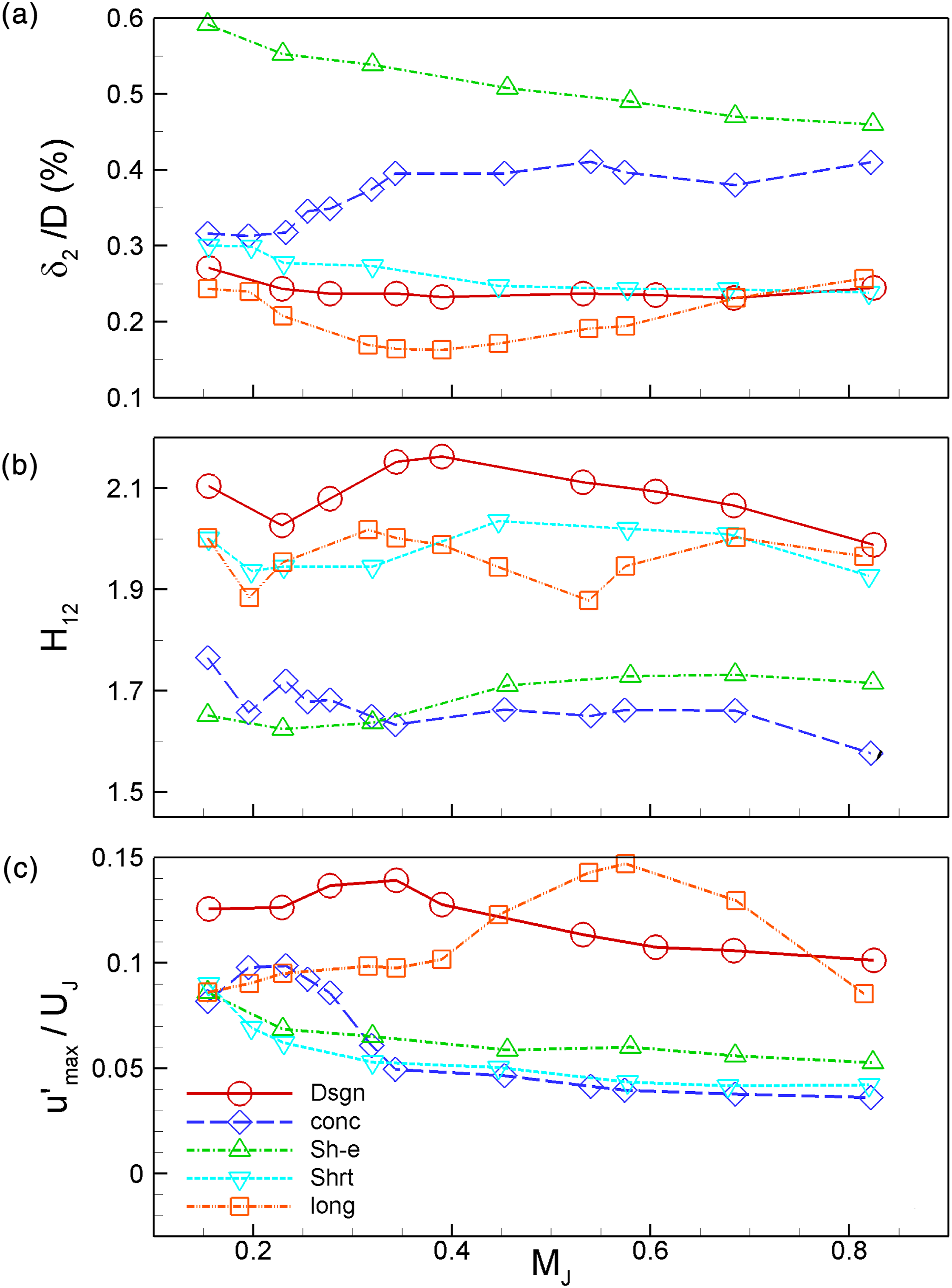

Corresponding shape factor (H₁₂) data are plotted in Figure 9(b). For the Conic case with turbulent boundary layer H₁₂ is relatively small and has values in the range of 1.6–1.65. For the ASME design case it is in the range of 2.0–2.15. Data for the Sh-e case is near the lower limit while that for the short case is near the higher limit. Just based on H₁₂ the boundary layer state may be ambiguous. Turbulence intensity, which also correlates with noise radiation, provides additional perspective for the BL state. Peak turbulence intensity data are shown in Figure 9(c). Over most of the M_J -range covered, the peak intensity is large for the design and long cases indicating a highly disturbed laminar state. For the Conic and Sh-e cases the peak intensity is low, as discussed before. For the ASME short case, the intensity is low, thickness small while H₁₂ is high.

Sample velocity traces obtained on the high-speed edge of the BL are shown for the ASME design, Conic and ASME short cases, in Figure 10(a)–(c), respectively. For the design case in (a) the fluctuation amplitudes are large. Note the large negative skewness of the signal, quantified in the legend (s = −1.55). Comparatively, the fluctuation amplitudes are small, and the value of s is close to zero for the Conic case in Figure 10(b). The velocity trace in Figure 10(c) for the ASME short case, somewhat surprisingly, shows a turbulent-like behavior with high-frequency content. However, the skewness is still substantially negative and from the mean velocity profile and H₁₂ value it is also designated as a nominally-laminar case. It is neither fully laminar nor highly disturbed laminar.

Figure 10.

Time traces of hot-wire signal at about 94% velocity point in the boundary layer for (a) Dsgn, (b) Conic and (c) Shrt cases. Radial location (y/D), Mean velocity (U/U_J), turbulence intensity (u’/U_J) and skewness (s/u’³) are indicated in legends; M_J = 0.31.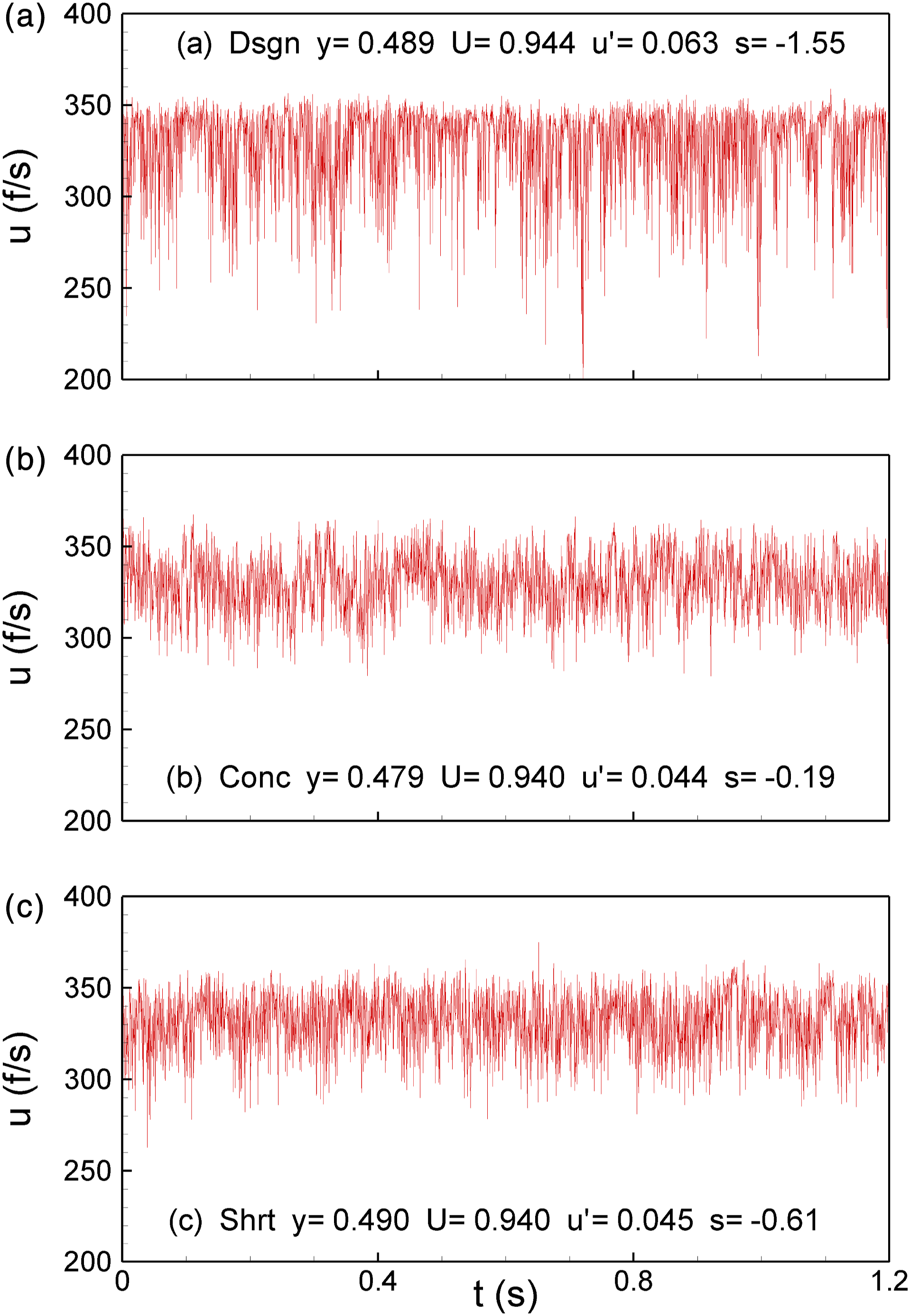

An explanation for the dual-peak turbulence profiles with highly disturbed laminar BL is as follows. Large negative spikes mark the velocity traces on the high-speed edge yielding large negative s, while large positive spikes occur on the low-speed edge yielding large positive s (shown in⁵). These are indicative of an unsteady transitional state with high intermittency. The negative spikes occur due to intermittent transfer of low momentum fluid from the low-speed side to the high-speed side and vice versa. The changeover of the skewness across the BL is commensurate with the dual peaks in the turbulence intensity profiles (Figures 5 and 6). Either the negative or the positive spikes result in high rms value with a minimum occurring in the middle at the changeover location.

With regards to the BL states a question came up. Recalling that the measurements are done 0.030″ downstream of the nozzle lip, the question was: did the boundary layer inside the nozzle bore the same characteristics or a transition occurred after the boundary layer exited the nozzle? Velocity traces were inspected 0.2″ upstream; (this had to be done by intruding the probe through the flow on the other side of the nozzle, and thus it was done only at the low value of M_J = 0.31). For all cases, the characteristics of the velocity traces were the same as seen downstream. Thus, the nominally-laminar or turbulent state originated from inside the nozzle.

Therefore, for M_J > 0.35, a nominally-laminar state exists for the ASME design, long and short cases. Among the three, the design and the long cases have the highly disturbed laminar state. Clearly a turbulent state exists for the Conic and the short-with-extension cases. Note that the states are persistent with the respective nozzles throughout the Mach number range covered. At low M_J the state may vary for some of the nozzles, however, the focus here is at high M_J where the noise measurements are performed. The state for the ASME short case is inferred to be nominally-laminar although the peak turbulence intensity is low and comparable to that of the turbulent cases. The behavior remains somewhat puzzling also because the BL thickness is comparable to that of the ASME design case even though the latter has a longer cylindrical section. The BL states for all nozzles studied are listed later in Table 1.

Table 1.

Boundary layer characteristics and state (NL = nominally laminar; HDL = highly disturbed laminar).

Nozzle	M_J range	δ₂/D (%)	H ₁₂	u’_mx/U_J	BL state	Noise
Conic	<0.25	∼0.32	1.65–1.75	∼0.10	NL	--
Conic	>0.35	∼0.40	1.55–1.60	0.035 – 0.05	Turbulent	Low
ASME design	>0.2	∼0.25	2.00–2.15	0.110 – 0.140	HDL	High
ASME long	>0.2	0.15 – 0.25	1.90–2.00	0.100 – 0.150	HDL	High
ASME sh-e	>0.2	0.45 – 0.55	1.65–1.70	0.060 – 0.070	Turbulent	Low
ASME short	>0.2	0.25 – 0.30	1.90–2.00	0.050 – 0.070	NL	Intermediate
SMC	0.35–0.55	0.12 – 0.20	1.95–2.05	0.100 – 0.145	HDL	--
SMC	>0.6	∼0.20	1.90–2.00	∼0.04	NL	Intermediate
SMC+	>0.3	∼0.60	1.45–1.55	0.035 – 0.050	Turbulent	Low

An observation on nozzle size effect is made here based on the present and earlier results of.^5,45 The differences between the ASME design and the Conic cases are somewhat less pronounced with the 2″ nozzles compared to the 1″ nozzles in.⁵ For example, in,⁵ the transition to turbulence with the Conic nozzle around M_J =0.3 was much sharper, and the difference in peak turbulence between the two cases was larger. Recall that in⁴⁵ noise difference for a pair of 2″ nozzles (Conic and ASME) was minimal while significant difference occurred for a pair of 1.5″ nozzles. Thus, it appears that the noise difference may disappear for even larger nozzles, that is, the highly disturbed laminar state with the ASME nozzle may cease to exist when the Re_D is higher. The upper limit of Re_D for this to occur would likely vary from facility to facility.

Jet noise data

As stated in the Experimental Procedures, the noise measurements were performed in the GRC AAPL, a high-quality anechoic facility within NASA. Because of busy facility schedules, only the ASME design, short-with-extension and the Conic nozzles were tested. The data were acquired for cold flows covering a range of M_J. These spectral data were corrected for atmospheric attenuation and referenced to 1-foot distance from the nozzle; sound pressure level (SPL) power spectral density in dB per Hz are presented as a function of Strouhal number (fD/U_J, U_J = jet velocity at nozzle exit). Figure 11(a) compares the spectra between the ASME design and the Conic cases for a polar location, θ = 90°. A similar trend as seen in¹⁵ and⁵ is confirmed. The noise amplitudes are unambiguously larger on the high-frequency end for the ASME design case. The same data are plotted in Figure 11(b) in 1/3^rd-octave format. Overall, an unmistakable similarity with the spectral comparison in Figure 1 can be seen. With other possibilities (e.g., effects of upstream rig noise, core turbulence and lip thickness) ruled out,^5,43 it is logical to infer that the anomaly discussed in the Introduction must be due to a difference in the initial BL state.

Figure 11.

Comparison of sound pressure level (SPL) spectra between Conic and design cases; all noise data are measured at a distance of 75D from the nozzle exit. (a) PSD referenced to 1-ft distance, (b) same data in 1/3^rd-octave format.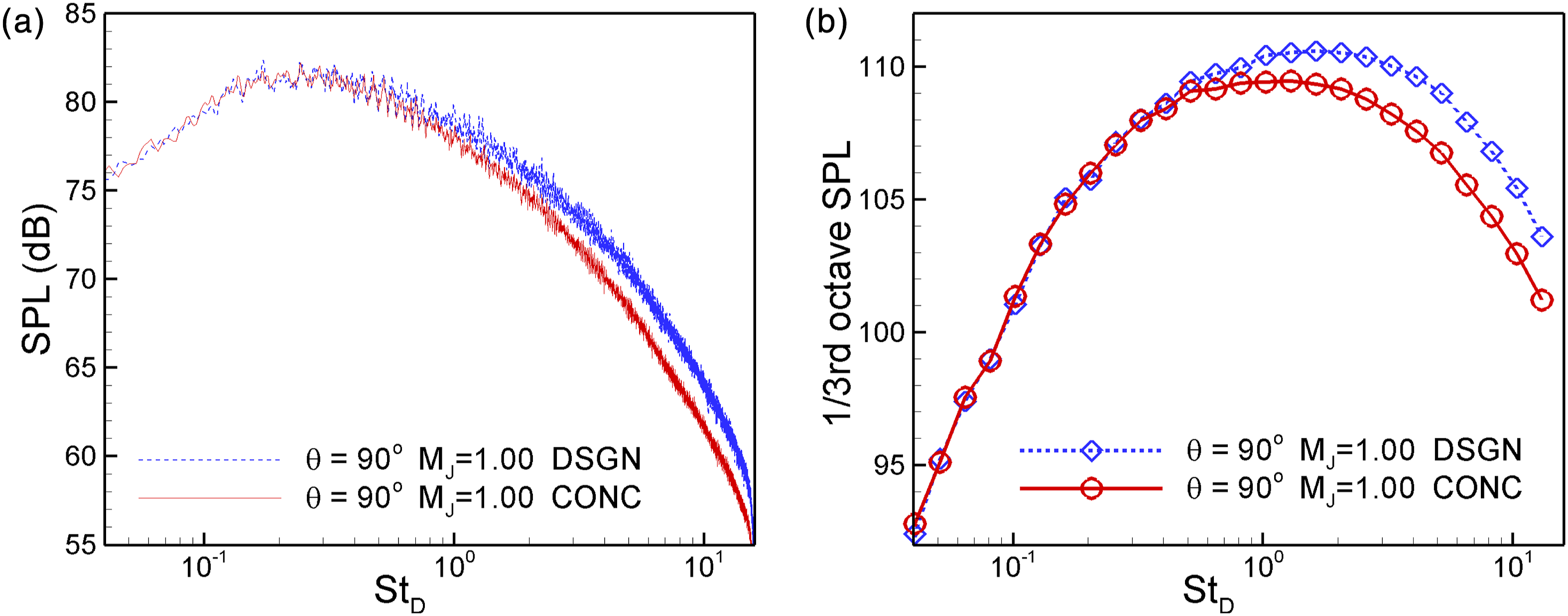

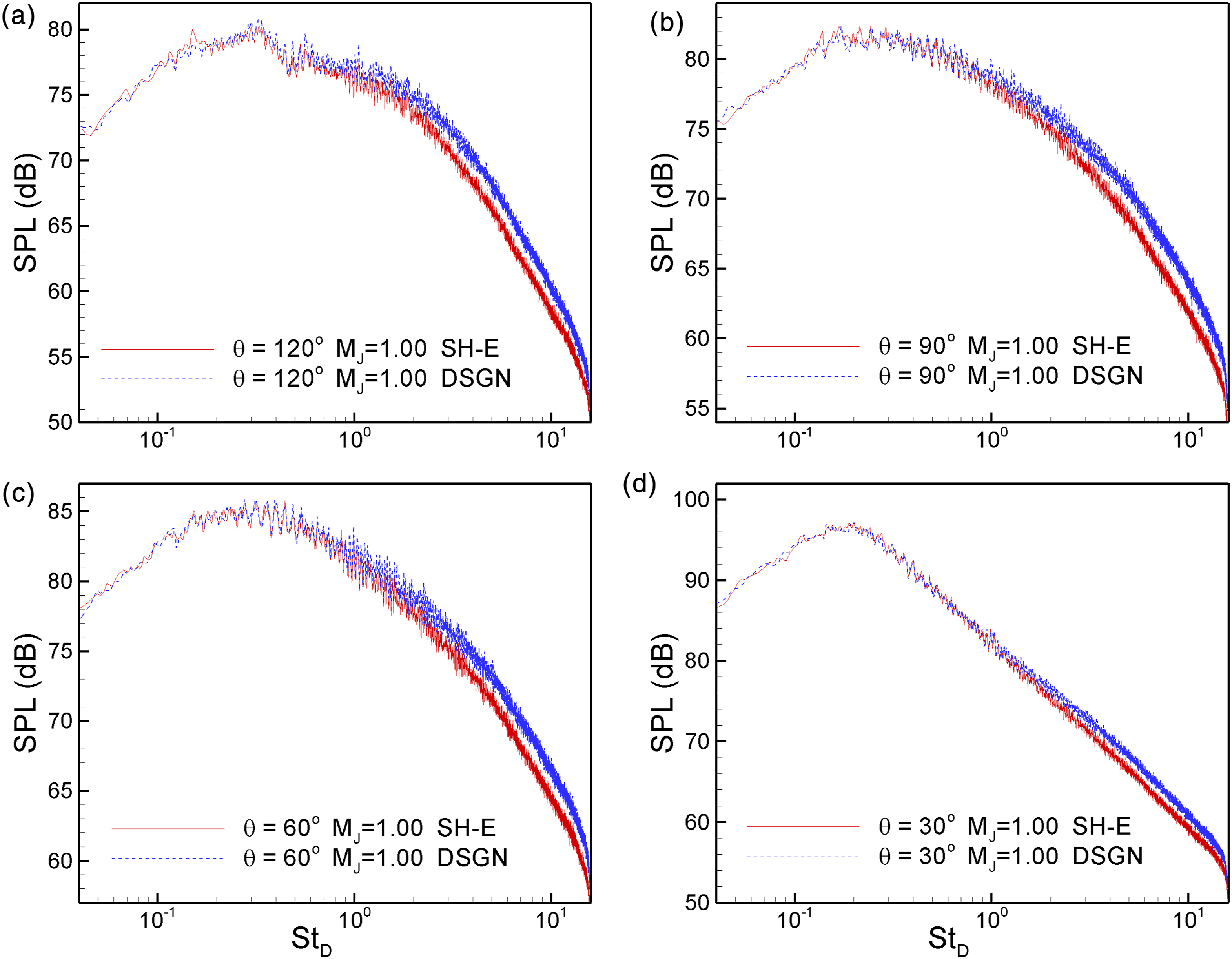
Some further comparisons of the SPL spectra are made here. Figure 12 compares the data between the ASME design and short-with-extension cases for four values of M_J. Recall that the Sh-e case also has a turbulent BL and a similar amplitude difference at high-frequencies, as seen in Figure 11, can be seen at all M_J. Figure 13 shows that the amplitude difference also occurs at other polar locations and the difference is more pronounced at larger values of θ. A similar observation was made from LES data in.⁴¹ Directivity plots, overall sound pressure level (OASPL) versus θ, are shown in Figure 14(a). The noise amplitude is larger for the ASME design case over most of the θ-range; the difference is seen to vanish at the lowest end of the range. Directivity for partial OASPL (amplitudes integrated over 20–40 kHz where the noise difference is the largest) are shown in Figure 14(b). These data further demonstrate the impact of the boundary layer state on radiated noise.

Figure 12.

Comparison of SPL spectra between the Dsgn and Sh-e cases at θ = 90° for four jet Mach numbers: (a) M_J = 1.00, (b) M_J = 0.96, (c) M_J = 0.83 and (d) M_J = 0.66.

Figure 13.

Comparison of SPL spectra between the Dsgn and Sh-e cases at M_J = 1.00 for four polar locations: (a) θ = 120°, (b) θ = 90°, (c) θ = 60° and (d) θ = 30°.

Figure 14.

Directivity plots. Data for three nozzles as indicated at three values of M_J: (a) OASPL versus θ (b) Partial OASPL (integrated over 20–40 kHz range) versus θ.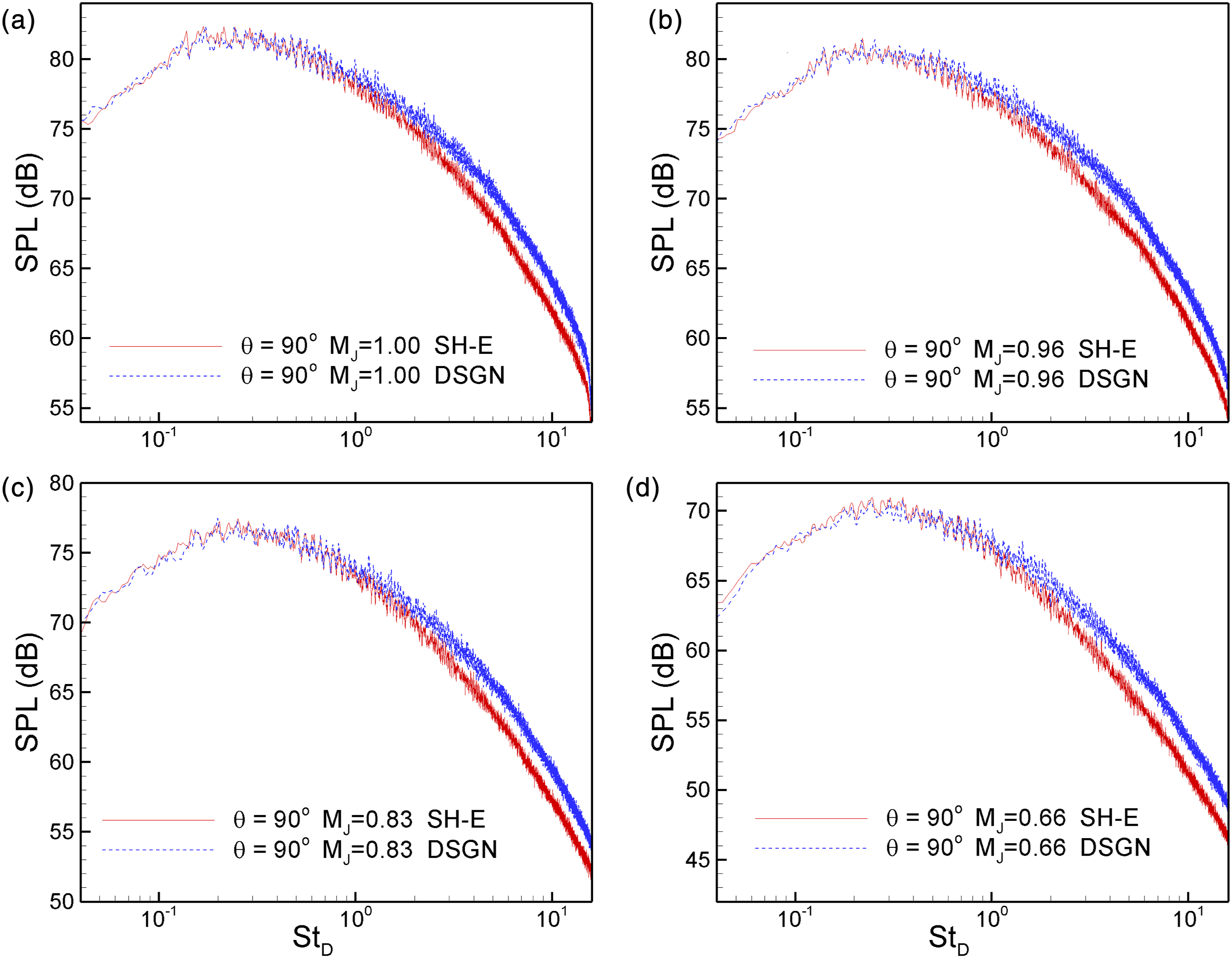

Recall that the ASME short case showed a large shape factor but a low peak turbulence intensity. What happens with noise for this case? Unfortunately, as stated before noise was not measured in the AAPL for this case. However, qualitative noise measurements were done earlier in the CW17 facility and reported in.¹ Amplitudes for this case fell between those for the ASME design case (high) and the ASME Sh-e case (low). Thus, it exhibited some increased noise but not as much as the design or the long cases. The SMC nozzle exhibits a similar BL state as the ASME short case in a certain M_J range; its noise characteristics are examined in the next subsection.

Schlieren flow visualization images are shown in Figure 15 to gain some insight into the flowfield differences that lead to the noise difference. Images are compared at four values of M_J between the ASME design and the short-with-extension cases. An inspection reveals that the shear layers of the ASME design case contain relatively more organized coherent structures. Comparatively the shear layers of the Sh-e case, with turbulent BL, are more diffused. A similar difference was noted by schlieren visualization between laminar (untripped) and turbulent (tripped) jets in a past work.¹⁹ LES studies, reviewed in the Introduction, also show that the dynamics of the organized coherent structures (instability waves) are responsible for higher shear layer turbulence and hence a resultant higher noise for the laminar-like boundary layer cases. Before parting, it is noted that a similar difference in organized shear layer structures appears to persist at the supersonic condition covered in Figure 15. Thus, the BL states inferred for these nozzles are likely to persist into the supersonic regime.

Figure 15.

Schlieren pictures at four jet Mach numbers as indicated. Top row for Dsgn case, bottom row for Sh-e case.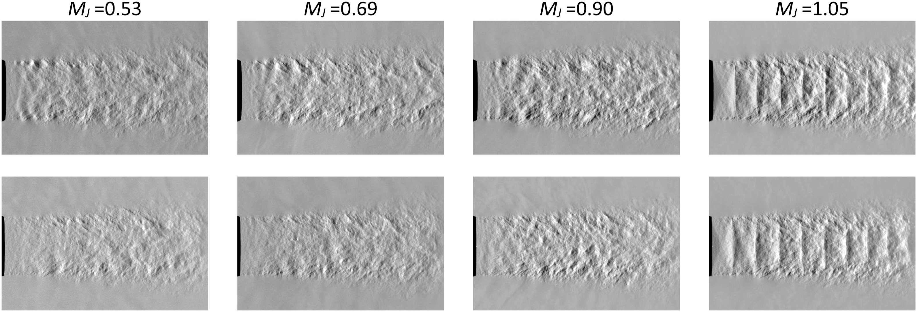

Results for the SMC nozzle

The ‘SMC000’ (Small Metallic Chevron nozzle, baseline case) has been used in various investigations of flow and noise for isolated jets as well as complex configurations.^13,50 Some of these experimental configurations, involving either free jets or jet-surface interaction, have been explored numerically using LES codes at the Naval Research Laboratory (Code JNRE;⁵¹) as well as at the NASA Ames Research Center (Code LAVA;⁵²); see also.^53,54 The LAVA simulation⁵² and the corresponding experiment involved an extension pipe added upstream of the nozzle (Figure 2(e)). The simulation in,⁵¹ on the other hand, involved the usual installation of the nozzle with a convergent adapter attached to the jet facility. The exit boundary layer characteristics of the nozzle with and without the upstream pipe were not measured before. This was carried out and the results presented in.² Excerpts pertinent to this paper are presented in the following; an interested reader may find more details of the flow field evolution in the cited report.

The two nozzle configurations, without and with the upstream pipe, are referred to as ‘SMC’ and ‘SMC+’, respectively (Figure 2(d) and (e)). The SMC nozzle, with 2″ exit diameter, is convergent with a 5° half angle at the exit; its coordinates can be found in.² The upstream pipe with the SMC+ has a slightly larger internal diameter (2.25″). The convergence from 2.25″ to 2″ diameter is mild and thus the turbulent boundary layer developed over the 12″ length remains turbulent at the nozzle exit. The BL momentum thickness (δ₂) variation is shown in Figure 16 that exhibits small values for the SMC measuring 0.001D – 0.002D over the M_J -range covered. The value of δ₂ for the SMC+ nozzle is high throughout and at least three times larger. Corresponding peak turbulence intensity data are shown in Figure 17. One notes that the levels are low for the SMC+ case but the SMC case exhibits large values within the M_J range of 0.33–0.55. The large turbulence is indicative of a highly disturbed laminar state as with the ASME design and long cases.

Figure 16.

Exit boundary layer momentum thickness versus M_J for SMC nozzle without and with 12” long pipe upstream; SMC+ denotes the case with the pipe.

Figure 17.

Maximum turbulence intensity in the exit boundary layer versus M_J for the SMC and SMC+ cases.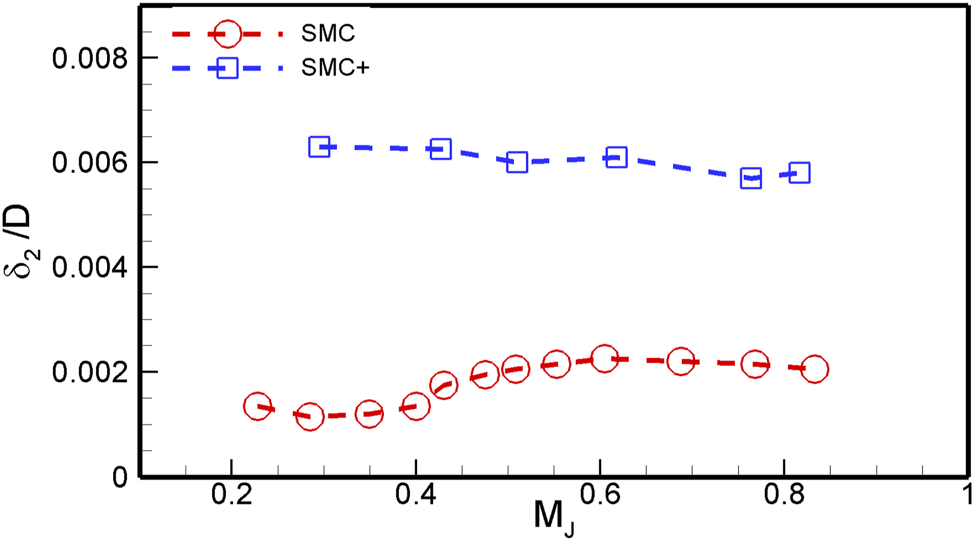

From the data of Figure 17, one may be tempted to conclude that with increasing M_J the SMC nozzle BL goes through a transition, becoming highly disturbed laminar in the M_J range of 0.33–0.55 and then turbulent for M_J > 0.6. Once turbulent the peak intensity is the same as that of the SMC+ case. That this notion is incorrect becomes apparent from the δ₂ data in Figure 16; the SMC BL thickness continues to be small and there is no jump to indicate a transition has taken place. The velocity profiles in Figure 18 confirm that the BL has not transitioned for the SMC case. The profiles for SMC and SMC+ cases are compared at M_J ≈ 0.76 where the high turbulence with the SMC case has subsided (Figure 17). While the peak turbulence is about the same for the two configurations, the mean velocity profiles are vastly different. The profile for the SMC+ case (Figure 18(b)) is clearly turbulent (compare, e.g., with the Conic case in Figure 4). It has the prolonged rise of the mean velocity, accompanied by a prolonged decay of turbulence, away from the wall. In contrast, the BL is thin and laminar-like for the SMC case (Figure 18(a)). The shape factor H₁₂, shown in the legends, is about 1.9 and 1.5, for the SMC and SMC+ cases, respectively. Thus, a nominally-laminar state exists for the SMC case at M_J ≈ 0.76. However, the peak turbulence is low and comparable to that in the turbulent case. The condition is similar to the ASME short nozzle discussed in the previous section.

Figure 18.

Mean velocity (red, circles) and turbulence intensity profiles (blue triangles) for: (a) SMC, M_J = 0.768; (b) SMC+, M_J = 0.764.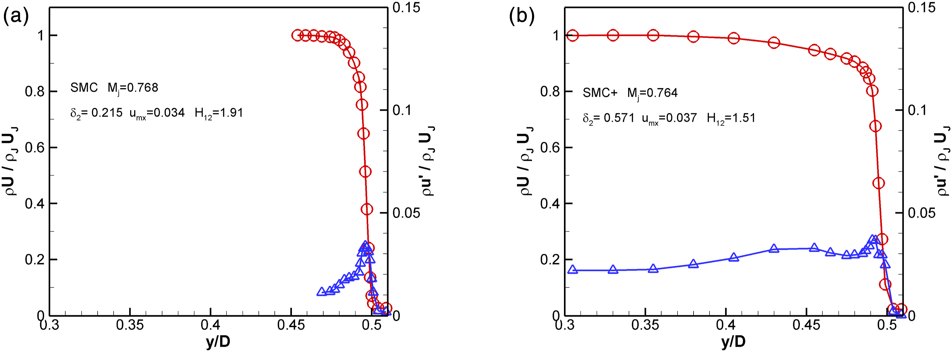

Corresponding profiles for the SMC and SMC+ cases are compared in Figure 19 at M_J = 0.43, a condition where the peak turbulence intensity was the largest for the SMC case (Figure 17). The sharp peak in the turbulence profile (Figure 19(a)) is conspicuous and the boundary layer is thin. This is a highly disturbed laminar state as with the ASME design and long cases. Here, the highest intensity occurs on the lower speed side where ρU/ρ_J U_J is about 0.27. The tendency for a dual-peak distribution is also apparent. Corresponding data for the SMC+ case at M_J ≈ 0.43 (Figure 19(b)) clearly exhibit a fully turbulent state, as at the higher M_J in Figure 18(b).

Figure 19.

Mean velocity (red, circles) and turbulence intensity profiles (blue triangles) for: (a) SMC, M_J = 0.426; (b) SMC+, M_J = 0.427.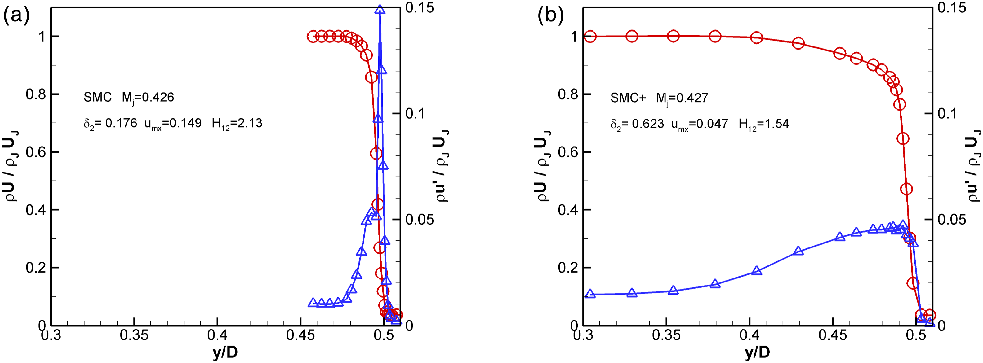

A brief review shows that high peak turbulence, as in the present highly disturbed laminar cases, were encountered in several previous studies, e.g., a level of 0.172 in.²¹ However, there does not seem to be much data on turbulent BLs for convergent nozzles exhibiting low levels as in the present experiments. The BLs in both⁴⁶ and⁴¹ were turbulent; the former reported levels in the range 0.120 – 0.145 while a level of about 0.110 was measured in the companion experiment of.⁴¹ Both studies, however, involved long straight sections, i.e., pipe-like geometry rather than convergent nozzles. In the experiment of,⁴² a long ‘conic’ convergent nozzle was apparently used that may have yielded a turbulent BL; peak levels of about 0.070 can be seen in their turbulence intensity profiles. It is important to note here that BL tripping with the ASME design nozzle also reduced the peak turbulence level drastically; (data not shown here for brevity but can be found in.¹) For example, the peak level of 0.135 at M_J = 0.69 (Figure 5(b)) dropped to 0.040 when the BL was tripped. Contrast this to BL tripping effect in pipe-like nozzles or a 2-D planar BL. Tripping of a 2-D BL by Batt,¹⁸ perhaps as expected, increased peak turbulence level, from 0.02 to 0.12. An increase in peak turbulence by BL trip also occurred for a pipe-like nozzle flow, in the experiment of Moore.³⁰ Low turbulence levels, measured in all of the turbulent BL cases of the present experiments, are characteristic of convergent nozzle flows and must be due to favorable pressure gradients.

Far field noise data for the SMC and SMC+ configurations are compared in Figure 20 at approximately the same conditions of Figures 18 and 19. (These noise data were obtained and provided by colleague Dr James E. Bridges. The data were taken in the AAPL in 2020 while preparing for another experiment. Unlike the noise data in Figures 11–13 that were referenced to 1-foot distance, these are referenced to 100D. Also, these data were first converted to 1/12^th octave format and then presented as PSD per unit Strouhal number. No attempt was made to convert these in the same format as in the earlier figures since the comparisons discussed in the following are adequate for the purposes of this paper.)

Figure 20.

Comparison of SPL PSD between the SMC and the SMC+ cases at two jet Mach numbers (M_J) and two polar locations (θ) as indicated. PSD referenced to 100D is shown versus Strouhal number based on diameter (D).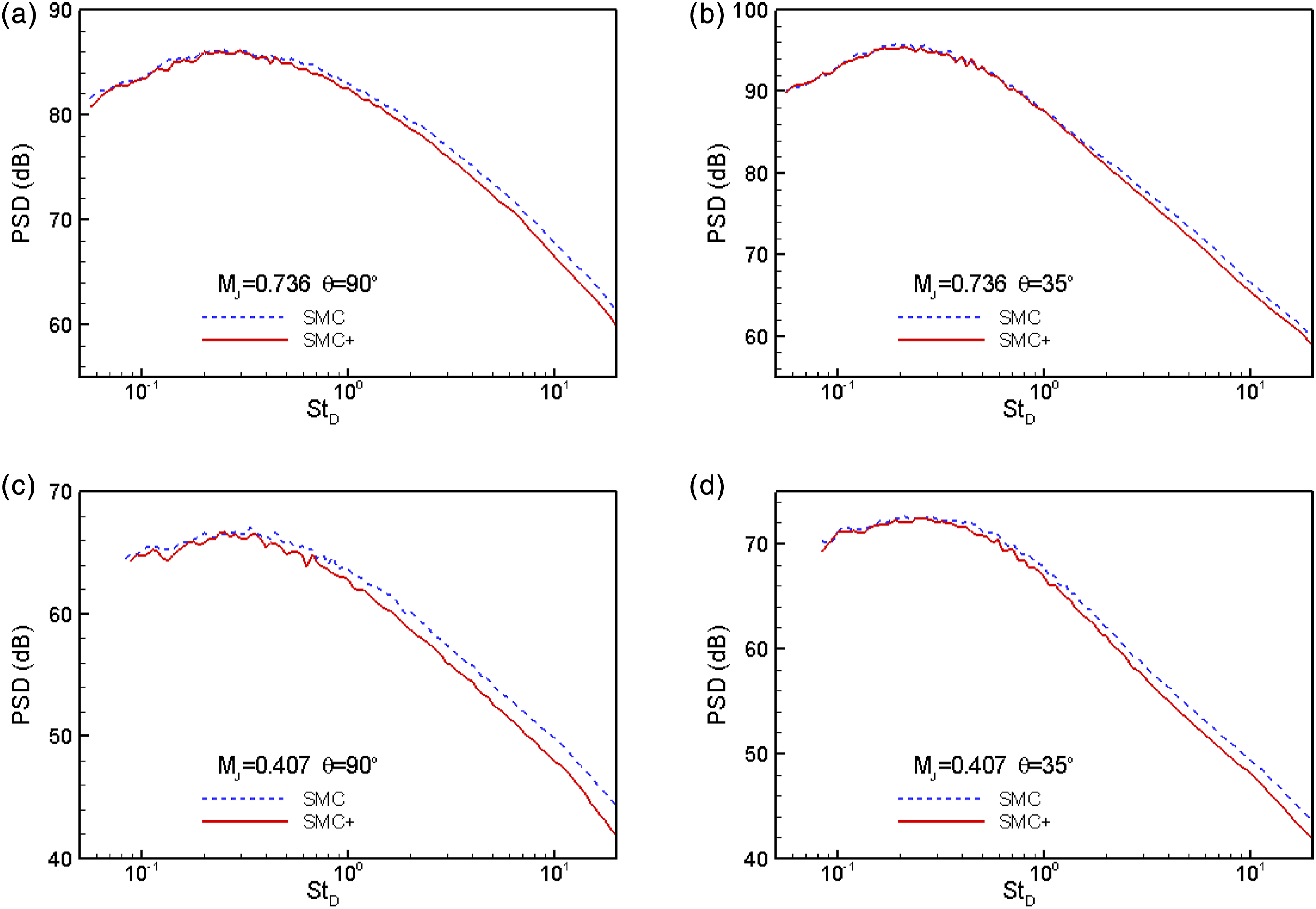

Figure 20(a) and (b) are for M_J = 0.736 where the SMC case BL is nominally-laminar but the peak turbulence is low and comparable to that of the SMC+ case. Figure 20(c) and (d) are for M_J = 0.407, where the peak turbulence for the SMC case is high and the BL is highly disturbed laminar. The BL is turbulent for the SMC+ case at both values of M_J. Figure 20(a) and (c) are for a sideline direction (θ = 90°) and Figure 20(b) and (d) are for a peak noise radiation direction (θ = 35°). It is apparent that in all conditions the noise amplitudes are somewhat larger for the SMC case. However, the increase is relatively more for the highly disturbed laminar case at M_J = 0.407.

Thus, even with the nominally-laminar BL with low peak turbulence (at M_J = 0.736) there is a noise increase relative to a turbulent BL. This is likely to be a BL thickness effect. As observed in,^{37,41,45 and 46} a thicker BL produces less noise. Here, it should be emphasized that this is not simply a result of a smaller effective diameter. Noise intensity at a given distance scales as square of the diameter ratio. As long as the core velocity remains the same a difference in jet diameter due to BL thickness should have negligible effect on noise. For example, between the SMC and the SMC+ cases (taking effective diameter = D – 2δ₁) it is estimated that only a 0.08 dB difference may be expected at a fixed distance. The noise difference on the high-frequency end for M_J = 0.736 (Figure 20(a) and (b)) is perceptible and about 1 dB. From a similar comparison between the Conic and the ASME design nozzles (Figures 4, 5 and 9) only about 0.03 dB noise difference due to BL thickness may be expected whereas the actual differences are about 2 dB (Figure 11). The BL thickness effect on noise comes from a change in the stability characteristics of the jet’s shear layer. As shown in prior studies, e.g.,^37,41,46 a thinner shear layer leads to larger amplification of Kelvin-Helmholtz waves at higher frequencies. This leads to higher turbulence and hence higher noise on the high-frequency end of the spectra.

The observations in the previous paragraph are supported by an analysis of the noise data in the format used in.⁴⁶ The same data of Figure 20 are nondimensionalized by the initial momentum thickness instead of the nozzle diameter and plotted in Figure 21 (i.e., amplitudes at 100δ₂ are plotted vs Strouhal number based on δ₂). Figure 21(a) and (b) show that such a normalization collapses the data on the high-frequency end, particularly when measured in the peak noise radiation direction (smaller θ). A similar collapse of noise spectra was noted in⁴⁶ for three different BL thicknesses. This basically implies that the initial BL thickness dictates the high-frequency noise amplitude (whereas the diameter D dictates lower frequency spectral amplitudes). Hence a thinner BL for a given diameter produces higher spectral amplitudes on the high-frequency end.

Figure 21.

Same data of Figure 20 shown versus Strouhal number based on δ₂ (δ₂ = BL momentum thickness) and referenced to 100δ₂.

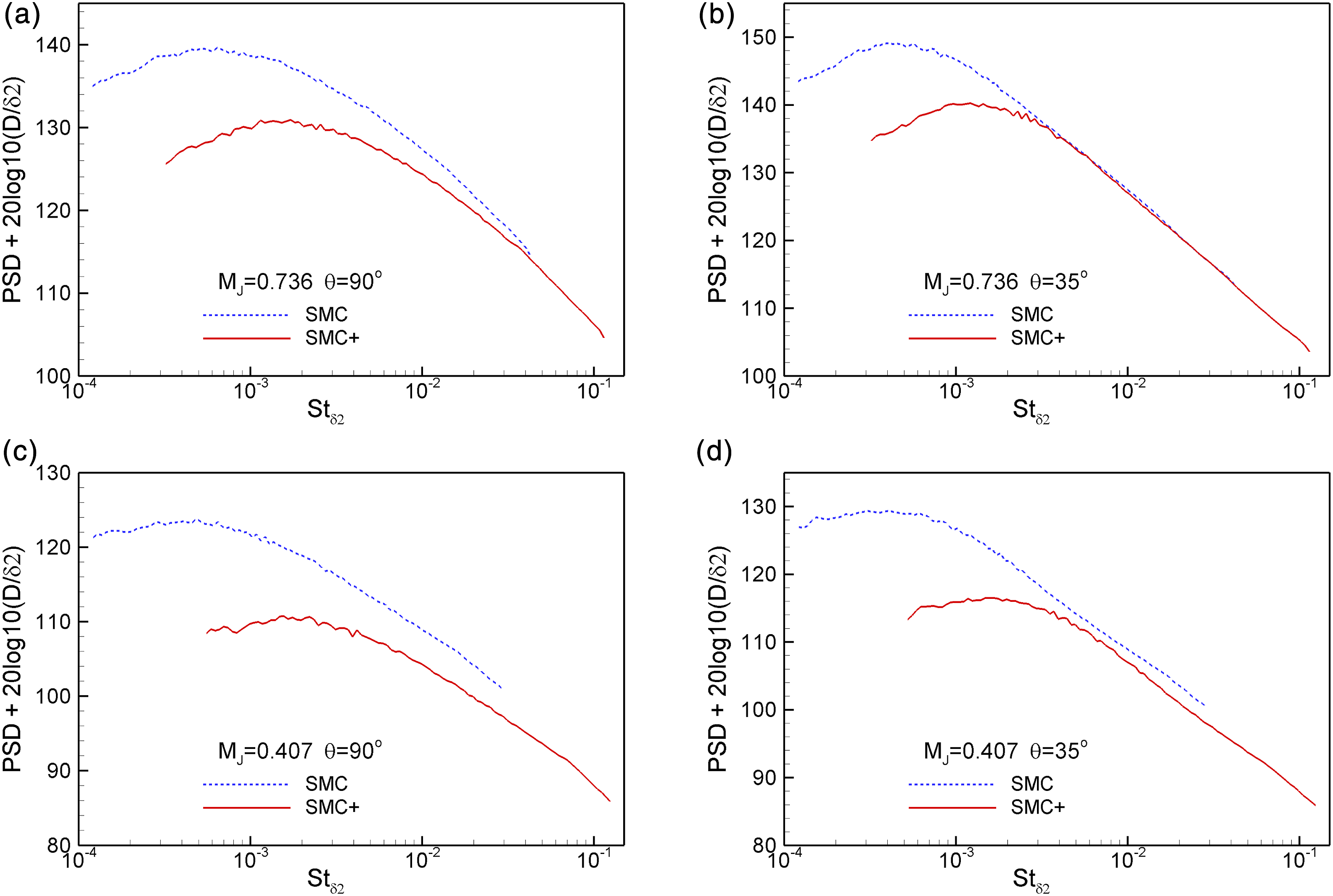
However, a lack of collapse in the noise amplitudes is seen between the SMC and SMC+ cases in Figure 21(c) and (d). The amplitudes are larger for the SMC case at M_J = 0.407 when the initial BL is highly disturbed laminar. This is due to the additional effect of the large initial turbulence. Thus, a nominally-laminar case with thinner BL produces more noise relative to a turbulent BL but the effect is accentuated when the initial turbulence intensity is large as in the highly disturbed laminar case.

Table 1 summarizes the BL states and noise characteristics of all nozzles of the current study. Note that the measurements covered the approximate M_J range of 0.15 – 1.00. Low and high noise pertains to high-frequency end of the SPL spectra with differences in the order of 2 dB in amplitudes. An inspection makes it apparent that the BL state may be ambiguous based on a single parameter such as H₁₂. The peak turbulence intensity as well as the mean velocity and turbulence intensity profiles must also be considered to assess the BL state.

LES results

As stated in the Introduction, LES studies were performed at NRL for the SMC and SMC+ cases. Details of the computational procedures and results can be found in.³ Here key results are discussed briefly. Instantaneous Mach number contours, at M_J = 0.736, are shown in Figure 22(a) and (b) for the SMC and the SMC+ cases, respectively. The dark red band of contours showing maximum Mach number in either case occurs near the nozzle exit. Corresponding BL profiles at the exit of the nozzles are compared in Figure 23. These profiles may be compared with the experimental data in Figure 18. Overall, the comparisons for both mean velocity and turbulence intensity are good. The SMC+ clearly shows a turbulent BL while it is nominally-laminar for the SMC case.

Figure 22.

LES results from Ref. [3]. Instantaneous Mach number distribution at M_J = 0.736: (a) SMC, (b) SMC+.

Figure 23.

LES results from.³ Comparison of the nozzle-exit velocity and turbulence intensity profiles for the SMC (green lines) and SMC+ (red lines) cases at M_J = 0.736.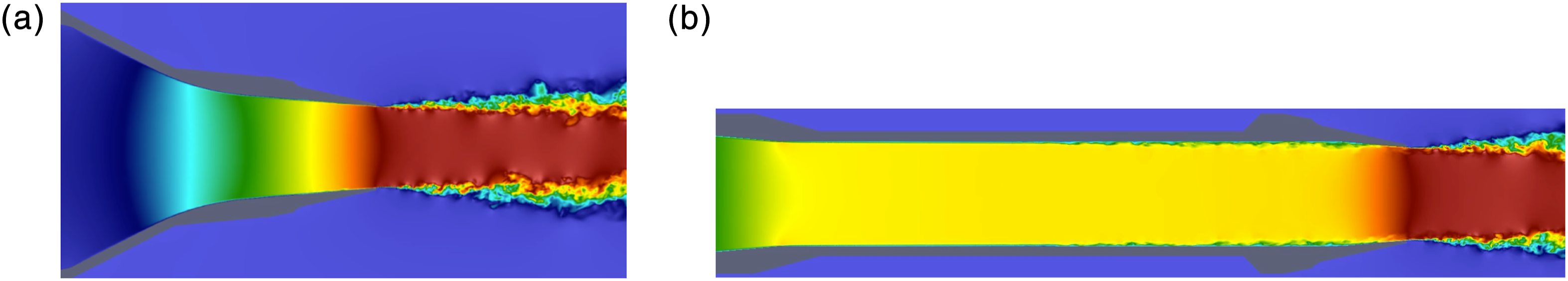

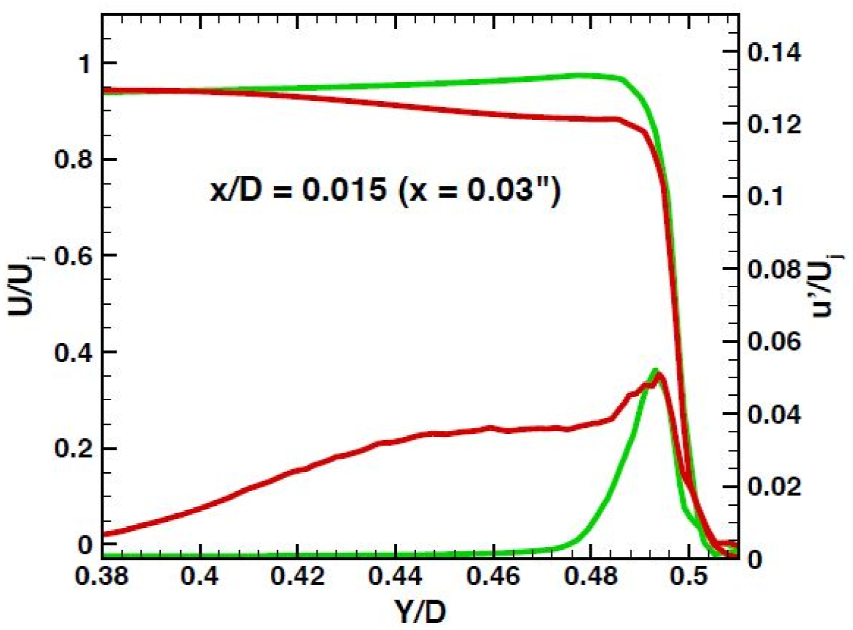
An insight is gained from the details of the calculations for the SMC+ case shown in Figure 24. Figure 24(a) shows contour plot of instantaneous velocity near the wall. The transition of laminar to turbulent state is observed around x/D = −3.5. A scrutiny of the turbulence intensity contours on a cross-sectional plane, shown in Figure 24(b), show a region of high turbulence (red) around the same location (x/D ≈ −3.5). The turbulence intensity profiles at different axial locations are compared in Figure 24(c). These data illustrate the role of the transition region possibly explaining the various BL states at the nozzle exit. The peak turbulence intensity is high in the transition region, as in a highly disturbed laminar state. It drops to a lower value when the BL becomes turbulent. A further drop in the peak intensity occurs as the BL passes through the convergent section near the exit. Dr Liu explored these behaviors with varying wall roughness that shifts the location of the transition region. Thus, depending on the wall roughness and Mach number the transition region may occur at different locations along the pipe. When the location coincides with the nozzle exit a highly disturbed laminar BL is obtained. An interested reader may find further details in.³

Figure 24.

LES results from³ for the SMC+ case at M_J = 0.736. (a) Instantaneous velocity fluctuations near the nozzle surface. (b) Turbulence intensity contours inside the nozzle boundary layer. (c) Turbulence intensity radial profiles at three axial locations; the red line is at x = −3.4D, green line at x = −1.0D and blue line at x = 0.015D.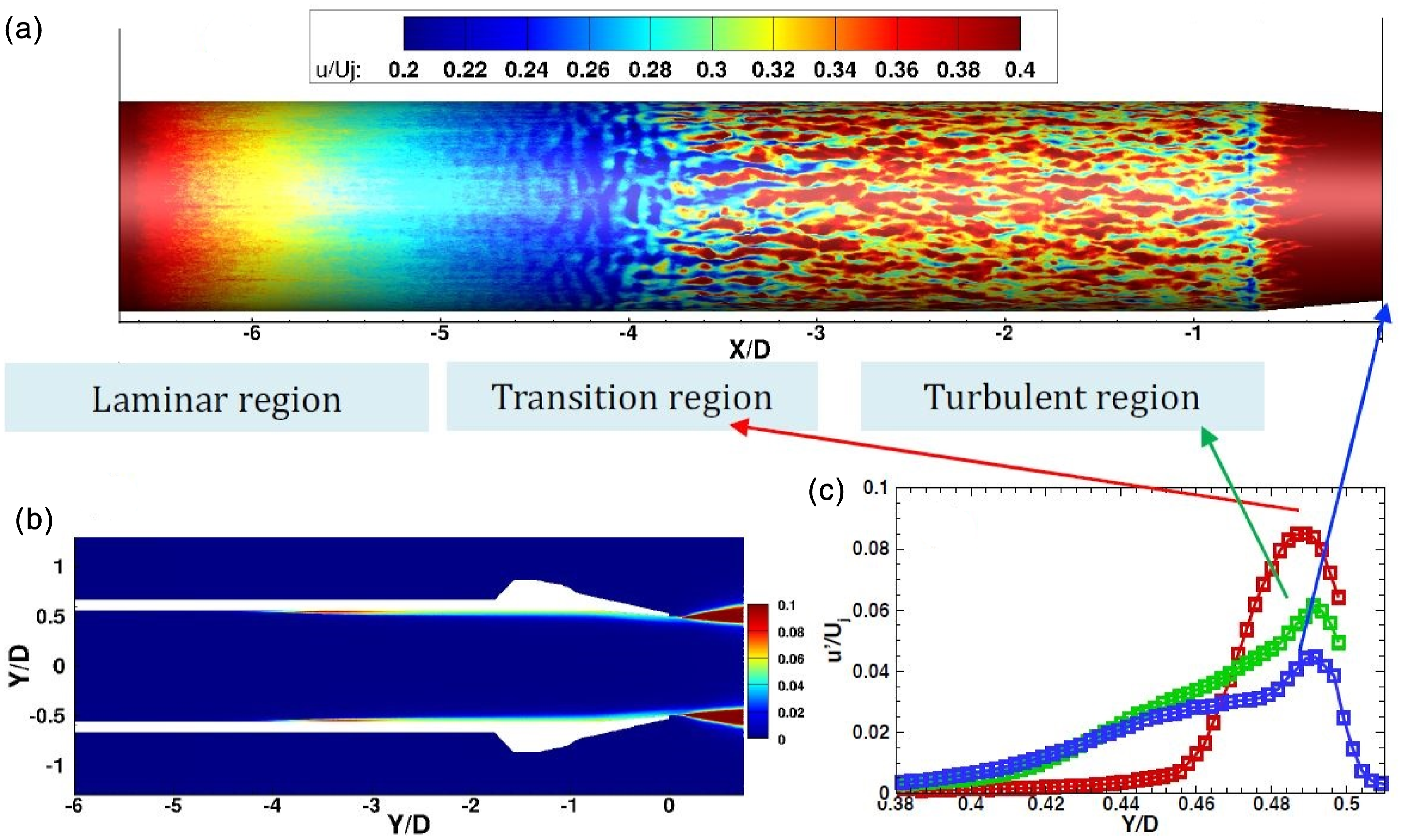

However, recall the earlier discussion of Figure 17. It appeared that the SMC nozzle BL went through transition, becoming highly disturbed laminar in the range 0.33< M_J < 0.55 and then turbulent around M_J = 0.6. Once turbulent it might be expected to remain turbulent with further increase in M_J. The mean velocity profile for the SMC case at M_J > 0.6, however, showed that it did not become turbulent. From M_J = 0.43 to 0.76 peak turbulence intensity decreased from 0.150 to 0.035 (Figures 18 and 19) but the mean velocity profile remained laminar-like. Thus, while the transition region in Figure 24(a) is expected to shift systematically with increasing M_J, for a contoured nozzle, different factors (e.g., compressibility, pressure gradient, tendency for BL separation in sections upstream, etc.) may act differently on the shift of the transition location. While it remains from being clear, such factors may have led to the counter-intuitive behavior of the BL state for the SMC nozzle at higher M_J.

Conclusions

Past research and current experimental results were used to examine the boundary layer states of high subsonic jets and their effect on radiated noise. Differences in subsonic jet noise databases from the literature were noted before. Noise data taken in ‘University-type’ facilities, involving higher contraction ratios and cleaner flows, were found to be of larger amplitudes relative to the data taken in ‘Industrial-type’ facilities. There was evidence that a difference in initial boundary layer state might be the root cause for the anomaly. Further experimental study was conducted with a set of 2-inch diameter nozzles, designed to vary the exit BL state, to investigate this. Nozzle exit BL profiles and the corresponding far field noise spectra and directivity were measured.

A variety of BL states were observed with the nozzles tested. A slow convergence near the exit yielded a turbulent BL that is relatively thick. A long cylindrical section at the end of the nozzle also yielded a turbulent BL. The shape factor (H₁₂) in such a BL is in the approximate range of 1.5–1.7. The peak turbulence intensity is low and around 5% of U_J. Such a low peak turbulence characterized all turbulent BLs in the present study. This contrasts the turbulent BL out of pipes or over flat-plates where much larger peak turbulence (10%–15%) have been reported in the literature. The difference is likely to be due to pressure gradients in the present nozzle flows.

With the ASME-type nozzles the BL is nominally-laminar. Here the BL is thin and its mean velocity profile is Blasius-like with a larger shape factor (H₁₂ ≈ 2). The peak turbulence intensity, however, vary over a large range. In some cases, the peak intensity is low (≈5%) and comparable to that of a turbulent BL. In other cases, it is high (≈15%), higher than even a flat-plate case. A laminar-like BL with high turbulence is denoted as highly disturbed laminar. It is remarkable that a state found with a given nozzle usually persisted throughout the Mach number range tested (up to M_J = 1). One nozzle (SMC) exhibited significant changes of the state with variation of M_J; the BL was highly disturbed laminar in the M_J range of 0.3–0.55 but the peak turbulence subsided while the profile remained thin and laminar-like at higher M_J.

It has been observed that simply a difference in BL thickness can cause a difference in radiated noise. Previous works such as those of Bogey & Marsden,³⁷ Brès et al.⁴¹ and Fontaine et al.⁴⁶ showed that with a thinner BL high-frequency instability waves grow more vigorously in the ensuing shear layer causing high turbulence and radiated noise. The noise difference due to thickness is seen regardless of BL state, i.e., for both laminar, both turbulent or one laminar and another turbulent case. As in the work of,⁴⁶ the present data show that the noise on the high-frequency end scales with the initial BL thickness. The thinner the BL the greater the noise. The present results furthermore illustrate that high initial turbulence cause additional increase in noise. Thus, a highly disturbed laminar BL, which is thin and also has high turbulence, is accompanied by the most significant increase in noise. Therefore, nozzles involving turbulent boundary layers are the quietest while nozzles involving a highly disturbed laminar state are the loudest especially on the high-frequency end of the spectrum.

Referring back to the discussion of the acceleration parameter in the Experimental Procedure section, we close with a comment about the BL states in the experiments of Tanna⁸ and Viswanathan⁷ that showed the difference in noise prompting this investigation. It is safe to infer that the BL was turbulent in.⁷ The nozzle geometry of⁸ involved a 45° conical contraction section reducing from 12” diameter to blend with a 2” diameter, short, cylindrical section at the end. The parameter K, calculated in a similar manner, turns out to be 3.84 at the end of the contracting section. This is a condition that would force the BL to become laminar. Thus, a laminar-like BL is quite expected at the nozzle exit. As stated before, the K criterion is only a rough guideline, and one cannot be certain about the BL state without experimental data. Nonetheless, from consideration of the K value as well as the noise characteristics it may be inferred that the jet exit BL in⁸ was most likely highly disturbed laminar.

Footnotes

Acknowledgements

The author is grateful to Dr James Bridges for help in various forms throughout the investigation, to Dr Cliff Brown for help with data acquisition in the AAPL, to Dr Amy Fagan for help with the schlieren data acquisition and to Dr Puja Upadhyay for miscellaneous help during the analysis of the results. In particular, the author likes to thank Dr Junhui Liu for the LES results. Comments on the preliminary manuscript by her and Drs James DeBonis, Stewart Leib and Nicholas Georgiadis are highly appreciated.

Declaration of conflicting interests

The author(s) declared no potential conflicts of interest with respect to the research, authorship, and/or publication of this article.

Funding

The author(s) disclosed receipt of the following financial support for the research, authorship, and/or publication of this article: This work was supported by the Transformational Tools and Technologies (TTT) and the Commercial Supersonics Technology (CST) Projects under NASA’s Aeronautics Research Mission Directorate.

ORCID iD

KBMQ Zaman

References

Zaman

KBMQ

. Increased jet noise due to a “nominally laminar” state of nozzle exit boundary layer. January, 2017. NASA/TM—2017-219440.

Zaman

KBMQ

. Exit boundary layer data for a round convergent nozzle in support of numerical simulation efforts. July, 2019. NASA/TM—2019-220242.

Liu

. Large-eddy simulations of nozzle-exit conditions in subsonic jet flows, Naval research laboratory. Washington, DC, 2020; vol. 191. Report NRL/MR/6041-20-10.

Zaman

KBMQ

. Effect of initial condition on subsonic jet noise. AIAA J 1985; 23(9): 1370–1373.

Zaman

KBMQ

. Effect of initial boundary-layer state on subsonic jet noise. AIAA J 2012; 50(8): 1784–1795.

Ahuja

. MPhil Thesis. London: London University, 1972.

Viswanathan

. Aeroacoustics of hot jets. J Fluid Mech 2004; 516: 39–82.

Tanna

. An experimental study of jet noise part I: turbulent mixing noise. J Sound Vib 1977; 50(3): 405–428.

Karon

Ahuja

. Validating the doubling-diameter method for rig noise detection in jet noise measurements. In: 23rd AIAA/CEAS aeroacoustics conference, Denver, Colorado, 5–9 June 2017, AIAA AVIATION forum.

10.

Lush

. Measurements of subsonic jet noise and comparison with theory. J Fluid Mech 1971; 46(3): 477–500.

11.

Olsen

Gutierrez

Dorsch

. The effect of nozzle inlet shape, lip thickness, and exit shape and size on subsonic jet noise. In: 11th AIAA aerospace sciences meeting, Washington, DC, 10-12 January 1973, AIAA-73-187.

12.

Harper-Bourne

. Commissioning and validation of a new jet rig for the QinetiQ noise test facility. In: 14th AIAA/CEAS aeroacoustics conference. Vancouver, BC, 5–7 May 2008, AIAA-2008-2958.

13.

Bridges

Brown

. Validation of the small hot jet acoustic rig for aeroacoustics research. In: 11th AIAA/CEAS aeroacoustics conference, Monterey, CA, 23–25 May 2005, AIAA-2005-2846.

14.

Harper-Bourne

. Jet noise measurements: past and present. Int J Aeroacoustics 2010; 9(4 and 5): 559–588.

15.

Viswanathan

Clark

. Effect of nozzle internal contour on jet aeroacoustics. Int J Aeroacoustics 2004; 3(2): 103–135.

16.

Schlichting

. Boundary layer theory. 7th ed. New York, NY: McGraw Hill Book Company, 1978.

17.

Bradshaw

. The effect of initial conditions on the development of a free shear layer. J Fluid Mech 1966; 26(No. 2): 225–236.

18.

Batt

. Layer some measurements on the effect of tripping the two-dimensional shear. AIAA J 1975; 13(No. 2): 245–247.

19.

Hill

Jenkins

Gilbert

. Effects of the initial boundary-layer state on turbulent jet mixing. AIAA J 1976; 14(11): 1513–1514.

20.

Hussain

AKMF

Zedan

. Effects of the initial condition on the axisymmetric free shear layer: effects of the initial momentum thickness. Phys Fluids 1978; 21(No. 7): 1100–1112.

21.

Hussain

AKMF

Zedan

. Effects of the initial condition on the axisymmetric free shear layer: effect of the initial fluctuation level. Phys Fluid 1978; 21(9): 1475–1481.

22.

Husain

Hussain

AKMF

. Axisymmetric mixing layer: influence of the initial and boundary conditions. AIAA J 1979; 17(1): 48–55.

23.

Raman

Zaman

KBMQ

Rice

. Initial turbulence effect on jet evolution with and without tonal excitation. Phys Fluid 1989; 1(No. 7): 1240–1248.

24.

Mollo-Christensen

. Jet noise and shear flow instability seen from an experimenter’s viewpoint. J Appl Mech 1967; 34: 1–7.

25.

Maestrello

McDAID

. Acoustic characteristics of a high-subsonic jet. AIAA J 1971; 9(6): 1058–1066.

26.

Grosche

F-R

. Distributions of sound source intensities in subsonic and supersonic jets. AGARD CP-131 1973; 4-1: 4–10.

27.

Bridges

Hussain

AKMF

. Roles of initial condition and vortex pairing in jet noise. J Sound Vib 1987; 117(No. 2): 289–311.

28.

Crighton

. Acoustics as a branch of fluid mechanics. J Fluid Mech 1981; 106: 261–298.

29.

Ahuja

. Correlation and prediction of jet noise. J Sound Vib 1973; 29: 155–168.

30.

Moore

. The role of shear-layer instability waves in jet exhaust noise. J Fluid Mech 1977; 80(No. 2): 321–367.

31.

Uzun

Hussaini

. Investigation of high frequency noise generation in the near-nozzle region of a jet using large eddy simulation. Theor Comput Fluid Dynam 2007; 21(4): 291–321.

32.

Bogey

Barré

Bailly

. Direct computation of the noise generated by subsonic jets originating from a straight pipe nozzle. Int J Aeroacoustics 2008; 7(1): 1–21.

33.

Bogey

Bailly

. Influence of nozzle-exit boundary-layer conditions on the flow and acoustic fields of initially laminar jets. J Fluid Mech 2010; 663: 507–538.

34.

Bogey

Marsden

Bailly

. Large-eddy simulation of the flow and acoustic fields of a Reynolds number 10⁵ subsonic jet with tripped exit boundary layers. Phys Fluids 2011; 23(No. 3): 1299–1312.

35.

Bogey

Marsden

Bailly

. Influence of initial turbulence level on the flow and sound fields of a subsonic jet at a diameter-based Reynolds number of 105. J Fluid Mech 2012; 701: 352–385.

36.

Bogey

Marsden

Bailly

. Effects of moderate Reynolds numbers on subsonic round jets with highly disturbed nozzle-exit boundary layers. Phys Fluids 2012; 24(No. 10): 1–24.

37.

Bogey

Marsden

. Identification of the effects of the nozzle-exit boundary-layer thickness and its corresponding Reynolds number in initially highly disturbed subsonic jets. Phys Fluids 2013; 25(No. 5): 1–27.

38.

Bogey

Marsden

. Simulations of initially highly disturbed jets with experiment-like exit boundary layers. AIAA J 2016; 54(No. 4): 1299–1312.

39.

Bogey

Sabatini

. Effects of nozzle-exit boundary-layer profile on the initial shear-layer instability, flow field and noise of subsonic jets. J Fluid Mech 2019; 876: 288–325.

40.

Bogey

. Generation of excess noise by jets with highly disturbed laminar boundary-layer profiles. AIAA J 2021; 59(No. 2): 569–579.

41.

Brès

Jordan

Jaunet

, et al. Importance of the nozzle-exit boundary-layer state in subsonic turbulent jets. J Fluid Mech 2018; 851: 83–124.

42.

Gryazev

Markesteijn

Karabasov

, et al. Flow and noise predictions of the isolated subsonic jets from the Doak laboratory experiment. In: 28th AIAA/CEAS aeroacoustics conference, Southampton, 14–17, AIAA Paper 2022-2935.

43.

Karon

Ahuja

. Effect of nozzle-exit boundary layer on jet noise. In: 51st AIAA aerospace sciences meeting, Grapevine, Texas, 7–10 January 2013, AIAA Paper 2013-0615.

44.

Karon

Ahuja

. Reynolds number and the jet noise scaling relationships. In: 23rd AIAA/CEAS aeroacoustics conference, Denver, CO, 5-9 June 2017, AIAA. paper 2017-3861.

45.

Karon

Ahuja

. Role of nozzle-exit boundary layer in producing jet noise. Int J Aeroacoustics 2022; 21(Issue 5–7): 626–653.

46.

Fontaine

Elliott

Austin

, et al. Very near-nozzle shear-layer turbulence and jet noise. J Fluid Mech 2015; 770: 27–51.

47.

Murray

Lyons

Thurow

, et al. A laboratory framework for synchronous near/far-field acoustics and MHz PIV in high-temperature, shock-containing, jets. In: Proceedings of the internoise 2012/ASME NCAD meeting, New York City, NY, 19–22 August 2012, NCAD2012, ASME/NCAD-1270.

48.

Narasimha

Sreenivasan

. Relaminarization of fluid flows. Adv Appl Mech 1979; 19: 221–309.

49.

Fagan

L’Esperance

Zaman

KBMQ.

Application of a novel projection focusing Schlieren system in NASA test facilities. In: 30th AIAA aerodynamic measurement technology and ground testing conference, Atlanta, GA, 16-20 June 2014, AIAA Paper 2014-2522.

50.

Brown

. Jet-surface interaction test: far-field noise results. In: Proceedings of the ASME turbo expo 2012, Copenhagen, Denmark, 11-15 June 2012.

51.

Liu

Corrigan

Johnson

, et al. Effect of nozzle inflow conditions on shock-cell structure and noise in overexpanded jets. In: 25th AIAA/CEAS aeroacoustics conference, Delft, Netherlands, 20 May 2019, AIAA Paper 2019-2495.

52.

Stitch

Housman

Kocheemoolayil

, et al. Large-eddy simulation of jet surface interaction noise. In: 25th AIAA/CEAS aeroacoustics conference, Delft, Netherlands, 20 May 2019, AIAA Paper 2019-2475.

53.

Khavaran

Kenzakowski

. Progress toward improving jet noise predictions in hot jets, 2007. NASA/CR—2007-214671.

54.

Uzun

Hussaini

. Prediction of noise generated by a round nozzle jet flow using computational aeroacoustics. J Comput Acoust 2011; 19(03): 291–316.