On the application of matching pursuit decomposition to jet noise data

Abstract

The Matching Pursuit decomposition is a signal processing technique that projects a signal onto a linear expansion of waveforms selected from a redundant set of arbitrary functions, collectively referred to as a Dictionary. A key feature of this method is its ability to reconstruct a signal using a carefully chosen subset of these waveforms. In the present paper, this method is applied to illustrate its potentialities for reduced-order modeling of jet noise data. The analysis is conducted on an experimental dataset containing pressure time series taken in both the near- and far-field of a compressible subsonic free jet. For this application, the Dictionary is constructed using Gabor functions, and it is shown that even with a very limited number of atoms (one thousand), significant physical properties of the near pressure field are preserved. The results demonstrate that the effects of Mach number, as well as radial and axial distances from the jet exit, are accurately reproduced in both spectral features and temporal correlations. In the frequency domain, the energy bump at the Kelvin-Helmholtz frequency is effectively captured, primarily in the region close to the jet exit. Additionally, the non-zero correlations between near- and far-field pressure fluctuations are correctly captured, along with the corresponding phase lag obtained from the correlation maxima. The analysis confirms that the Matching Pursuit decomposition adaptively selects atoms that best represent the original signals. The superposition of a limited number of these optimally chosen atoms provides a highly simplified yet physically meaningful representation of the complex original signals. Future developments and applications aimed at modeling jet noise sources and predicting acoustic radiation are also outlined.

Keywords

time-frequency decomposition matching pursuit jet noise reduced order modelling experiments

Introduction

Aeroacoustic signals are inherently unsteady and often characterized by time-localized events and time-varying frequency content. This is due to the non-deterministic nature of the acoustic field that in numerous configurations, like jets and wakes, is generated by noise sources localized in regions where the flow is turbulent.¹ Efficient processing of these signals necessitates the use of Time-Frequency (TF) decomposition techniques that can overcome the limitations of standard Fourier analysis that is not well-suited for extracting time-localized features.

TF decomposition techniques have been developed and applied in various fields, including biomedicine, communication, speech, earthquake analysis, turbulence, and vibrations. It is known (see e.g.²) that the most direct way to provide a TF analysis using standard methodologies is to adapt the FFT procedure by proper signal windowing. This is the so-called Short-Time Fourier Transform (STFT) that is based on the idea of splitting a given signal into small time windows through a proper windowing and then applying the FFT to each time segment or block. STFT has been used in aeroacoustic applications to analyse both broadband and tonal noise components characterized by time varying acoustic power at different frequencies (e.g.^3,4,5). The result of the STFT is a two-dimensional time-frequency representation with a constant bandwidth or resolution, regardless of the actual frequency. This is the main limitation of this approach where the accuracy of obtaining frequency information is limited by the length of the window according to the duration of the block.

This shortcoming can be overcome by using the Wavelet Transform (WT), which employs localized functions to capture both frequency and temporal information across various scales. This technique is particularly effective for analyzing transient or unsteady signals, as it offers improved resolution for signals undergoing abrupt changes. The Wavelet transform accomplishes the need to overcome the limitations of the STFT by increasing the resolution at small scales. For this purpose, the base of functions is generated by the dilation and translation of a unique compact-support function named the Mother Wavelet, that is chosen appropriately. Both single and multivariate Wavelets have been extensively used in turbulence and aeroacoustics, primarily to highlight features associated with intermittency and to establish causality-based procedures for identifying noise sources (see among many^6,7,8). It is important to emphasize that the way the Wavelet basis of functions is derived from the Mother Wavelet represents the major limitation in the Wavelet Transform, as the central frequency of the spectral bandwidth of the analyzing function is constrained to be inversely proportional to the scale. Specifically, the shape of the Mother Wavelet is maintained across all scales, with its width adjusted based on the desired resolution, while the number of oscillations remains fixed.

A methodology that may overcome this further limitation is the Matching Pursuit (MP) decomposition, a method that decomposes a signal into a linear combination of waveforms taken from a predefined set of functions called Dictionary. This technique is highly flexible and enables the representation of complex signals with varying characteristics, providing a sparse representation that captures essential features of the original signal. The MP selects a best basis, not necessarily orthogonal, that efficiently approximates the signal of interest overcoming the limitations of both the STFT and the WT. As will be demonstrated below, the method increases the number of parameters available, providing an over-complete Dictionary that includes a broader range of time and frequency support functions. This allows for instance to represent efficiently signals that are extended in time but narrow in frequency, or vice versa, situations that cannot be effectively managed by either the STFT or the WT.

The method, introduced by Mallat & Zhang,⁹ has been applied for the analysis of temporal signals or images in several fields (see among many,^10,11,12,13). In the framework of aeroacoustics, the MP application has been limited to implementations in the context of acoustic Beamforming (^14,15) and for the estimation of Green functions in complex configurations.¹⁶

In the present work, the MP technique is applied for the first time to jet noise data, and its potentialities for reduced-order modelling are demonstrated.

The main features of the method, including a description of the algorithm adopted for its numerical implementation, are given in the following Section. The dataset analyzed consists of pressure signals measured in a jet noise experiment. The setup is briefly described in what follows along with the flow conditions and the acquisition parameters. The remaining sections contain the main results and the conclusions including a brief discussion about possible future applications in aeroacoustics.

The matching pursuit decomposition

The MP Decomposition provides an optimal non-linear approximation of a signal by adaptively choosing the proper basis depending on the signal nature. The basic idea is to construct an optimal basis, not necessarily orthogonal, that efficiently approximates the signal of interest. The MP algorithm iteratively constructs an approximation by selecting a set of elementary waveforms, called atoms, chosen from an over-complete set of functions, called Dictionary, such that they represent at the best the inherent signal features.

A crucial part of MP is the creation of the Dictionary which directly affects the results of the decomposition and subsequently the quality of the signal reconstruction. To the purpose of the time-frequency decomposition, the waveforms belonging to the Dictionary are usually selected as time-frequency atoms obtained as dilations, translations, and modulations of a single window function. According to the formalism introduced by,⁹ the window function in the temporal domain t can be denoted as follows:

g_{γ} (t) = \frac{1}{\sqrt{s}} g (\frac{t - u}{s}) e^{i ξ t}

(1)

Where γ is the index that represents the set of parameters (s, u, ξ) of the element selected within the Dictionary, and

\frac{1}{\sqrt{s}}

is a normalizing factor. More specifically, u and s give the translation and dilation factors, respectively, and ξ is the frequency.

The family of g(t) functions is generated by varying the three parameters (s, u, ξ) independently from each other. In this way, the Dictionary is extremely redundant and contains many functions that can be selected appropriately to provide the best approximation. As pointed out in the previous section, this method results to be more flexible than the STFT and WT. STFT corresponds to fixing the scale s to a certain value, whereas in the WT, the frequency parameter ξ is forced to be inversely proportional to the scale s.¹⁷ have shown that MP is better suited even with respect to Wavelet Packets for non-stationary signals. Wavelet packets correspond to precise frequency ranges that are directly connected with the selection tree of the algorithm whereas in the MP approach the choice of the atoms is completely free.

To the purpose of the present application, the Dictionary is composed of Gabor atoms that provide optimal joint time–frequency localization. The Gabor Dictionary contains functions obtained by the combination of a Gaussian envelope of variable time location and extension, with a cosine function of variable frequency.

The Gabor waveform can be formalized as follows:

g_{γ} (t) = K_{γ} (t) {\cdot G}_{γ} (t) = K_{γ} (t) \cdot \exp [- π {(\frac{t - u}{s})}^{2}] \cos (2 π ξ t + φ)

(2)

where the factor

K_{γ} (t)

represents the energy content of the atom i.e.:

K_{γ} (t) = {(\int_{- \infty}^{\infty} {G_{γ} (t)}^{2} d t)}^{- 1 / 2}

(3)

The Dictionary is thus composed of a set of Gabor functions having three variable parameters (s, u, ξ). The selection of the functions best matching the given signal is accomplished through an iterative computation of a correlation function. This is the core of the procedure used in the numerical implementation of the MP algorithm. The details can be found in the literature (e.g.^9,10) but the main features are briefly worked out in what follows.

The MP procedure is based on an iterative process that maximizes the correlation between the signal reconstructed through the combination of the atoms belonging to the Dictionary and the original signal. Denoting with x the analyzed signal, the algorithm iteratively selects the atoms that provide the best approximation of x. The iterative process starts with the selection of the atom within the Dictionary that best describes the whole signal and its projection onto the signal is subtracted from it to achieve a residual. In other words, at the first step the Dictionary is scanned to search for the atom $g_{γ, 1}$ for which the correlation or inner product $| 〈 {x, g}_{γ, 1} 〉 |$ is as large as possible. The residual $R^{1} x$ at the first step is obtained by the following relationship:

x = | 〈 {x, g}_{γ, 1} 〉 | + R^{1} x

(4)

At the successive step, the atom

g_{γ, 2}

is identified by finding the maximum correlation with

R^{1} x .

The procedure is then repeated iteratively with the residual replacing the signal.

The algorithm can then be formalized by the following three steps:

{\begin{cases} R^{0} x = x \\ R^{i} x = 〈 R^{i} {x, g}_{γ, i} 〉 g_{γ, i} + R^{i + 1} x \\ g_{γ, i} = \arg \max_{g_{γ, i^{'}} \in D} 〈 R^{i} {x, g}_{γ, i^{'}} 〉 \end{cases}

(5)

In other words, at each iteration, the MP algorithm looks for the atom which is the most strongly correlated with the signal x , i.e., which has the highest absolute inner product with the signal. The steps of the algorithm can be summarized as follows:

(1) Initialization: for ${i = 0, x}_{i} = x_{0} = x$ , which means that at the first step, the entire original signal $x$ is considered

(2) Computation of the correlations between the signal $x_{i}$ and every atom in the Dictionary, using inner products

(3) Search for the most correlated atom ${\hat{g}}_{i}$ by searching for the maximum inner product

(4) Computation of the weight $w_{i} = 〈 x_{i}, {\hat{g}}_{i} 〉$

(5) Computation of a residual that represents a new version of the signal: $x_{i + 1} = x_{i} - w_{i} {\hat{g}}_{i}$

(6) Stop of the iterations whether the desired level of accuracy is reached or re-iteration of the pursuit (i.e. go to step 2) using the residual as input file.

Thus, the standard MP algorithm starts with an initial approximation that is empty and a residual that equals the original signal. At each iteration it subtracts from the residual the atom that has the highest correlation with it and adds that atom to the approximation. Continuing in this procedure, MP builds-up the signal model one atom at a time and at each iteration. The MP algorithm iteratively selects the atom that best correlates with the current residual, reducing the residual at each step and thus guarantees that the residual norm decreases monotonically, ensuring convergence in the sense that the residual energy diminishes over iterations. In this regard,¹⁸ showed that the residual goes to zero when the number of iterations goes to infinity. In practice, iterations are stopped when the desired level of accuracy is reached in terms of the number of extracted atoms or, as in the present case, in terms of the energy ratio between the original signal and the current approximation.

We note that the speed at which MP converges toward the original signal is influenced by how well the Dictionary atoms can represent the signal features. A highly redundant or overcomplete Dictionary may have slow convergence but can provide a sparser and more accurate representation. Therefore, while the MP algorithm guarantees a decreasing residual energy, the rate of convergence varies depending on the problem specifics. Theoretically, it converges asymptotically, but, in practice, convergence speed and accuracy depend heavily on the Dictionary properties and the chosen stopping conditions.

We note that the non-orthogonality of the basis employed in the MP procedure results in a non-unique signal representation, resulting in the set of functions in the Dictionary to be overcomplete. This means that there can be multiple, redundant atoms beyond the minimum necessary, providing alternative ways to approximate the same signal. As noted in⁹ and,¹⁹ non-uniqueness offers the advantage of adaptability. It enables selecting, from many possible representations, the one most suited to the analysis objectives. This approach ensures the sparsest possible representation of the signal, using the fewest atoms. Furthermore, the non-uniqueness grants flexibility to choose basis functions arbitrarily according to the signal nature. For a given number of atoms, different basis selections can produce reconstructions with different accuracy. For instance, a signal dominated by tonal components is best reconstructed using a Dictionary of trigonometric functions. Alternatively, frequency-localized Gabor functions can be used for reconstruction, but obtaining a good approximation generally requires a significantly larger number of atoms compared to Fourier waveforms. We refer to the literature for further details about convergence⁹ and possible variants of the MP procedure (see e.g.^20,21,13). In the present analysis, the MP algorithm is applied in the Matlab framework, using the tool developed for processing 1D signals²². To the extent of the computational demand of using this method, we note that increasing the number of atoms results in a greater number of iterations in the algorithm and thus longer CPU time. Additionally, the longer the signal (in our case, 4 × 10^6 samples), the longer the CPU time. This means that analyzing very long signals consisting of millions of samples and projecting over thousands of atoms, could entail significant computational effort, potentially requiring hours of processing time on a standard commercial PC.

Experimental set-up and flow conditions

The pressure dataset refers to experiments performed in the anechoic chamber of the Laboratory of Fluid Dynamics “G. Guj” of Università Roma Tre of Rome. The investigation has been carried out to characterize the aeroacoustics of a single stream cold jet, having an exit diameter D of 0.012 m. Near-field pressure measurements have been carried out at three radial distances, that is, r/D=1, r/D = 2, and r/D=3, with reference to the position of the microphones at x/D=0, along straight lines inclined of 10° with respect to the jet axis in order to follow the jet spreading. Different axial positions spanning from 1D to 20D downstream are considered at Mach numbers 0.7 and 0.9. Measurements in the near-field have been carried out using one microphone installed close to the jet axis on a wooden support and moved using a manual micrometric traversing system. The far-field pressure signal is acquired simultaneously with those from the near-field transducer using a microphone installed at a distance of about 70D from the jet exit at a polar angle of 30° with respect to the jet axis, which corresponds to the region of maximum jet-noise directivity. A scheme of the setup is given in Figure 1.

Figure 1.

Scheme of the jet noise experiment (the scales and proportions are not preserved). The x-axis is aligned with the mean velocity. s denotes the distance between a generic near-field microphone and the far field microphone whereas h is the distance between the far field microphone and the jet exit. Note that the near-field microphones were aligned with the jet shear layer with an inclination angle of 10°.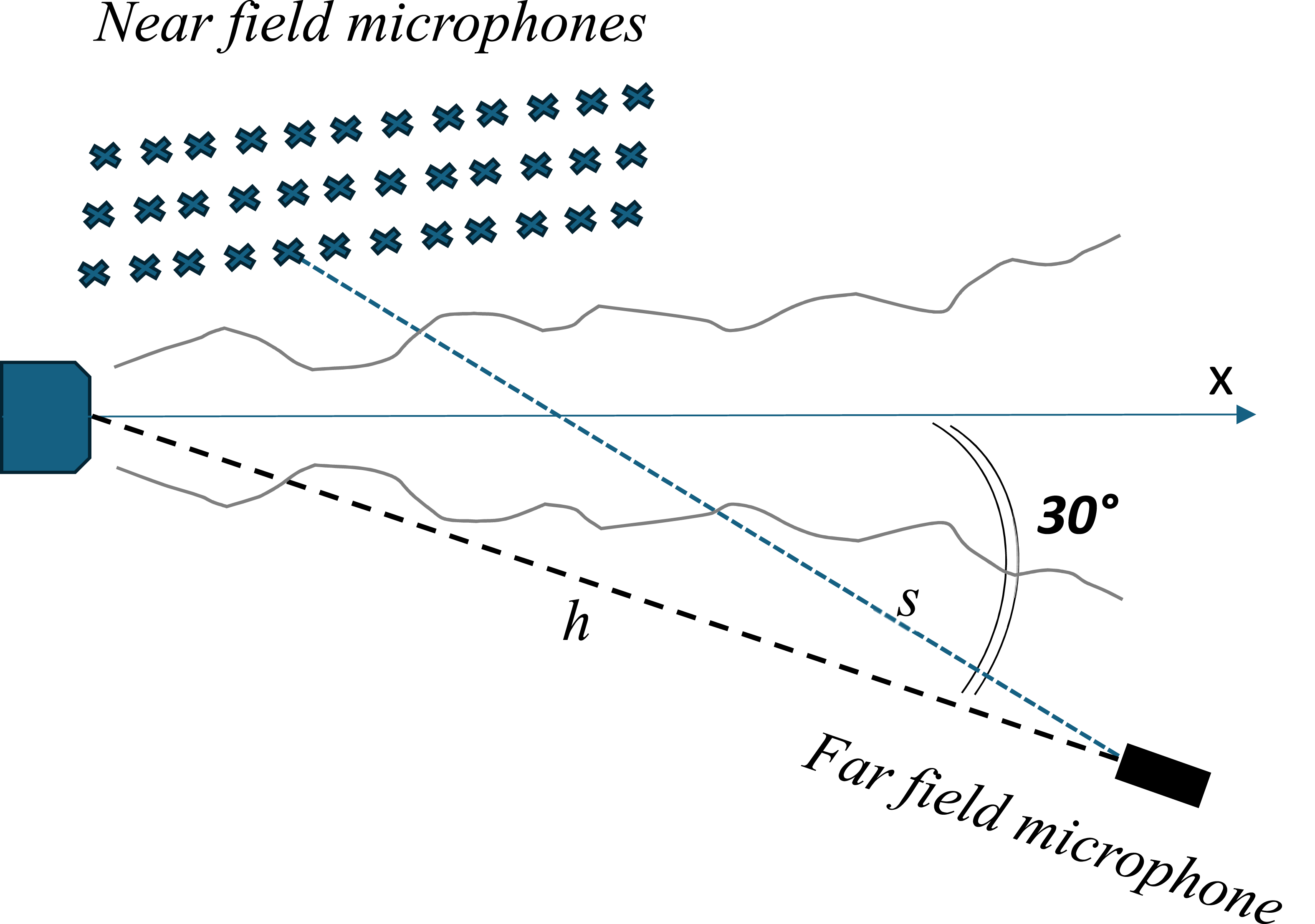

Both the near- and far-field microphones were 1/4” 4135 Bruel & Kjaer type and they were both calibrated using a B&K 4228 Pistonphone generating a sound pressure level (SPL) of 94 and 114 dB at 1 kHz. The microphones were installed without the protecting grid so as to have, according to the calibration charts, a flat frequency response up to approximately 100 kHz. The microphones were connected to a B&K Nexus 2690 multi-channel signal conditioner that allows for setting the amplification gain and the analog anti-aliasing filter. The signals were acquired through a Yokogawa Digital Scope DL708 E setting the sampling frequency to 500 kHz and the number of acquired samples per each position to 4x10⁶. The facility as well as the jet geometry and the test chamber, are described in detail in ref. 23 and 24.

Results

Before going into detail of MP-based re-construction of the near-field pressure content, an overview of the temporal and spectral properties of the atoms composing the Dictionary is provided along with the criteria adopted for selecting the amplitude and range of variation of the parameters characterizing the atoms. Figure 2 reports examples of Gabor atoms belonging to the Dictionary that have been adopted for the present investigation. The waveforms depicted in Figure 2 represent two samples characterized by a different frequency ξ (see equation (2)) taken from the complete set of available atoms. Specifically, case (a) corresponds to the Gabor function having the minimum ξ among the atoms of the Dictionary. It corresponds to a Strouhal number (St), based on the mean velocity and the jet diameter, of about 0.01, thus much lower than the minimum St of interest for jet noise. The Gabor waveform with maximum ξ is instead reported in Figure 2(b). It corresponds to St of about 3, in this case much larger than the maximum St of interest for the jet noise analysis.

Figure 2.

Examples of atoms taken from the Dictionary. (a) Atom with lowest frequency; (b) Atom with the highest frequency.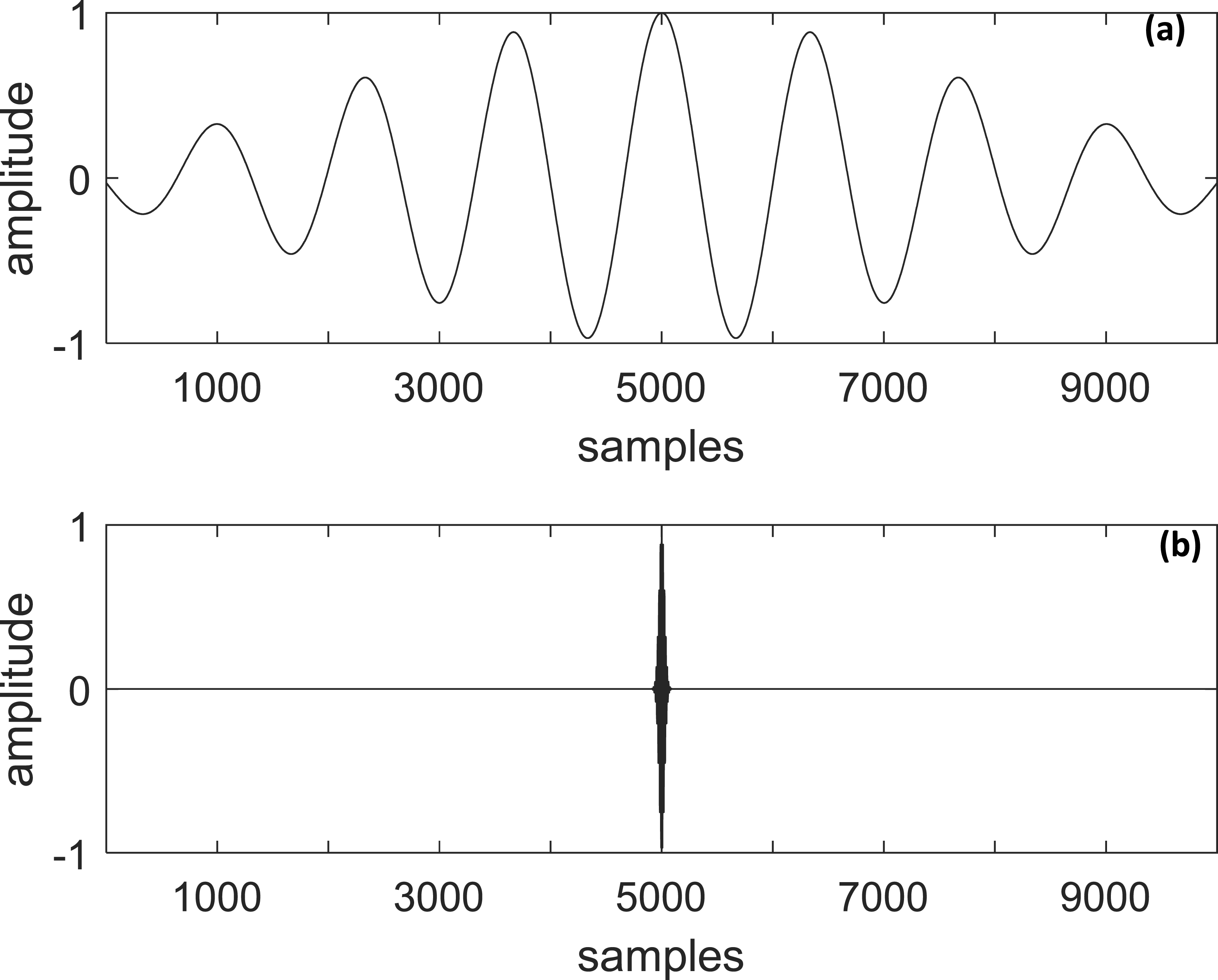

Figure 3 shows the Power Spectral Densities in dB (the Sound Pressure Level - SPL) of a few Gabor atoms within the frequency range selected for the present analysis. We note that each single atom has a narrowband frequency content and that the set of selected waveforms span the whole range of frequencies of interest for the present application.

Figure 3.

Auto-spectra of atoms having different frequencies (different colors correspond to atoms of different frequencies).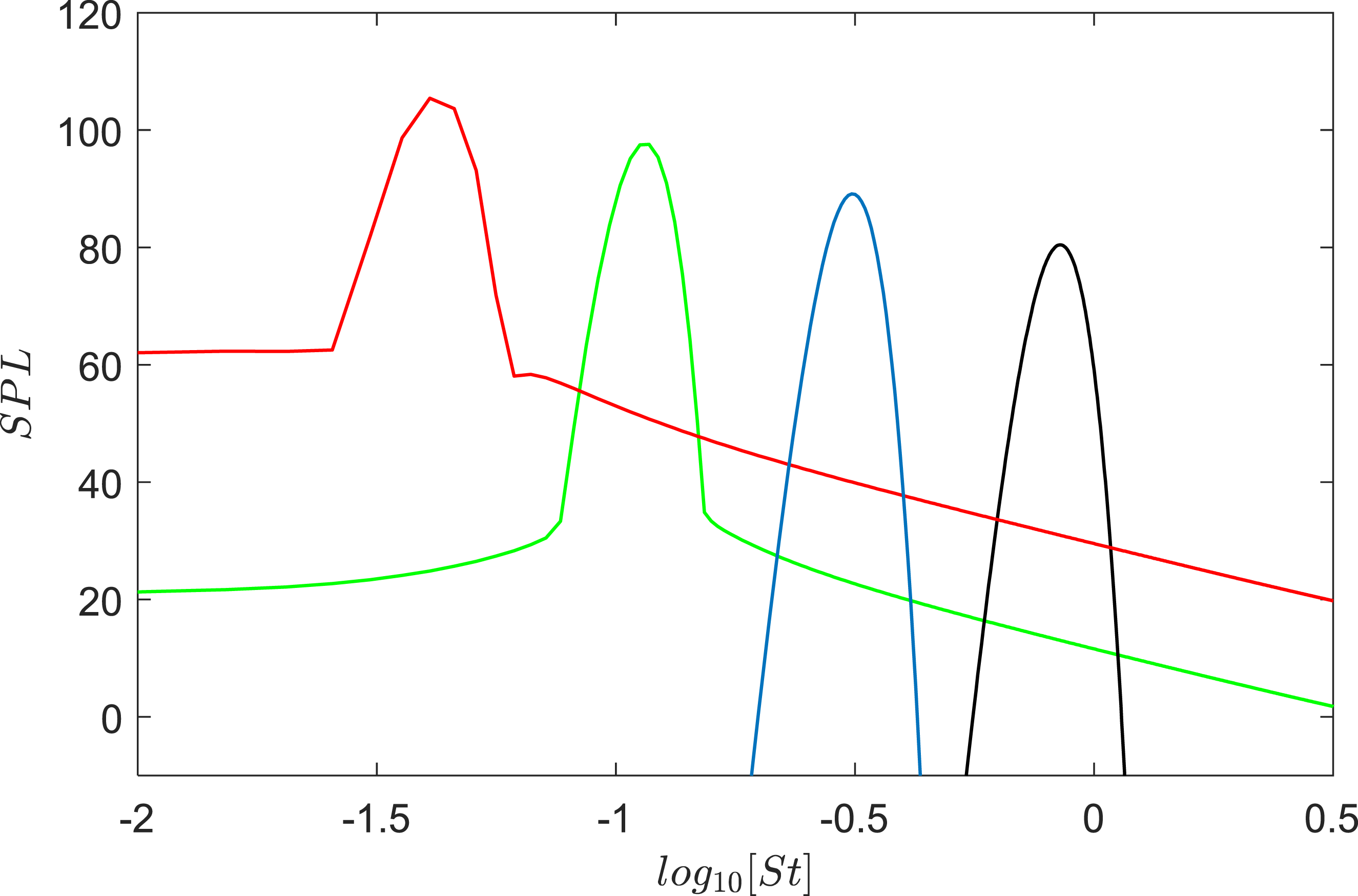

With reference to equation (2), the parameter $u$ indicates the temporal position of the atoms and varies within an interval corresponding to the duration of the analyzed signal. The parameter $s$ corresponds to the lifetime of the Gaussian envelope. Its maximum amplitude is set based on the typical time-scale of the largest flow structures relevant to aerodynamic and aeroacoustic behavior, and, when converted to space using the mean flow velocity, it corresponds to about 10 diameters.

Depending on the properties of the signal to analyze, the MP iterative algorithm adaptively selects those atoms that are able to reproduce correctly spectral features of the original signals, and the combination of several atoms provides modelling of broadband spectral features. Indeed, as pointed out above, by increasing the number of atoms, the similarity between the reconstructed signal and the original one improves. An example illustrating this aspect in the spectral domain is given in Figure 4. The auto-spectra of signals reconstructed using different numbers of atoms are reported and compared to the spectrum of the original signal. It is clearly shown that the higher the number of atoms the closer the reconstructed spectrum is to the original one. As indicated in,⁹ when the number of atoms tends to infinity, the signal is reconstructed perfectly, and the residual is zero. However, even with the minimal number of atoms, as in the case of 100 atoms of Figure 4(a), the MP algorithm adaptively selects those atoms whose frequency content effectively reproduces the most energetic range of the original signal. Figure 4(b) reports the ratio between the variance of the reconstructed signal and that of the original one (denoted as energy ratio) as a function of the number of atoms adopted in the reconstruction. It is clear that the curve increases monotonically and that a 100% energy ratio (perfect reconstruction) is reached for an infinite number of atoms. Similar results are obtained for the other configurations presently analyzed.

Figure 4.

Effect of the number of atoms determined for the case M=0.9, x/D=4 and r/D=1. (a) Spectral content of signals reconstructed using different numbers of atoms compared with the original SPL. (b) Energy ratio in percentage, as a function of the number of atoms.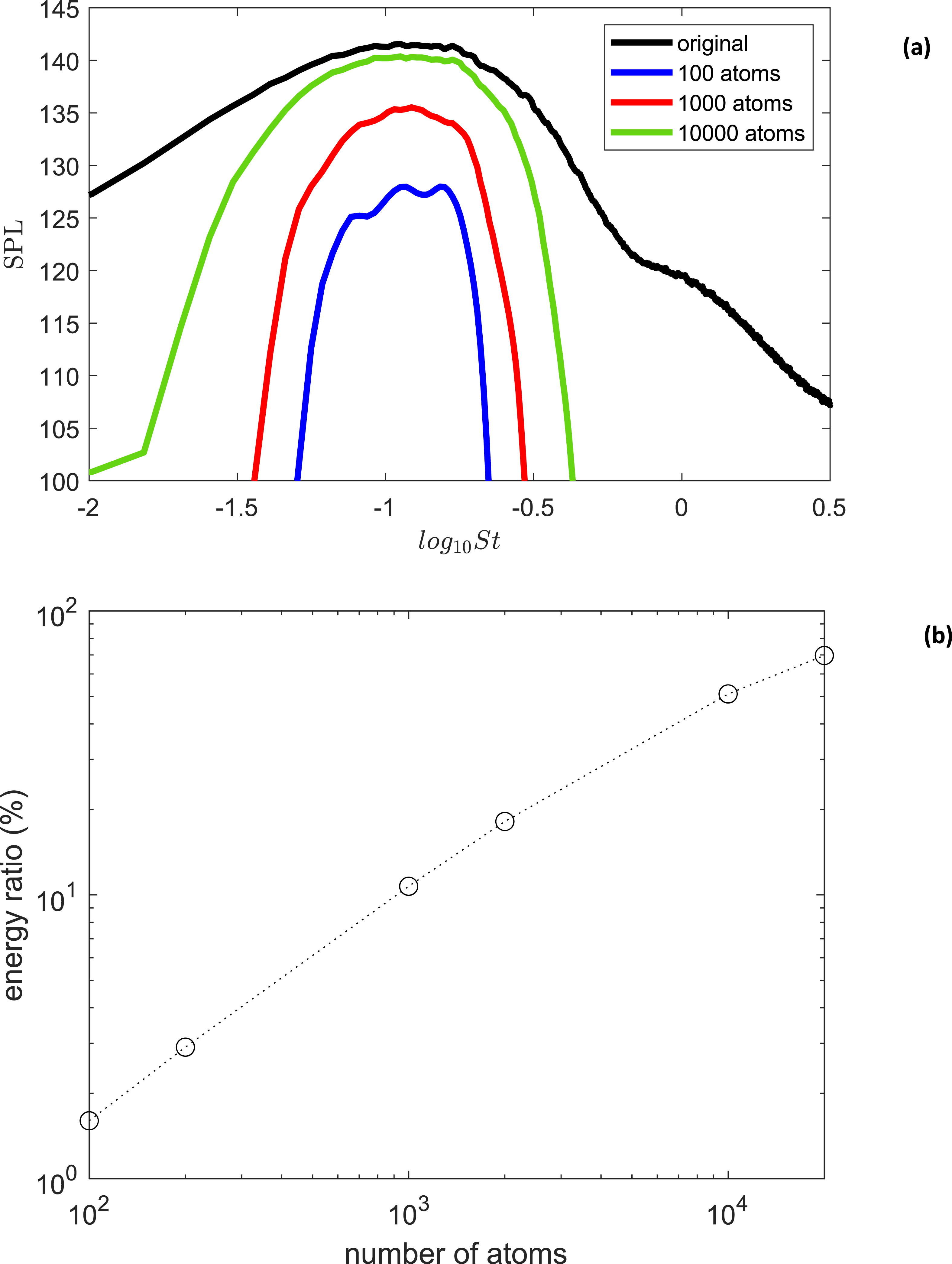

To the purpose of providing a reduced order modeling of the measured pressure signals, in the present analysis the reconstruction is accomplished using 1000 atoms. The criterion adopted to fix this number of atoms is based on the energy contained by the reconstructed signals. As shown in Figure 4(a), using 1000 atoms the energy of the reconstructed signals is one order of magnitude lower (i.e. of the order of 10%) than that of the original ones. The aim of the present investigation is indeed to demonstrate that a signal reconstructed via the MP procedure, containing energy that is an order of magnitude smaller than that of the original one, still preserves the key physical properties of the original signal.

An example of a reconstructed signal as a function of time is provided in Figure 5 along with the original signal. It is shown that the reconstructed signal consists of a few selected atoms randomly distributed in time (thus with a random phase), having different frequencies and amplitudes. The phase of the atoms corresponds to the choice of the parameter u in equations (1) and (2) that is adaptively selected by the algorithm in the iterative process and thus it represents an output of the processing. This means that there is no a-priori forcing on the phase (and of its statistical properties). This reasoning is valid also for the frequency and amplitude of the selected atoms that are not predetermined but rather derived as outputs of the MP algorithm. We remind the reader that the reconstructed signal is much simpler compared to the random, complex, and unpredictable measured time series.

Figure 5.

Example of a segment of a reconstructed signal using 1000 atoms (blue line). The red line is the original signal. The time axis corresponds to the inverse of the Strouhal number, that is 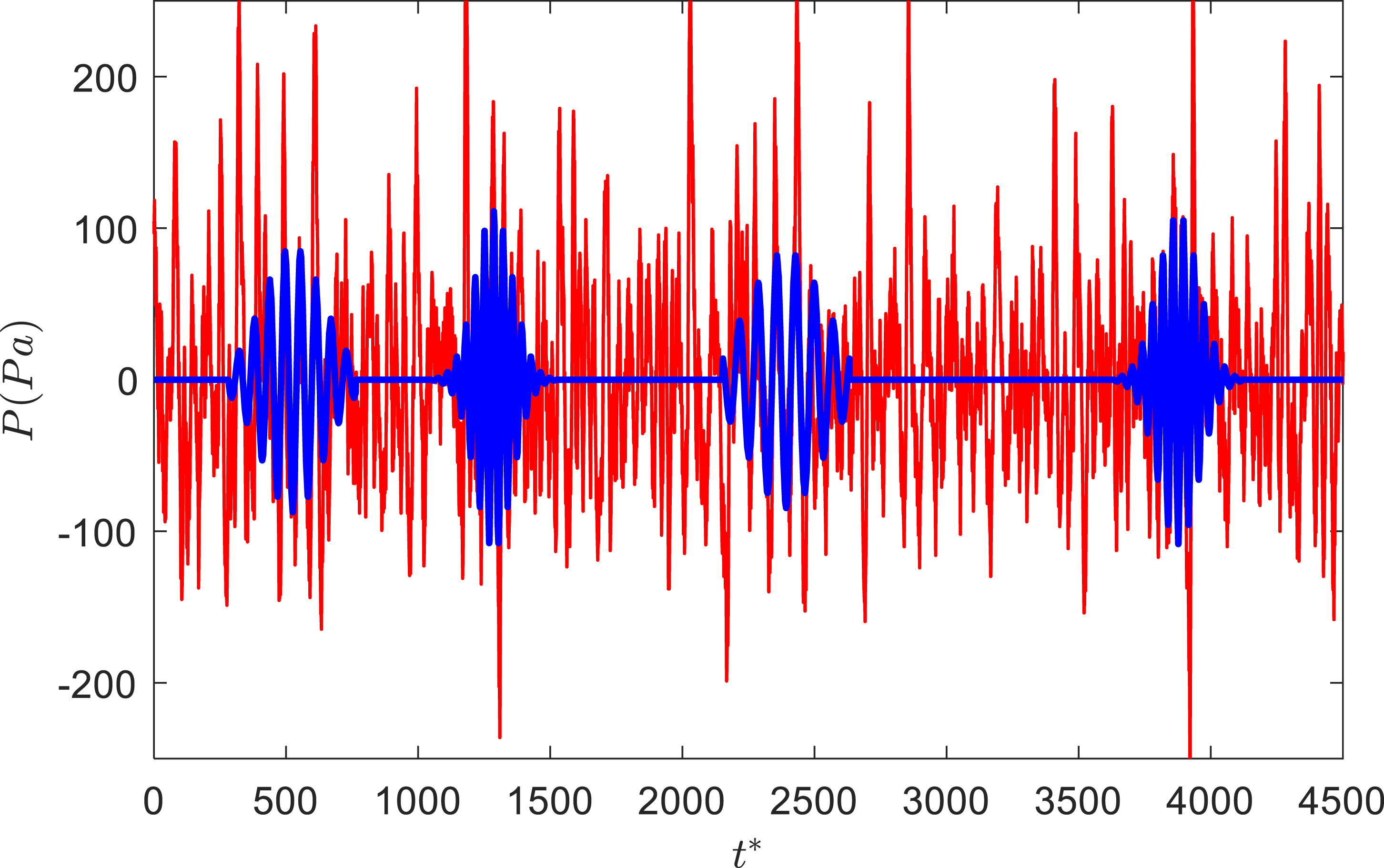$t^{*} = \frac{t U}{D}$ .

The number of atoms selected is very low and thus, as shown in Figure 4(a), the frequency distribution of the spectral energy is not broadband. However, depending on the nature of the analyzed signal, the algorithm is able to select adaptively those atoms that match as best as possible the original spectral content. The examples reported in Figure 6 highlight this property. The reported spectra are taken close to the jet exit for M=0.9 and r/D=1.Case (a) corresponds to x/D=1 and the signal exhibits a relevant tonal contribution, highlighted by the black arrow, at a frequency that corresponds to the Kelvin-Helmholtz mode. The algorithm is able to reproduce this effect that is dominant with respect to the other spectral components. In this case, the spectrum of the reconstructed signal is almost tonal, and this implies that the 1000 atoms used for the reconstruction have almost the same frequency. In case (b), taken at x/D=3, the tonal component of the original spectrum is less prominent with respect to the broadband one, and in the reconstruction procedure, the weight of the broadband contribution becomes more significant. In this case, the frequency of the atoms is more variable. Case (c) reports the case at x/D=6 and a fully broadband spectrum is observed. In this condition, the tonal contribution is no longer visible in the original spectrum as well as in the reconstructed one. In the present dataset, depending on the flow configuration, corresponding to a certain distance from the jet axis, radial position, and Mach number, all the three situations reported in Figure 6 may occur and the capability of the method to adapt the frequency content of the reconstructed signal to that of the analyzed one has been verified in all cases.

Figure 6.

Example of the auto-spectra of signals reconstructed using 1000 atoms (blue bold line) compared to the spectra of original signals (black line). (a) Signal containing a tonal component, indicated by the black arrow (pressure signal taken close to the jet exit); (b) Signal containing both tonal and broadband components (pressure signal taken close to the end of the jet potential core); (c) Signal containing only broadband components (pressure signal taken downstream the end of the potential core).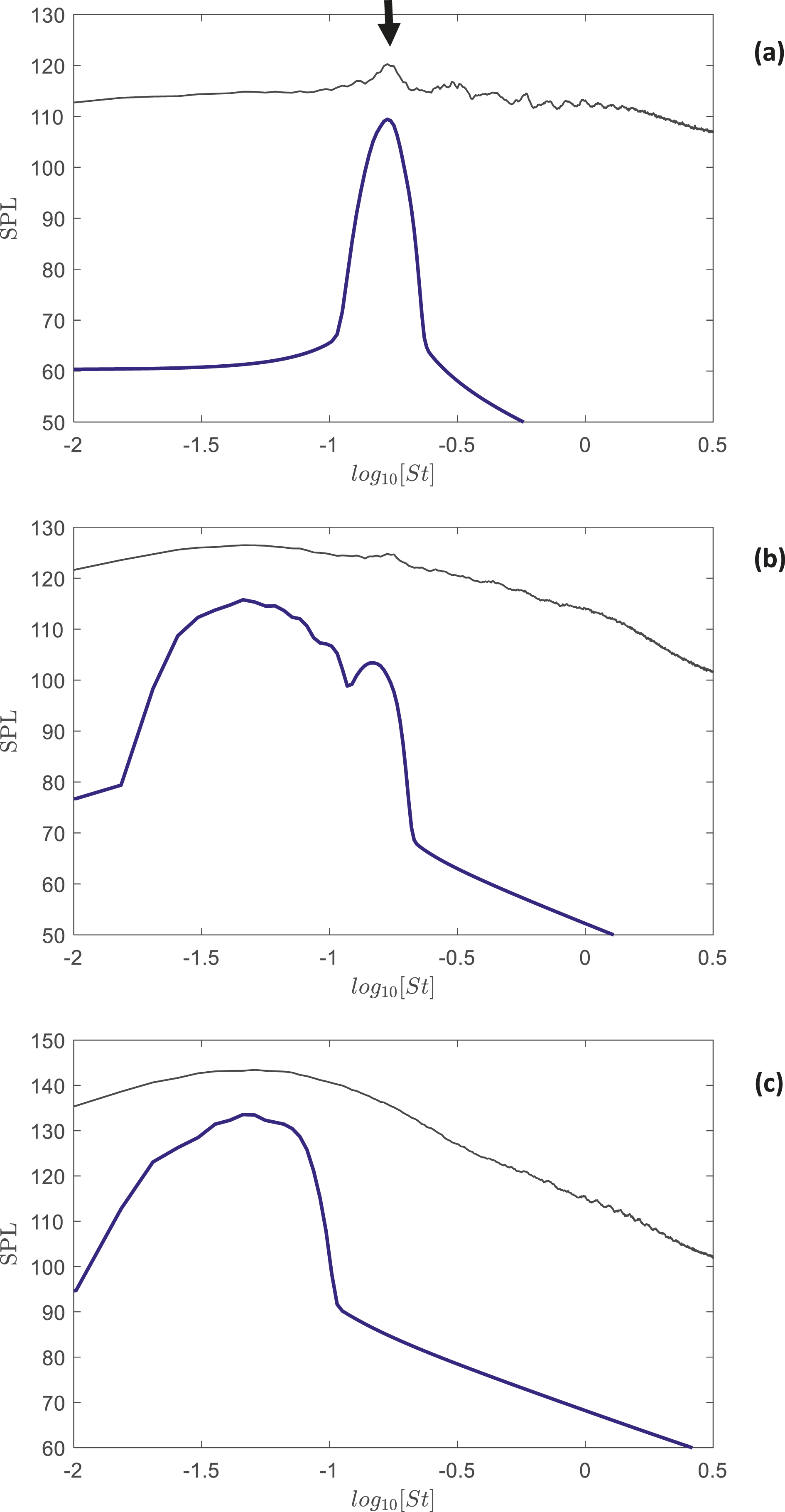

In addition to the differing contributions of tonal and broadband components in the power spectra, the energy-containing amplitude and frequency range may also vary significantly depending on the analyzed conditions. According to the literature,²⁴ the spectral bump related to the hydrodynamic pressure in the near-field is expected to increase in intensity for increasing x/D but the frequency range corresponding to the maximum energy is expected to move towards lower frequencies. The spectral energy is also expected to decrease for increasing radial distances from the jet axis because of the expected exponential decay with r/D of the hydrodynamic pressure (see e.g.²⁵).

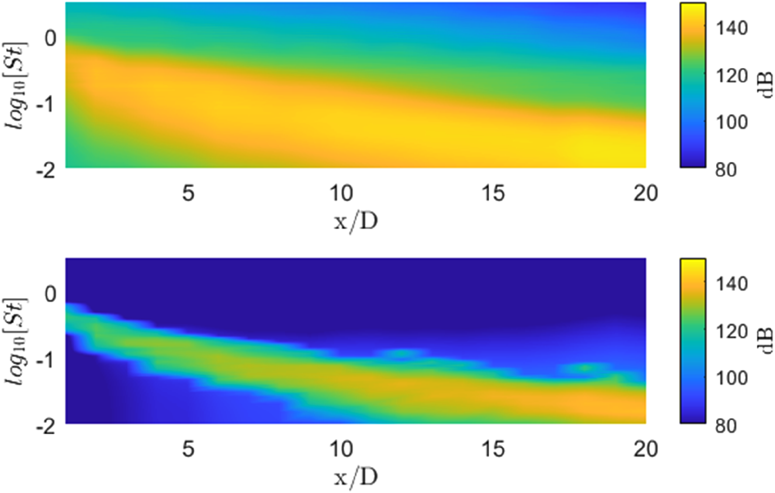
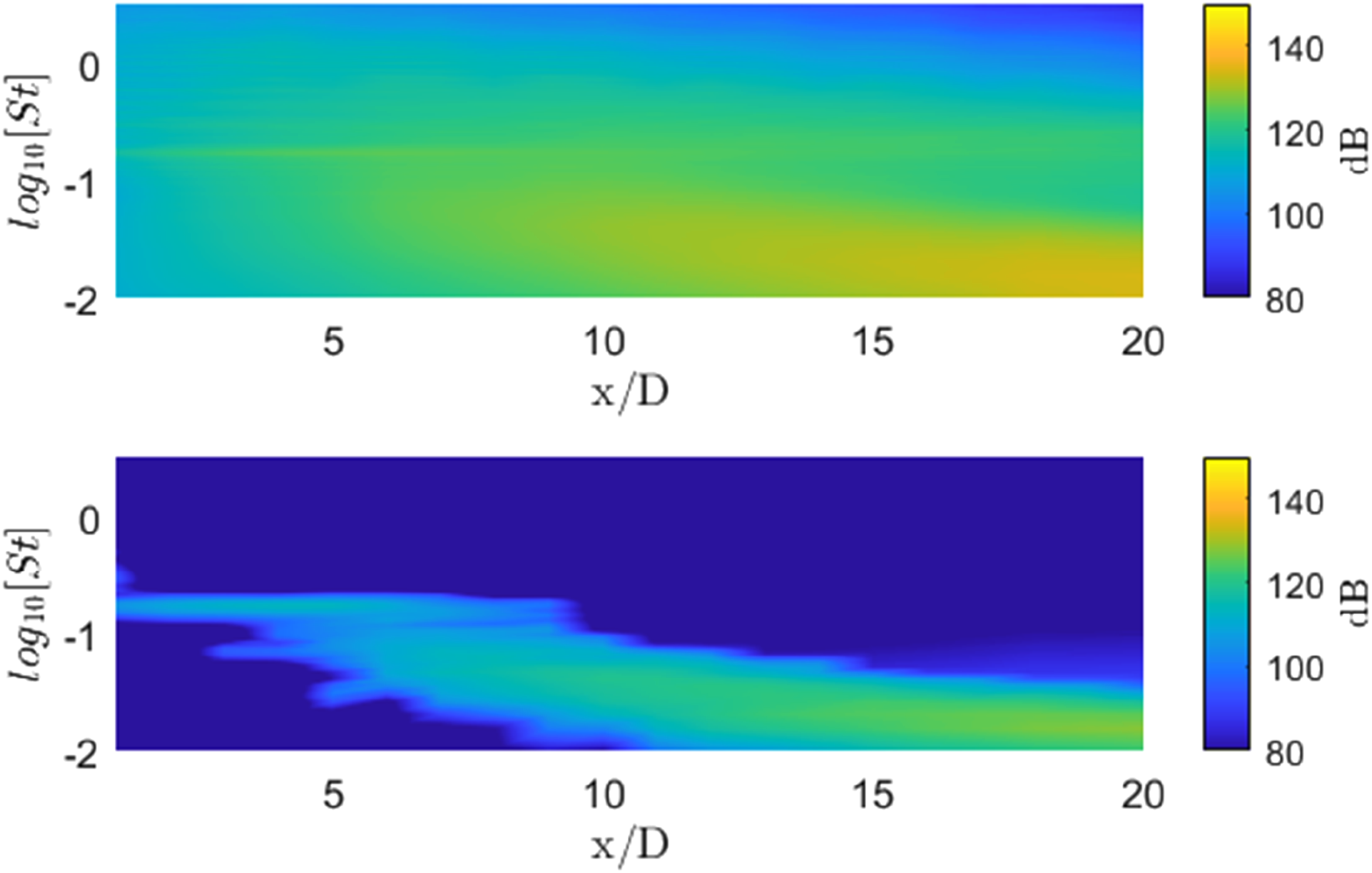
The ability of the MP method to preserve this characteristic has been evaluated, and examples of the results are provided in Figures 7–9, where contour plots of the power spectra are presented in relation to the axial and radial distances. Specifically, the three figures report the SPLs as functions of x/D for cases showing both the effect of M and of r/D. Figures 7 and 8 correspond to a fixed radial distance, r/D=1, and different Mach numbers, M=0.7 and 0.9 respectively. On the other hand, Figure 9 shows results at M=0.9 but at a larger radial distance, r/D=3. In each figure, a comparison between the original spectra (upper plot) and the spectra of the reconstructed signals (lower plot) is reported. It is shown that the energy content evolution is correctly reproduced along with the intensity variations even though, due to the limited number of atoms used in the MP procedure, the reconstructed spectra are more narrow-banded with respect to the original ones. At a fixed radial distance, it is shown that the hydrodynamic pressure is weakly influenced by the Mach number whereas a significant decrease of the energy intensity is observed for the largest radial distance (Figure 9). We note that in this last case, where the hydrodynamic pressure is less intense, a tonal component at St about 0.2, is observed close to the jet exit. We conjecture that this peak can be likely related to the transitional state of the inner boundary layer at the nozzle exit and, consequently, to the frequency of the roll-up of the K-H instability. As shown in the lower plot of Figure 9, both the energy lowering and the trace of the tonal contribution are correctly retrieved by the reconstructed signals mainly in the region close to the jet exit.

Figure 7.

Contour plot of the auto-spectra as functions of the distance from the jet exit (x/D). The upper plot refers to the original signal, the lower plot to the reconstructed ones. Flow conditions are: M=0.7 and r/D=1.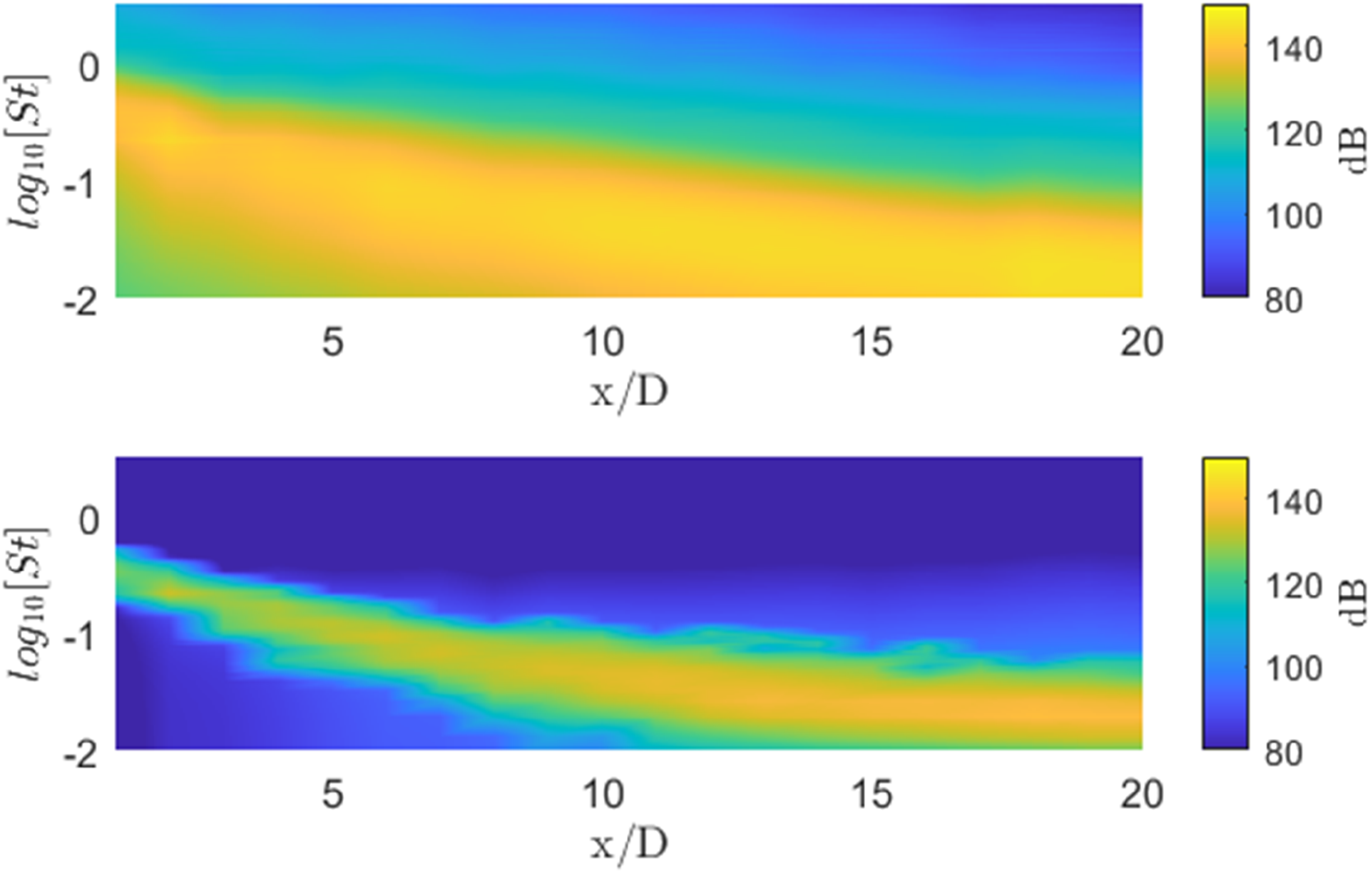

Figure 8.

Figure 9.

The capability of the MP method to preserve the physical properties of the original signals is further explored by analyzing the cross-correlation between near- and far-field pressure fluctuations. This aspect is essential with respect to the purpose of the present study because it is related to jet noise generation and propagation mechanisms.

Examples of cross-correlations are reported in Figure 10 and, consistently with what is done above, the effects of both M and r/D are explored. Some relevant features can be observed. Firstly, we note that, due to the narrow-band nature of the reconstructed signals, the corresponding cross-correlations (the blue lines) exhibit oscillations that are not present in the original cases. Furthermore, since the reconstructed signals have 10% energy content with respect to the original ones, the amplitudes of the correlations computed from the reconstructed signals are much smaller than those of the original ones. Therefore, in order to compensate for this energy difference and facilitate the comparisons, the amplitudes are normalized with respect to their maximum so that each maximum corresponds to a normalized amplitude equal to one.

Figure 10.

Examples of near-far field cross-correlations considering signals reconstructed using 1000 atoms (blue line) compared to the original signals (red line) all taken at x/D=10. (a) M=0.7 and r/D=1; (b) M=0.9 and r/D=1; (c) M=0.9 and r/D=3.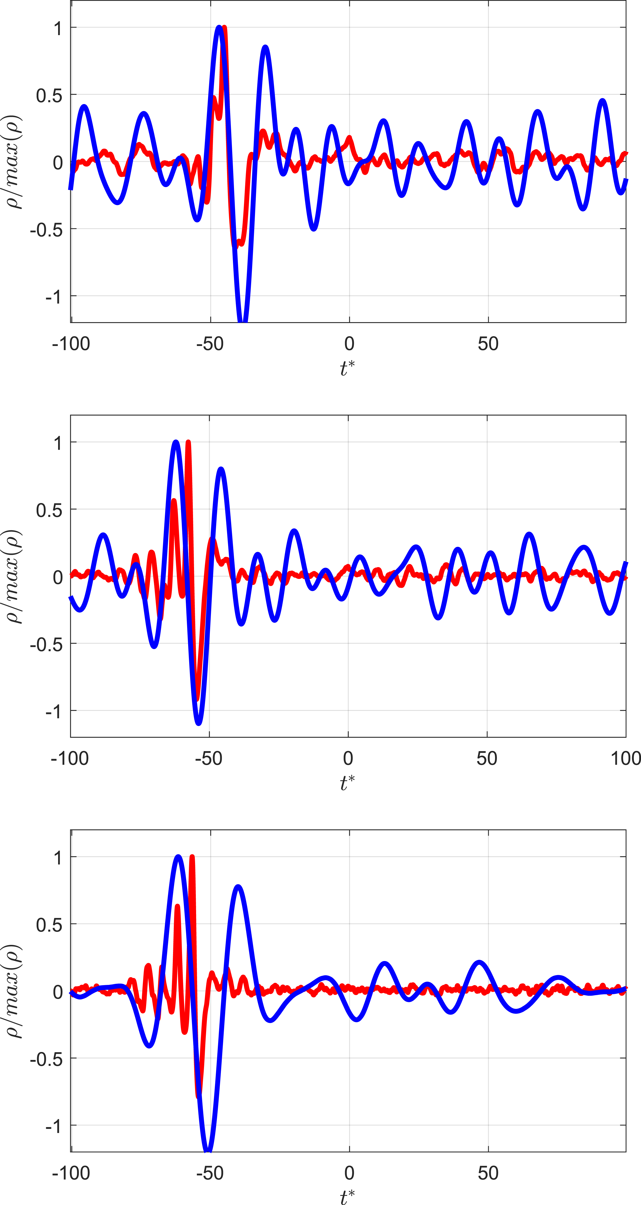

Despite these differences, we note that all the correlations involving the reconstructed signals exhibit a bump, confirming that the relationship between near- and far-field pressures is maintained. Furthermore, the time-location of the maxima is about the same for the original and reconstructed correlations again confirming that the sound propagation mechanism is correctly retrieved. This time-location is related to the acoustic wave propagation velocity and the distance between the selected near-field microphone and the far-field microphone (indicated with $s$ in Figure 1). The cases (a) and (b) correspond to different Mach numbers, and the different time location of the maximum is related to the definition of $t^{*}$ that, as indicated in Figure 5, is based on the mean velocity. Case (c) corresponds to r/D=3 and it is noted that, by comparing with case (b), due to the relevant distance between the near- and far-field microphones, this radial variation has no significant effects on the time location of the correlation maximum. With reference to Figure 1, this corresponds to consider $s \approx h$ .

When the non-dimensional time $t^{*}$ is converted to space, the resulting distance should be consistent with the effective spatial separation between the correlated microphones. This is shown in Figure 11 where the correlations obtained from the reconstructed signals reported in Figure 10, are presented after converting $t^{*}$ to space. This conversion is accomplished by considering a propagation velocity equal to the speed of sound. Therefore, the space s is recovered by the following simple relationship:

t = \frac{t^{*} D}{U} \to s = t \cdot c = \frac{t^{*} D}{U} \cdot c = \frac{t^{*} D}{M}

Figure 11.

Coss-correlations as functions of space considering reconstructed signals at x/D=10. Black line is M=0.7 r/D=1; red line is M=0.9 and r/D=1; green line is M=0.9 and r/D=3. The vertical dotted line highlights the position of the maxima of the three curves.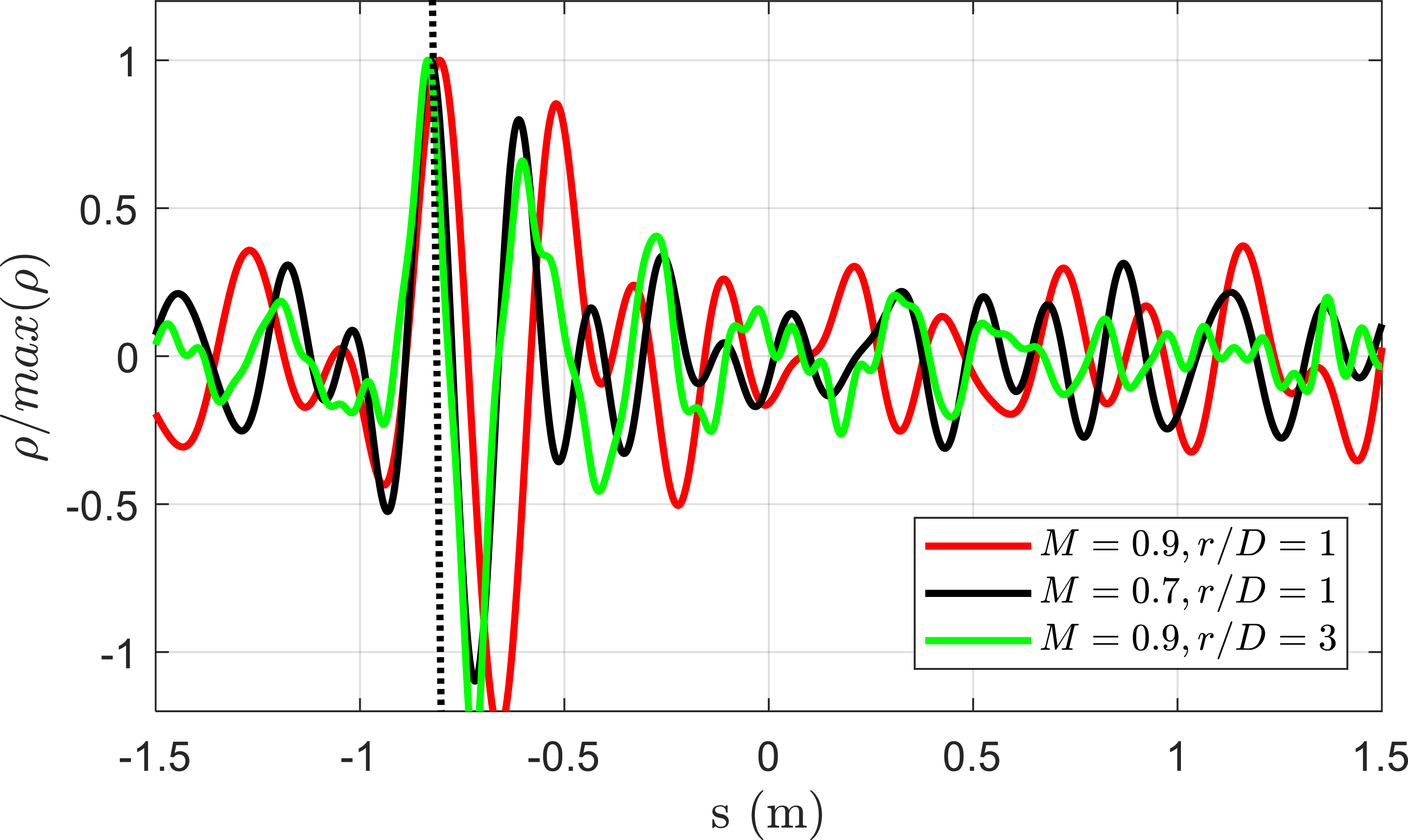

The result of Figure 11 shows that all three maxima occur at the same spatial location corresponding to the effective spatial distance between the near- and the far-field microphones, that is, for the selected near-field microphone, of about 75 cm.

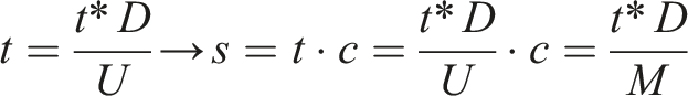
To the purpose of the present study, we further point out the similarity between the original and the reconstructed cross-correlations and the preservation of the near- far-field relationship in the reconstructed signals. This feature is confirmed by extending the cross-correlation analysis to all the axial positions. Contour plots reporting the cross-correlations with the far-field pressure for all x/D and considering the original (upper plot) and the reconstructed (lower plot) near-field pressures, are reported in Figures 12–14.

Figure 12.

Contour plot of near- far-field cross-correlations computed for M=0.7 and r/D=1. The upper plot is referred to the original near-field pressure signals, the lower plot to the reconstructed ones.

Figure 13.

Contour plot of near- far-field cross-correlations computed for M=0.9 and r/D=1. The upper plot is referred to the original near-field pressure signals, the lower plot to the reconstructed ones.

Figure 14.

Contour plot of near- far-field cross-correlations computed for M=0.9 and r/D=3. The upper plot is referred to the original near-field pressure signals, the lower plot to the reconstructed ones.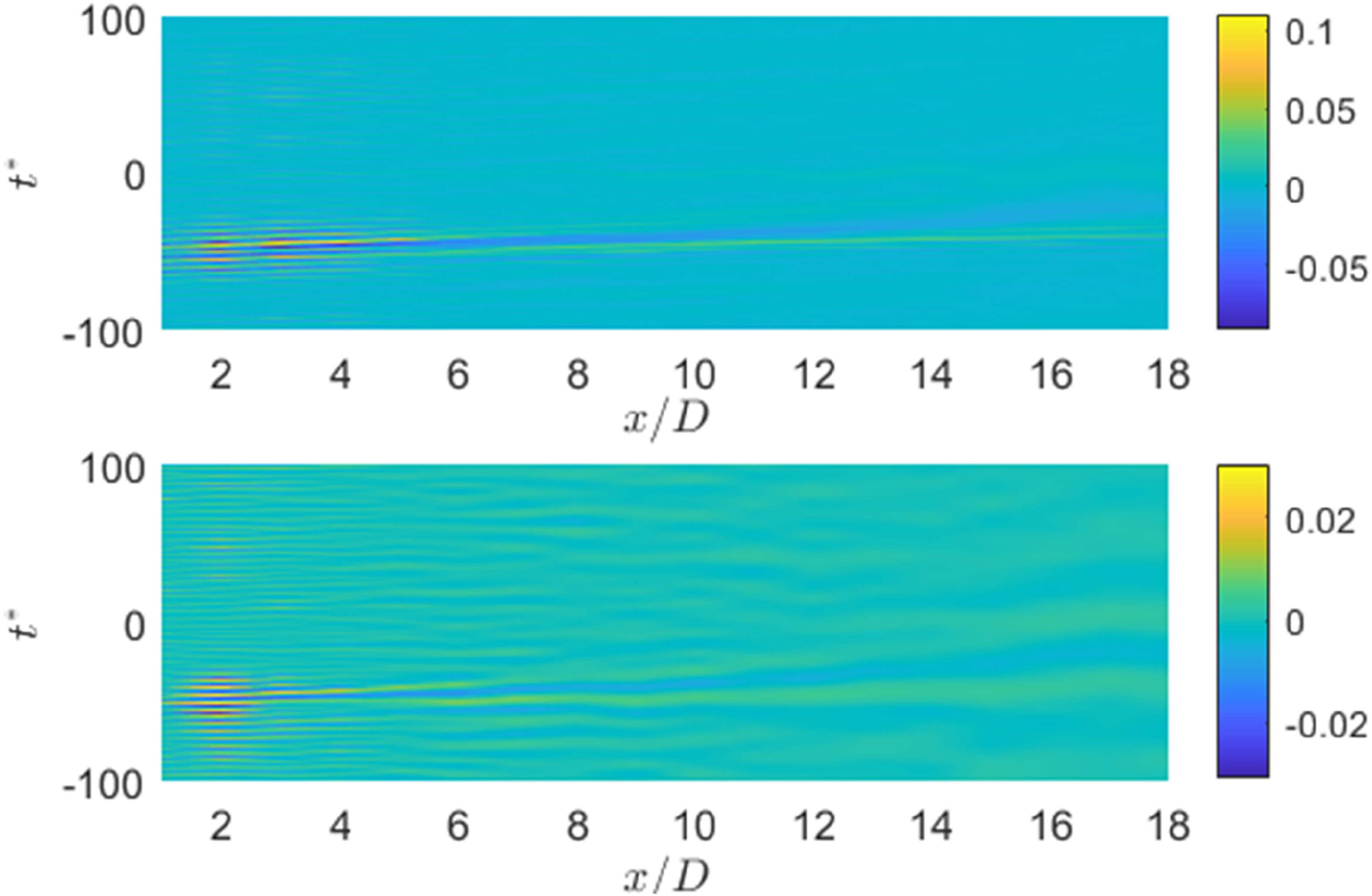

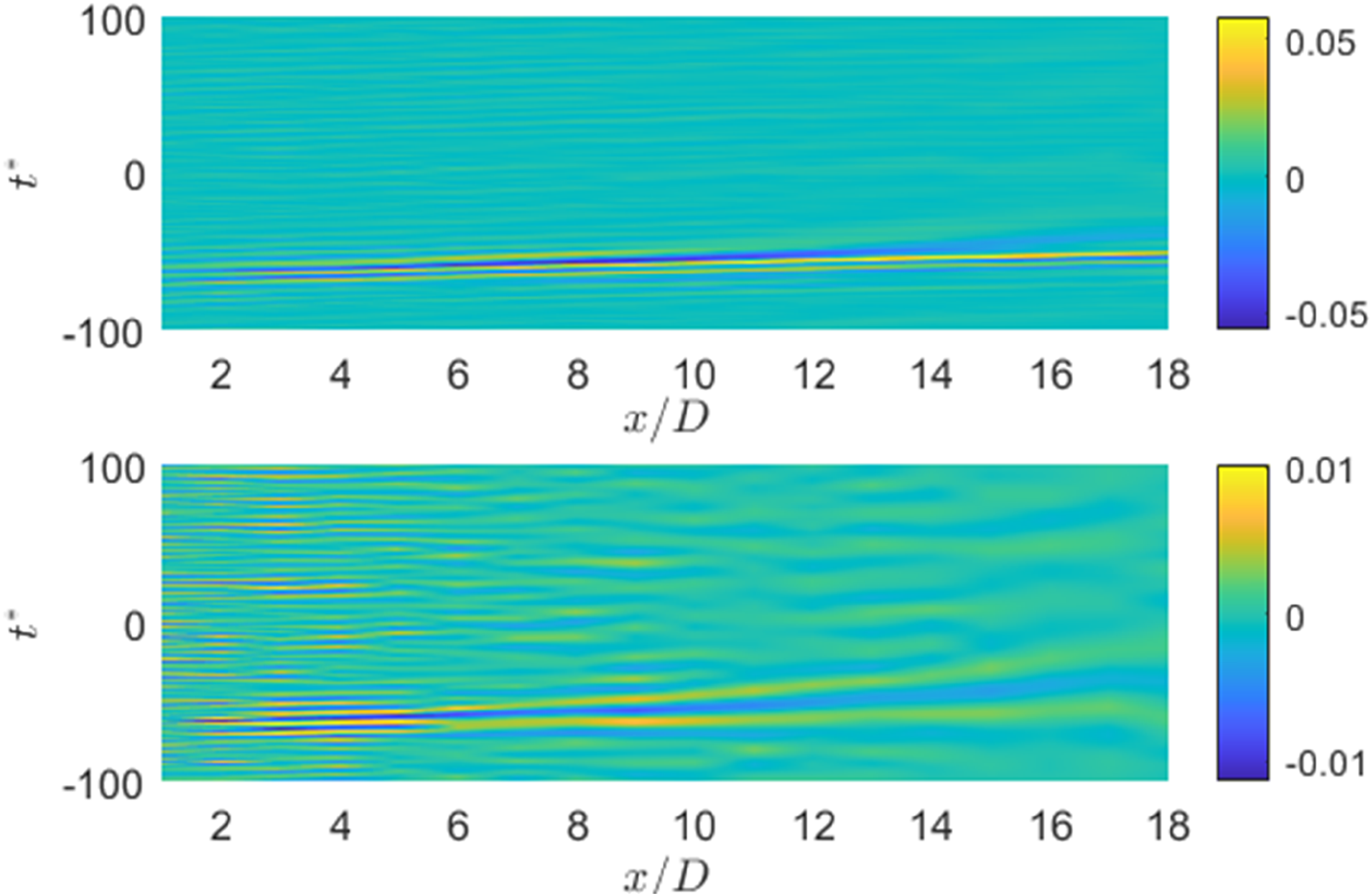
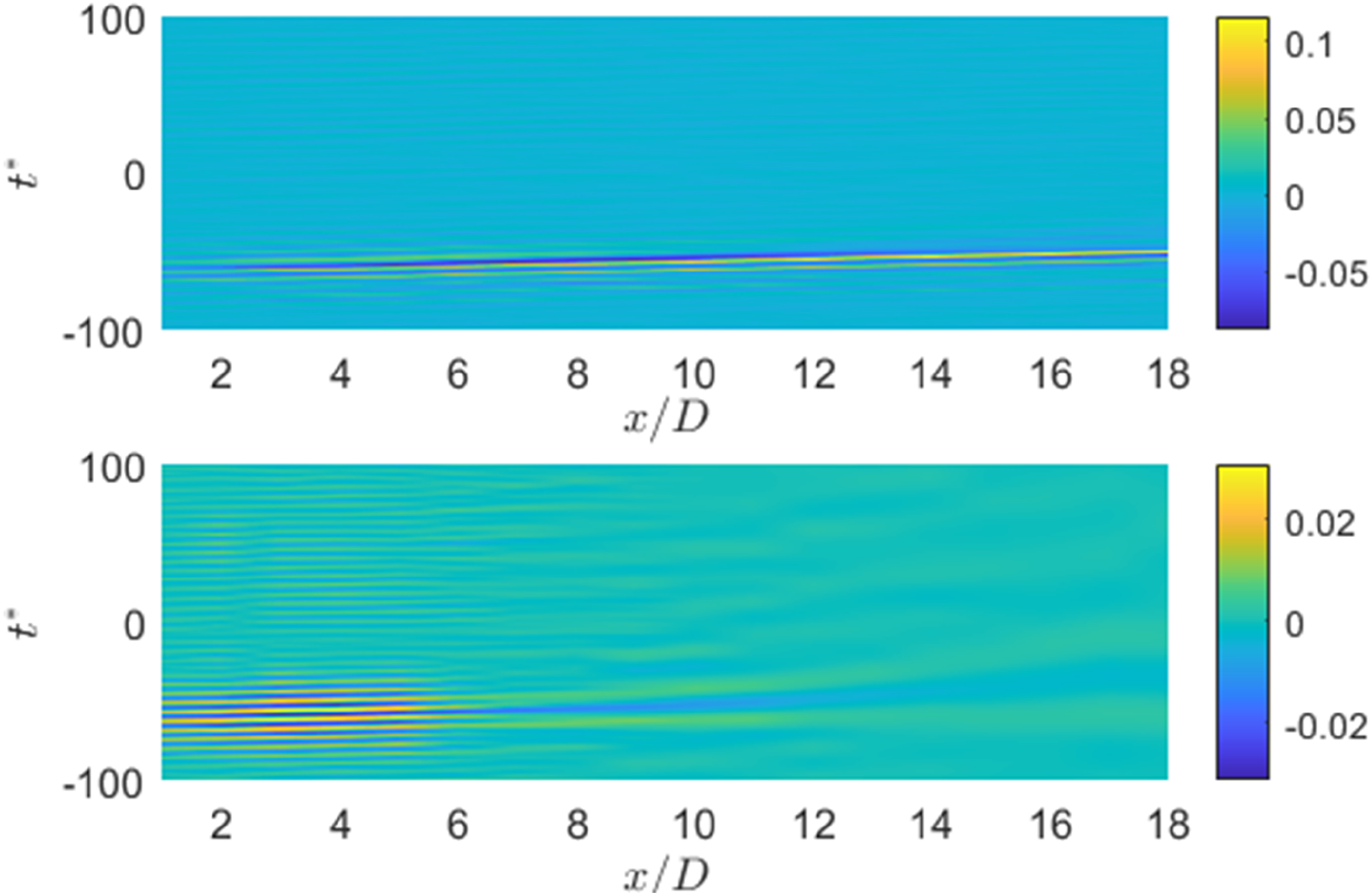
As outlined above, the general features are preserved in particular for what concerns the location of the correlation maxima, that is related to the propagation of acoustic waves from the near- to the far-field microphone. All the plots allow for the identification of the correlation bump and of its time location. This parameter changes with x/D as an effect of the different position of the near-field microphone along x/D and thus of the different distances $s$ with respect to the fixed far-field microphone. With reference to Figures 13 and 14, relevant differences between the original and reconstructed correlations are observed at large $x / D$ . This is related to the use of a few Gabor functions that allows for a reasonable reconstruction of the signal in the region close to the jet exit, where the flow is quasi-deterministic, but it is insufficient to accurately reproduce the highly turbulent far region. Nevertheless, the evolution of the cross-correlation bump, which is the main feature targeted by the reconstruction, is qualitatively well captured also at large axial distances.

On the other hand, in the region close to the jet exit, we note, especially at the highest M (Figures 13 and 14), a significant amplitude of the oscillations. This behavior is evident in the reconstructed correlations around $x / D < 5$ , corresponding to the jet potential core extension. The observed behavior suggests that in this region, the measured signals compress well onto the basis of Gabor functions leading to an enhancement of the effect of the oscillatory mechanism clearly visible in the near-field pressure signals. When $x / D$ increases, the shear layer becomes less coherent and after the end of the potential core, the jet becomes fully turbulent and, hence, with a more stochastic behavior.

This interpretation is further supported by Figure 15 where correlations are reported in such a way to enhance the presence of the oscillatory behavior and its progression as a function of the distance from the jet exit. It is clear that the oscillations are much more pronounced when the correlations are computed using the near-field reconstructed signals compared to those computed using the original ones. In case (a), where the original signals are considered, some oscillations are present, but the shape of the correlations seems to be weakly dependent upon $x / D$ . On the other hand, the reconstructed signals of the case (b) exhibit high amplitude oscillations from the jet exit only up to $x / D = 5$ , and after that distance the shape of the correlations changes significantly.

Figure 15.

Cross-correlations between the near-field and the far-field signal at M=0.9 and r/D=3. (a) Original near-field pressures; (b) Reconstructed near-field pressures.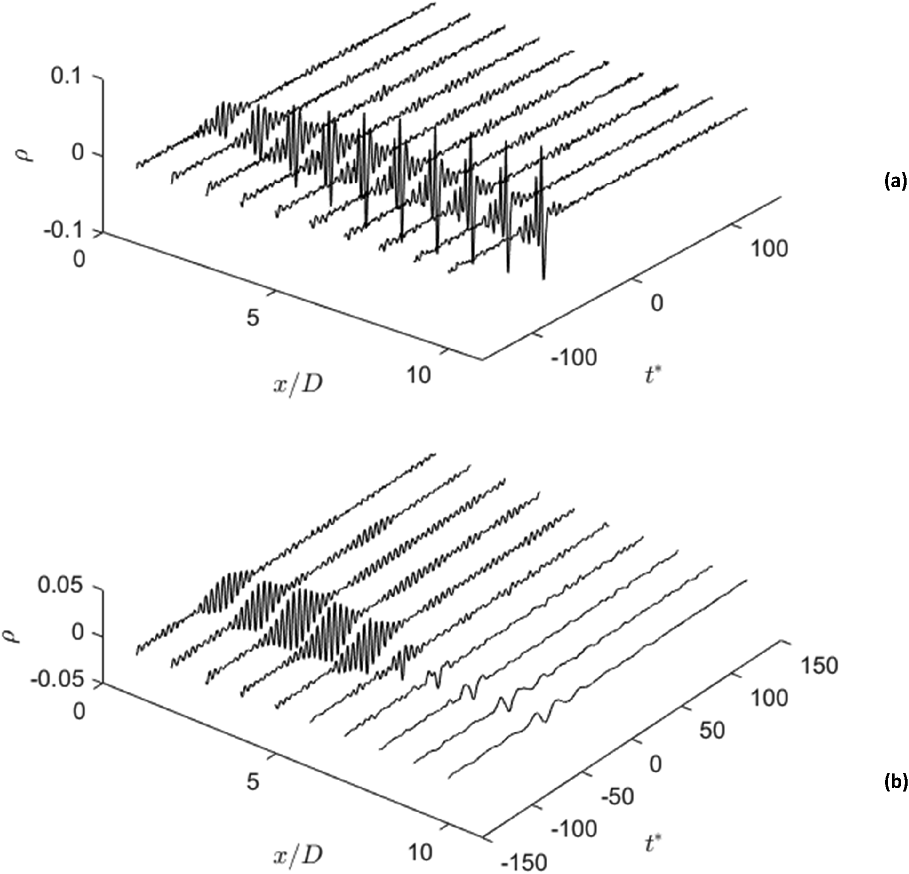

The case reported refers to M=0.9 and $r / D = 3$ but similar results are obtained in all the other configurations and are not reported here for brevity. This result further demonstrates the capability of the MP method to provide a simplified reconstruction of signals preserving their relevant properties related to the flow physics.

Conclusions

In this paper, the MP decomposition is applied to experimental pressure signals measured in the near- and far-field of a high Reynolds number compressible jet. The primary objective of this work is to demonstrate that the MP approach can provide a simplified representation of complex jet noise data and can be used effectively for reduced-order modeling. The procedure for the reconstruction of the pressure signals is accomplished through the superpositions of a rather limited number of Gabor functions composing the Dictionary. Only one thousand atoms are selected, this number providing reconstructed signals with an energy content corresponding to about 10% of the original ones. We show that the modeled signals preserve the relevant features of the original signals, particularly those related to the jet noise generation mechanisms and the propagation of acoustic waves in the far field. These properties have been exploited by the computation of spectral features and of near/far-field pressure cross-correlations as well as by the comparisons with the results obtained using the original data. We note that, in principle, employing an infinitely large number of atoms in the MP algorithm would lead to a perfect reconstruction of the original signal. By using a very limited number of atoms, the differences observed in the spectral and temporal features, when comparing the reconstructed signals to the original ones, may appear significant. However, these differences can be minimized simply by increasing the number of atoms. The present investigation has demonstrated that, even with a small number of atoms, it is possible to capture key features of the original signals. These include accurately identifying the high-energy region in the spectral domain (although not its amplitude), as well as monitoring its evolution in $x / D$ and its dependence on M. Additionally, the method successfully detects the correlation bump in the time domain, again without accurately reproducing its amplitude, and captures its evolution across $x / D$ and M.

The possibility of representing a very complex, non-deterministic signal through the superposition of much simpler waveforms, opens new perspectives in the field of reduced-order modelling to describe the jet-flow dynamics. One of the key aspects to be clarified in future work is the relationship between the proposed simplified description of the near-field pressure and the acoustic propagation and scattering processes that are characteristic of jet noise. To achieve this, a more detailed characterization of the far-field pressure is necessary, and we are currently conducting new measurements combined with the analysis of additional, more comprehensive jet noise datasets. The availability of a more detailed description of the far-field pressure would also allow to test the MP decomposition on the far-field pressure distribution and to investigate further the capability of the method to recover correctly important physical features correlated to the acoustic field. Furthermore, examining spatial features through PIV measurements or numerical simulations would offer valuable insights into the physical mechanisms underlying the observed temporal behavior. The achievement of these ambitious objectives will be the focus of future research efforts.

Footnotes

ORCID iDs

Roberto Camussi

Elisa De Paola

Funding

The authors received no financial support for the research, authorship, and/or publication of this article.

Declaration of conflicting interests

The authors declared no potential conflicts of interest with respect to the research, authorship, and/or publication of this article.

References

Lighthill

Newman

MHA

. On sound generated aerodynamically I. General theory. Proceedings of the Royal Society of London. Series A. Mathematical and Physical Sciences 1952; 211(1107): 564–587.

Mertins

. Signal analysis: Wavelets, filter banks, time-frequency transforms and applications. John Wiley & Sons Ltd, 1999.

Grosveld

Sullivan

Rizzi

. Temporal characterization of aircraft noise sources. 42nd AIAA Aerospace Sciences Meeting and Exhibit. Reno, Nevada, 5-8 January 2004.

Mayer

Zang

Azarpeyvand

. Aeroacoustic investigation of an oscillating airfoil in the pre- and post-stall regime. Aero Sci Technol 2020; 103: 105880.

Antoni

Leclère

Dinsenmeyer

, et al. Standalone extraction of tonal components from aeroacoustic signals. AIAA J 2022; 60: 844–859.

Guj

Camussi

. Statistical analysis of local turbulent energy fluctuations. J Fluid Mech 1999; 382: 1–26.

Mancinelli

Pagliaroli

Di Marco

, et al. Wavelet decomposition of hydrodynamic and acoustic pressures in the near field of the jet. J Fluid Mech 2017; 813: 716–749.

Jawahar

Meloni

Camussi

, et al. Intermittent and stochastic characteristics of slat tones. Phys Fluids 2021; 33: 33827.

Mallat

Zhang

. Matching pursuits with time-frequency dictionaries. IEEE Trans Signal Process 1993; 41: 3397–3415.

10.

Ray

Crone

Niebur

, et al. Neural correlates of high-gamma oscillations (60–200 Hz) in macaque local field potentials and their potential implications in electrocorticography. J Neurosci 2008; 28: 11526–11536.

11.

Durka

. Matching pursuit and unification in EEG analysis. Artech House, 2007.

12.

Jabbari

Ghassemian

. Modeling of heart systolic murmurs based on multivariate matching pursuit for diagnosis of valvular disorders. Comput Biol Med 2011; 41: 802–811.

13.

Zhang

. Matching pursuit parallel decomposition of seismic data. Comput Geosci 2017; 104: 54–61.

14.

Bergh

. Deconvolution approach to the mapping of acoustic sources with matching pursuit and matrix factorization. J Sound Vib 2019; 459: 114842.

15.

Padois

Berry

. Orthogonal matching pursuit applied to the deconvolution approach for the mapping of acoustic sources inverse problem. J Acoust Soc Am 2015; 138(6): 3678–3685.

16.

Bousabaa

Bulté

Mincu

D-C

, et al. Sparse green’s functions estimation using orthogonal matching pursuit: application to aeroacoustic beamforming. AIAA J 2018; 56(6): 2252–2270.

17.

Bruneau

Fischer

Peter

, et al. Comparison of numerical methods for the computation of energy spectra in 2D turbulence. Part II: adaptative algorithms. Sampl Theory Signal Image Process 2005; 4: 271–280.

18.

Davis

Mallat

Zhang

. Adaptive time-frequency approximations with matching pursuits. In: Chui

Montefusco

Puccio

(eds). Wavelets: Theory, Algorithms, and Applications. Academic Press, 1994, vol 5, pp. 271–293.

19.

Chen

Donoho

Saunders

. Atomic decomposition by basis pursuit. SIAM Rev 2001; 43(1): 129–159.

20.

Durka

Ircha

Blinowska

. Stochastic time-frequency dictionaries for matching pursuit. IEEE Trans Signal Process 2001; 49(3): 507–510.

21.

Kuś

Różański

Durka

. Multivariate matching pursuit in optimal Gabor dictionaries: theory and software with interface for EEG/MEG via Svarog. Biomed Eng Online 2013; 12(1): 94.

22.

Mineault

(2024). Matching pursuit for 1D signals.

23.

Grizzi

Camussi

. Wavelet analysis of near-field pressure fluctuations generated by a subsonic jet. J Fluid Mech 2012; 698: 93–124.

24.

Camussi

Mancinelli

Di Marco

. Intermittency and stochastic modeling of hydrodynamic pressure fluctuations in the near field of compressible jets. Int J Heat Fluid Flow 2017; 68: 180–188.

25.

Suzuki

Colonius

. Instability waves in a subsonic round jet detected using a near-field phased microphone array. J Fluid Mech 2006; 565: 197–226. https://api.semanticscholar.org/CorpusID:13087343