Multi-algorithm approach for identification of structural behavior of complex structures under cyclic environmental loading

Abstract

In the past years, an increasing number of structures have been equipped with permanent monitoring systems, able to record the structural response in terms of displacements and strains over very long periods of time, and theoretically, for the entire life of the structure (Structural Health Monitoring). Despite the high number of applications, to date, very few studies have been presented aimed at interpreting the data, in particular, when the spatial and behavioral complexity of the structure under investigation requires a non-model-based approach. This article shows that the interpretation of data from a long-term static monitoring can be very helpful for the comprehension of the structural behavior under complex interaction structure–environment. The discussion aims at underlining that a scheduled and unique procedure is very hard to define depending on the great variety of structures and applications and on the right identification of the parameters able to explain structural degradation evolutions or sudden changes. In these cases, a multi-step algorithm with different signal processing techniques applied in cascade seems to be the only reliable approach. The proposed procedure will be carried out using available data from the long-term monitoring of a quay wall in the Port of Genoa, in Italy, but it can be generalized to several structures under cyclic environmental loading (tides, temperature, etc.). The characterization of the structural behavior under temperature variations will be used here to define the representative features of the quay. Once defined, these parameters will provide a means for detecting and localizing the insurgence of damage or material degradation from the measurements.

Keywords

signal processing analysis quay structures cyclic loading statistical analysis damage-sensitive features

Introduction

The economical effort of building, replacing, or retrofitting infrastructures is becoming more and more important in industrialized countries, where the existing infrastructure stock is subjected to aging and obsolescence. For example, the majority of the transportation infrastructures existing in Europe and in the United States have been built from the 1950s to the 1970s, when features of the traffic intensity and loads were significantly different from the current features and when some of the phenomena related to material degradation were not fully discovered or understood.¹^–³ Moreover, the problem is not confined to transportation infrastructures, but also includes other types of infrastructures like energy production and distribution systems, water supplies and wastewater treatment plants, communication facilities, schools, hospitals, homeland defense, harbor installations, etc.

For special classes of structures or for specific environmental situations, models used in design practices may not cover the wide range of problems that need to be solved when assessing the safety conditions of the structure as built. This is, particularly, true for large structures in aggressive environments, like bridges in coastal or mountain areas and marine structures,⁴ or in the case of prevention of pollution loads discharged from distribution networks.⁵ In all these cases, observation of the structural behavior and/or of the environmental parameters with an adequate monitoring system can cover the gap between the reality and the theoretical models that have been developed for the design to obtain a picture of the structural state and evolution.

The continuous development in sensor technology and data acquisition systems makes possible the realization of complex permanent instrumental monitoring systems; they are able to monitor the most significant parameters of structural response under external loads and environmental conditions, enabling, in principle, a continuous evaluation of the actual safety conditions of such structures and finally a data-based reliability analysis.⁶ Through these large-scale monitoring projects, a considerable amount of data can be available, so that data analysis and interpretation play a very important role in structural health monitoring (SHM) research.

Thanks to these recent technologies, the field of continuous monitoring is facing the research community since the last years, while the periodic monitoring of dynamic parameters has been largely investigated in the past.⁷ Usually, the measured structural features are used to construct a mechanical model that is later updated using monitoring data. The mechanical model can be used for: (a) reliability analysis and/or (b) damage identification. Recently, the integration of the reliability analysis with the long-term SHM has been attempted⁸^–¹¹ and improved by including the uncertainty propagation in the assessment process.^12,13 On the other hand, the mechanical model is very useful also to extract the structural features (static or dynamic) that are sensitive to damage or material degradation. For example, regarding the inverse problem of detecting a single open crack in an elastic straight beam in bending, dynamic identification techniques provide explicit expressions for the position and the severity of the crack; by the way, the methodology is valid only for small damages and for initially uniform beams under special boundary conditions (pinned–pinned, sliding–sliding).¹⁴ Other models reconsider the inverse problem of detecting a single crack in an elastic straight beam in bending from static measurements to provide explicit expressions for its position and its severity, which represent the exact solutions of the inverse problem.¹⁵ However, these are above all theoretical approaches, because the meaning of data from a real monitoring is usually not clearly associated to any mechanical model of structural response, due to the particularity of the instrumented structures and their boundary conditions and loads.

Recent literature¹⁶ has put into evidence that theoretical and lab knowledge needs to be transferred to real structures to control static or dynamic parameters during in-service conditions. In particular, for large structural systems interacting with their environment, safety and operability of the system depend on phenomena involving not only structural behavior, but also coupled structure–environment responses. Moreover, due to the inherent geometrical and physical complexities of the problem, model-based diagnosis can be seldom invoked, and translation of measurement data into valuable information shall be based mostly on engineering judgment and on mathematical processing of the instrumentation signals. In addition, when monitoring systems are installed not at the beginning of the life-cycle of the structure but at a later stage (repair for instance), major modifications of the structural system may have occurred because of the effect of loads and other external causes, or because of human intervention. This aspect has a great influence on data analysis and interpretation, because of the greater role that uncertainties do play in this case.¹⁷

The automatic detection of damages from continuous static monitoring is still a challenge. The measured quantities during continuous monitoring are typically displacements or strains under operational and environmental loads. Practitioners have difficulties in choosing the best data processing approach for each application. Scientifically, the most successful methods are not yet identified, even though a great number of signal processing algorithms have been investigated. Moyo and Brownjohn¹⁸ proposed the detection of anomalous structural behavior using discrete wavelet analysis. Experimental studies on structural damage identification based on wavelet packet transform have been done with good results.¹⁹^–²¹ In SHM, one of the most common model-free methods for damage detection is based on autoregressive analysis. In their general version, these methodologies consist of expression of a time series as a linear function of its past values and the past values of exogenous variables. The estimation of the parameters is done continuously and damages are normally discovered if a significant variation in the parameters appears.²²^–²⁷ The linear regression method has also attracted a notable interest because of its simplicity and wide applicability. However, this methodology may be prone to a harmful affect in case where data are used with outliers, a common problem observed during real monitoring. Outliers’ accommodation methods are well known by robust methods, where robustness is given by statistical procedures insensitive to outliers. In this framework, robust regression analysis has been proposed and applied in the field of structural monitoring.²⁸^–³⁰ The Correlation Anomaly Scores Analysis has been proposed for change analysis of correlated multi-sensor systems using a neighborhood preservation principle.³¹ The goal of change analysis is to compute the anomaly score of each sensor when it is known that the system has some potential difference from a reference state. If the system is working normally, the neighborhood graph of each sensor (defined using the correlation between sensor measurements) is almost invariant against the fluctuations of experimental conditions. Deraemaeker et al.³² presented a complex methodology for damage detection under changing environmental conditions. The effects of environment are treated using factor analysis and damage is detected using statistical process control with the multi-variate Shewhart-T control charts. Posenato et al.³³ proposed a methodology based on moving principal component analysis (MPCA); a comparative study with other signal processing algorithms has shown that for quasi-static monitoring of civil structures, the proposed methodology performs better than wavelet methods, Short Term Fourier Transform and Instance-Based Method, also in case of noise, outliers, data missing, and database with different sensor typologies.^34,35

In the section ‘The San Giorgio pier,’ the discussion on the complexity of data processing will be carried on by means of available data from the real long-term monitoring of a quay wall in the Port of Genoa, Italy.³⁶ Section ‘Strategy for data analysis’ tries to give a generally valuable strategy for data processing through a multi-algorithm approach. Sections ‘Classification of block behavior,’ ‘Damage-sensitive feature for blocks of type 1,’ and ‘Damage-sensitive feature for blocks of type 2’ emphasize the preliminary steps aimed at understanding the mechanical response of such a complex structure under cyclic loads in terms of representative features of the quay. As a matter of fact, in the field of structures with a strong random behavior, it is necessary to develop a mechanical-probabilistic model through available data from SHM. This can be relatively easy if the structure is subjected to cyclic actions because its random behavior can be identified using the information from loading cycles. In particular, in this article, focus will be placed on the monitoring of evolutionary phenomena, taking place in structures as a result of the interaction with environment and operational loads.³⁷ Due to the large amount of instrumented blocks, in this application, the statistical analysis has proved to be successful for the identification of the typical response features. The second part of the proposed multi-algorithm analysis will be aimed at giving information on the structural health conditions. Using the previously identified response parameters as deterioration-sensitive features, section ‘Damage detection’ presents the linear regression algorithm as an effective damage detection algorithm and applies it to the available data to successfully detect and localize the insurgence of damage or material degradation in the monitored quay.

The San Giorgio pier

The monitoring program

The San Giorgio pier is used for coal import and it has been subjected to a retrofitting program to increase the water depth of the nearby basin. The facility has been built in the 1920s and the vertical walls delimiting the quays are made of heavy concrete blocks. Dredging has required strengthening of the wall: the structure has been underpinned with jet-grouting columns, and the blocks have been connected by means of vertical steel rods. Stability has been improved with permanent active tendons installed along the entire length of the pier.³⁸

The crown block of the San Giorgio pier was equipped in 1999 with an array of 67 SOFO fiber-optic strain sensors,³⁹ located in a service tunnel along the top blocks, in such a way to have 3 longitudinal sensors in 24 measuring sections, named measuring blocks in the following. The generic block cross-section (left) and the schematic longitudinal view (right) of the equipped pier are represented in Figure 1. Each sensor has an active length of 10 m. The monitoring had the goal to detect possible distress caused by dredging activities in the adjacent basin and also to run a long-term health monitoring experience, as a first step of a larger project aimed at establishing a decision support system for maintenance operations of the Port facilities.³⁶

Figure 1.

Sensor installation along the quay for 19 measuring blocks (right) and block cross-section (left) with sensor position inside the service tunnel (measurements in cm). The thick vertical lines represent two possible locations of the dilatation joints along the pier (section ‘Understanding of mechanical behavior’).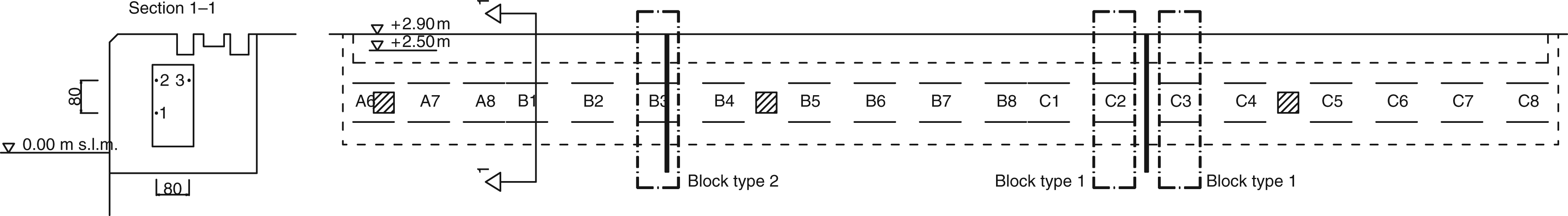

Acquisition campaigns were programmed four times a day to analyze the main variations of temperature during 24 h (by day and by night) and with greater reason, weekly and seasonal variations. The system was fully operational for 4 years (from November 1999 to October 2004), with the exception of some interruptions due to the maintenance on the system and other management reasons (Figure 2). This monitoring time is a common lifetime for operational systems near the sea.³⁷

Figure 2.

Example of time histories for some measuring blocks during the whole monitoring period.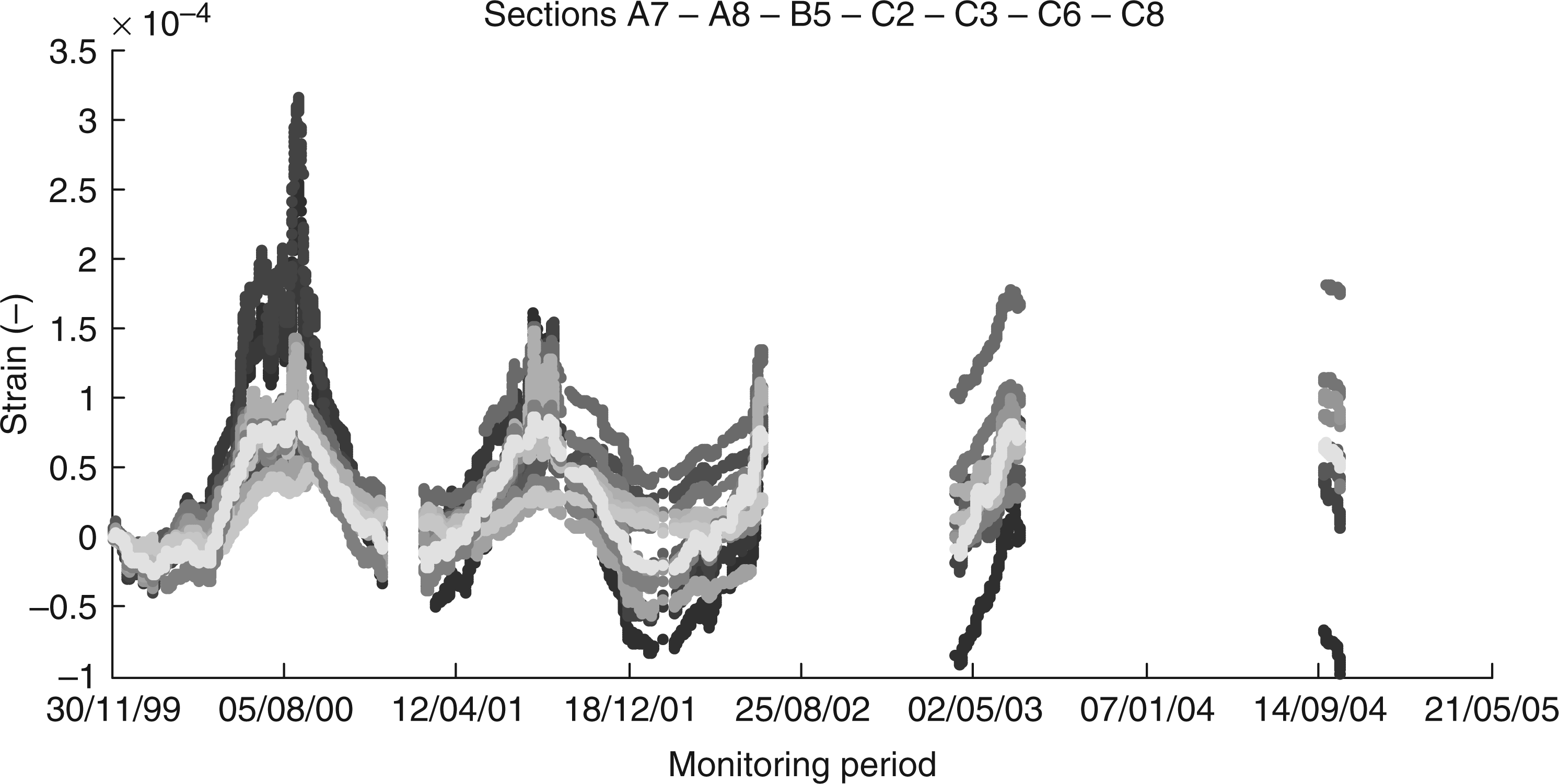

Understanding of mechanical behavior

In order to choose the best approach for data interpretation, it is useful to understand if the structure has a well-defined mechanical behavior and if damage mechanisms can be clearly described. The different layers of concrete blocks are linked each other, thanks to the gravity force. After the reinforcement works, the blocks should have a higher connection rate due to the distributed vertical steel rods. For these reasons, it can be supposed that the structure behaves as a monolithic structure, so that great displacements interesting the underwater layers are transferred to the superior layers until the crown block. Indeed, the installed monitoring system is able to measure the crown block displacements.

On the other hand, the crown block can itself experience small displacements induced by external temperature variations and sea level changes. The horizontal relative displacements between blocks are allowed, thanks to the presence of dilatation joints along the pier (Figure 1). However, the conditions and the position of joints are unknown because most of them are completely filled by coal dusts and it is not clear if they behave properly as dilatation joints. In addition, the crown block should not be allowed to expand freely with thermal variations due to the continuous support of the lower block.

It can be concluded that the structure under investigation is strongly non-homogeneous due to the interaction between old structural elements and new strengthening elements. The structure is characterized by spatial and behavioral complexity and possible variations in the structural behavior or damages are expected to occur as a result of complex phenomena. The study of a reliable numerical model of the pier is very complex and it would require a lot of hypothesis and simplifications. Thus, data interpretation will have to resort to statistical algorithms for gathering some information on the structural behavior.

Strategy for data analysis

Key factors

Fixed marine structures are primarily designed to withstand environmental and operational forces. The main phenomena in the marine environment able to produce changes in the structural response and loss of functionality can be:

corrosion of steel and degradation of concrete and other materials;

crane movements and operations that can cause overloads on the quays;

interaction with sea actions, for example tide and wave actions;

moored ships, also in case of collision;

interaction with environmental parameters, such as temperature, solar radiation, and wind.

Internal structures in a port environment, such as piers, docks, berths, dolphins, transportation facilities, and buildings, are not usually designed to withstand sea actions, because wave actions are absorbed by the protection facilities. In addition, tides are not a phenomenon of interest in the Mediterranean area and for this reason they have not been considered as a key factor for the San Giorgio pier analysis.

The relationship between the measured strains and the presence of the moored ship has been here investigated. It is also related to the crane operations for the goods uploading and downloading. No clear correlation with the moored ships has been identified (Figures 3 and 4).

Figure 3.

Strain time history of sensor C82 and temperature variations. Black crosses represent measurements performed with the moored ship.

Figure 4.

Zoom of the black rectangle in Figure 3.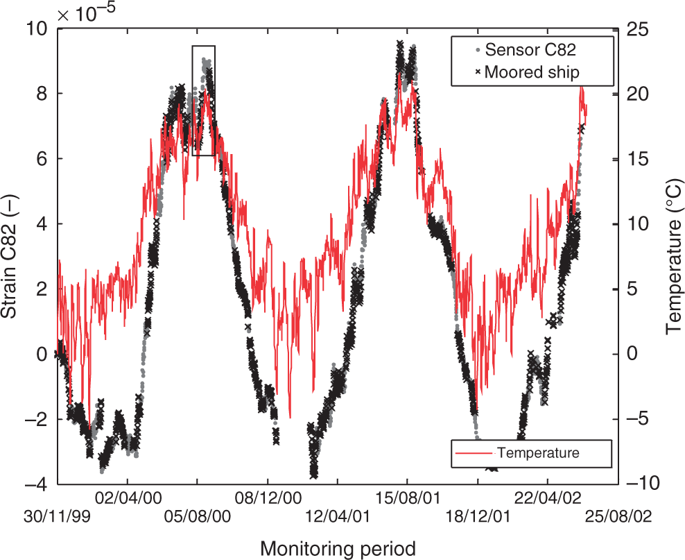

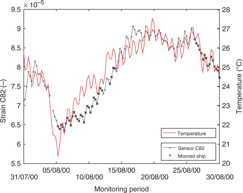
On the contrary, the time histories of Figure 3 and the zoomed Figure 4 show that a strong correlation with thermal variations exists and the following analysis will be mainly focused on temperature actions.

Steps of the analysis

A multi-step algorithm is here proposed for a generally valuable data processing. The proposed algorithm cannot be completely independent of key factors analysis (section ‘Key factors’) and of the expert’s judgment as it is completely data driven and some starting assumptions are necessary. The focus issue regards the choice of: (a) one or more reference measuring blocks and (b) a training period. The reference measuring blocks can be selected by observing the stability and the regularity of the measured variables during the monitoring period. The reference measuring blocks should be, as most as possible, stationary with time. The training period is a time period that can be assumed as a reference period for comparison with further monitoring periods. When the parameter under observation has a cyclic trend, the training period should contain at least one complete cycle. As a consequence, the evaluation of the right training period depends on the governing load or action and on the corresponding periodicity of the measured variables; as in the case of San Giorgio pier, when cyclic loads, for example temperature variations, play the most important role, at least 1 year of observation is required to make the analysis independent of the seasonal variations, as it will be demonstrated in the section ‘Measuring blocks of type 1’.

The flow chart in Figure 5 suggests a sequence of signal analysis algorithms to be applied in cascade for the continuous monitoring of a structure with characteristics similar to the pier under study, and the information that can be drawn out without using any numerical structural model. This flow chart is representative of the processing steps performed for the San Giorgio pier and presented in the following sections. Three main steps are highlighted with bold type and listed on the right side of the flow chart: (1) classification of measuring blocks behavior, (2) identification of damage-sensitive features for the specific application, and (3) damage detection. A dashed rectangle groups the ensemble of the actions and tests to be performed for each step of the processing. The input data and the output results of the multi-algorithm flow chart are pointed out using a parallelogram.

Figure 5.

Flow chart of the data processing steps.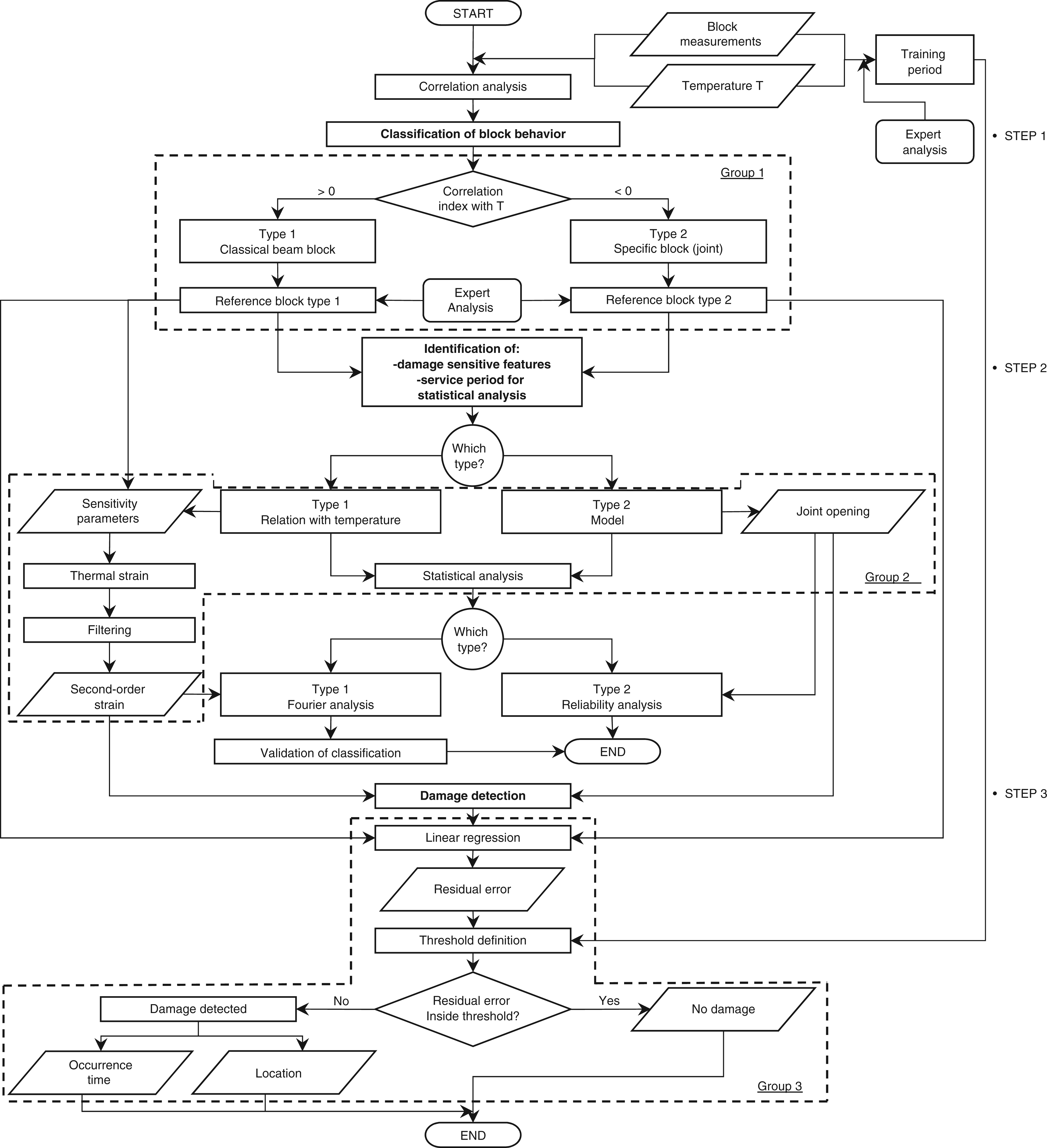

Classification of block behavior (group 1 in Figure 5)

The analysis has been focused on the first 2 years of measurements (Figure 2), because they are almost complete (only 603 data missing on a total of 3776 measurements). The measurement campaigns with some data missing have simply not been considered in the analysis and they are assumed not to alter the results. This assumption is rather consistent because data missing are not concentrated in the same period.

Two mechanical behaviors can be identified from the data:

The behavior in the direction normal to the block cross-section mainly due to dilatation. It can be assumed that this behavior is homogeneous for all measuring blocks because sensors have the same orientation and position inside the blocks (Figure 1);

The bending behavior of vertical (own weight and operational loads) and horizontal (operational loads) axes.

In addition, the presence of dilatation joints has come to light from strains time histories, but their position along the structure cannot be exactly determined. Figure 1 shows two possible positions of dilatation joints: the first one is crossing a measuring block (block type 2), while the second one is located between two monolithic measuring blocks (named block type 1).

The correlation indices between the time histories of strain and temperature have been studied as first step of the flow chart in Figure 5. Time dependence of correlation indices ρ(t₀, t) between strain sensors located in the same position along the quay (all sensors in location 1 for examples), between strain sensors in the same measuring block (sensors in locations 1–3 for each measuring block, Figure 1), and between strain sensors and environmental temperature, are computed using the following formula:

(1)

where S_a and S_b are the vectors of time histories strain–strain or strain–temperature from t₀ (beginning of data acquisition) to time t, cov, σ_a, and σ_b the covariance and the standard deviations of the two time series, respectively. The variation with time of the correlation index has been computed using, for each instant time t, the vectors containing all the previous measurements.

Two main classes of measuring blocks with the same structural behavior have been identified in function of the sign of the correlation index strain–temperature (Figure 5):

Type 1 – positive correlation indices between sensors in the same block and also with temperature that plays the most important role in the structural response (fair bending behavior, monolithic blocks like blocks type 1 of Figure 1). Thirteen measuring blocks belong to type 1 (classical beam blocks).

Type 2 – positive correlation indices between sensors in the same block but negative correlation indices with temperature (out-of-phase behavior). The temperature plays the most important role in the structural response, but this block contains a joint and it is not a monolithic block (for example, block type 2 of Figure 1). Six measuring blocks belong to type 2 (specific blocks with joint).

For each class, the expert analysis has to identify the measuring block to be used as reference by taking into account the stability of the correlation index all over the monitoring time.

The analysis of the correlation index with time also allows the identification of two subclasses of measuring blocks:

Types 1A and 2A – good correlation indices between sensors in the same block for the first period, with some observed variations during the monitoring (gradual degradation in time or temporary transition toward a new value). The same variations also appear in the correlation indices with temperature (positive or negative); as a consequence, the temperature still plays the most important role. Five measuring blocks belong to type 1A or 2A.

Types 1B and 2B – good correlation indices between sensors in the same block for the first period, with some observed variations during the monitoring (gradual degradation in time or temporary transition toward a new value). On the contrary, the correlation indices with temperature seem stable in time (positive or negative): the cause of the variations could not be related to the temperature. The mechanical behavior of these blocks is not governed by temperature only. Seven measuring blocks have been identified as type 1B or 2B.

The second step of the analysis consists in defining damage-sensitive features for measuring blocks of types 1 and 2 and it will be detailed in sections ‘Damage-sensitive feature for blocks of type 1’ and ‘Damage-sensitive feature for blocks of type 2.’ The identified damage-sensitive features will be the sensitivity parameter and the joint opening, respectively, for measuring blocks of types 1 and 2.

Damage-sensitive feature for blocks of type 1

Computation of the sensitivity parameter (group 2 in Figure 5, left)

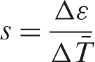
The homogeneous dilatation of measuring blocks of type 1 can be computed in terms of the sensitivity of measured strain variations to temperature variations as follows:

(2)

where Δε is the strain variation between two time instants and

Δ \bar{T}

the mean temperature variation at the same time instants. As the structural response is time delayed due to its great thermal inertia, at each time step, the current temperature has been computed as the mean value on the last six temperature measurements, corresponding to a period of 1 day and a half. A detailed explanation of this choice can be found in Ref.⁴⁰ At the generic time i, the strain is computed as:

(3)

where L_i is the current measured length of the sensor at time i and L₀ the initial length of sensors measurement base, in this case equal to 10 m for all sensors. A unique value of strain

{\bar{ε}}_{i}

(called actual strain in the following) has been used as representative of the global behavior of each measuring block; it has been considered as the true value of the axial strain and it is computed as the mean value from strains of all sensors contained in that measuring block at each measurement time. It has to be reminded that a measuring block contains only three longitudinal sensors. A filter has been applied to data to cut the temperature variations inducing strain variations lower than sensor sensitivity (2 µm m⁻¹). Sensors with persistent measurement errors have been removed from the analysis. It is useful to underline that the ratio of malfunctioning sensors for harbor structures is generally included in the range 30–50%.³⁷ Several factors can explain this relatively large amount of malfunctioning sensors: connection to the structure (electrical continuity, waterproofness, etc.), malfunctioning of the sensor itself, and global electrical continuity.

Statistical analysis on the sensitivity parameter (group 2 in Figure 5)

As previously mentioned (section ‘Steps of the analysis’), a reference situation is needed, as the data processing is performed by means of statistical analysis on data supposed as representative of the normal structural behavior under service life. Usually, the parameters representative of structural behavior are extracted by all sensor measurements during the training period in which the structure is assumed to behave normally, under the hypothesis of a spatial stationarity of the random process representing the parameters under investigation. In this application, two measuring blocks during the whole monitoring period have been considered as reference blocks to also consider potential differences due to the spatial distribution of measuring blocks. For their regular trend with time, measuring blocks C8 and B2 have been a priori assumed to have a normal behavior during the whole monitoring period.

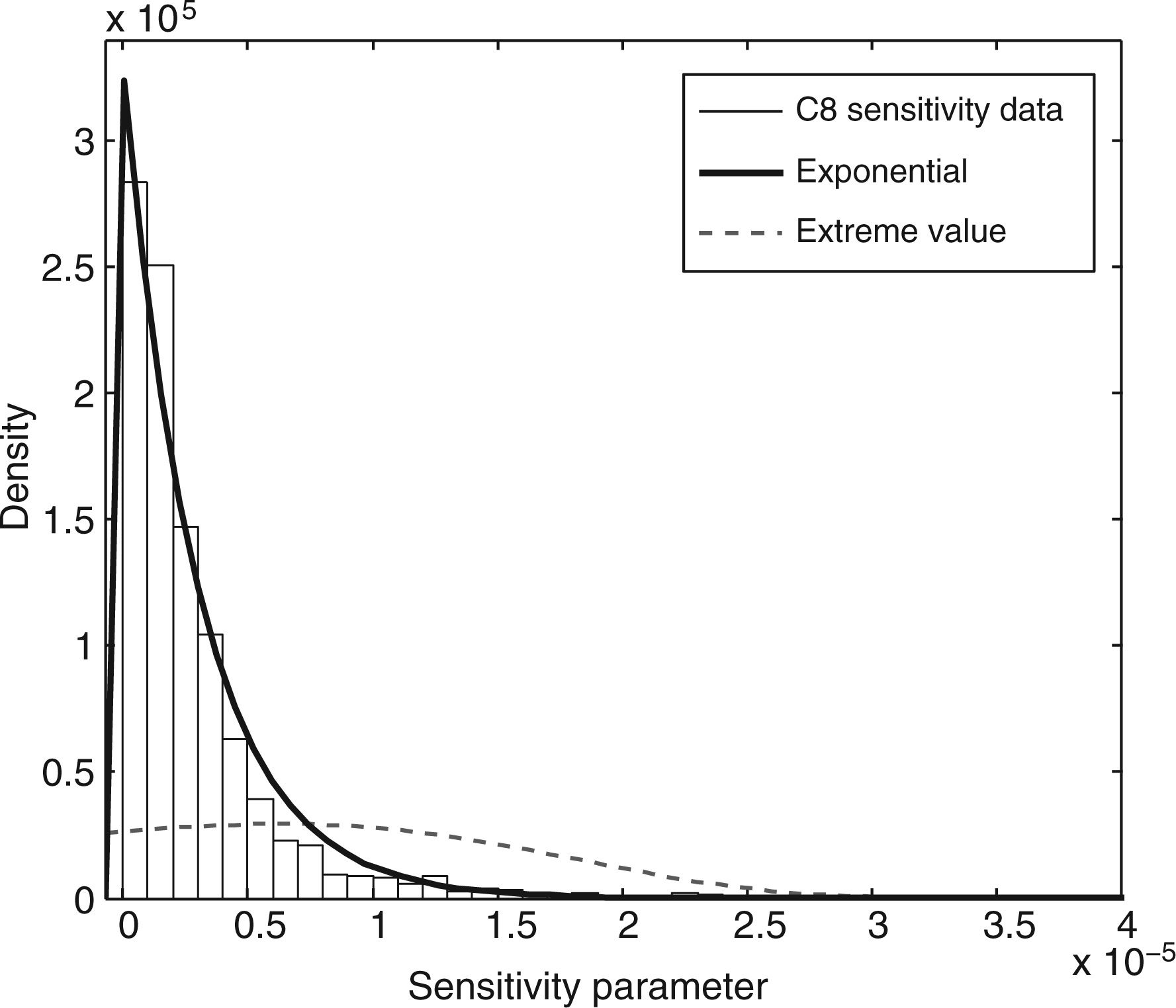
The amount of available data from the reference blocks is enough for performing a statistical analysis of the time distribution of the sensitivity parameter that is here considered as a random process indexed by the space at the measurement time. The stationarity of the random process with time has been verified by plotting the strain variation versus the temperature variation for each seasonal period (summer–winter) of the monitoring period; it can be observed that the strain variations are not related to the observation period (Figure 6). As a consequence, measurements from the reference blocks allow us to conclude that the random process is stationary with time. The sensitivity parameter has been further analyzed as a random variable of a stationary process and its probability distribution has been investigated. The estimated values of the sensitivity are well described by the exponential distribution having mean value and standard deviation 3.07 µstrain °C⁻¹ for blocks of type 1 (Figure 7).

Figure 6.

Actual strain vs temperature for reference measuring block of type 1 (C8).

Figure 7.

Probability density function of the sensitivity variable for blocks of type 1.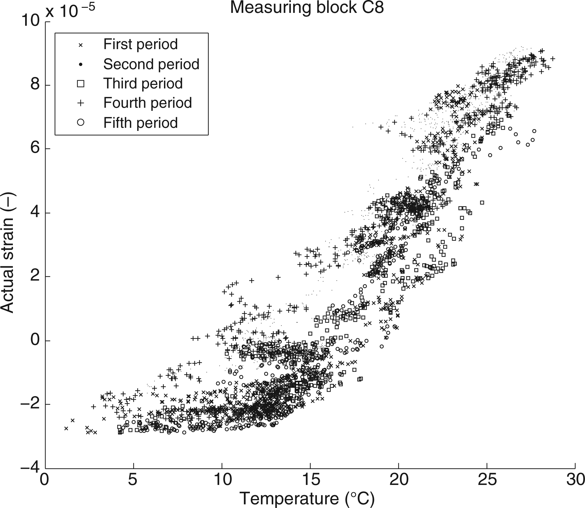

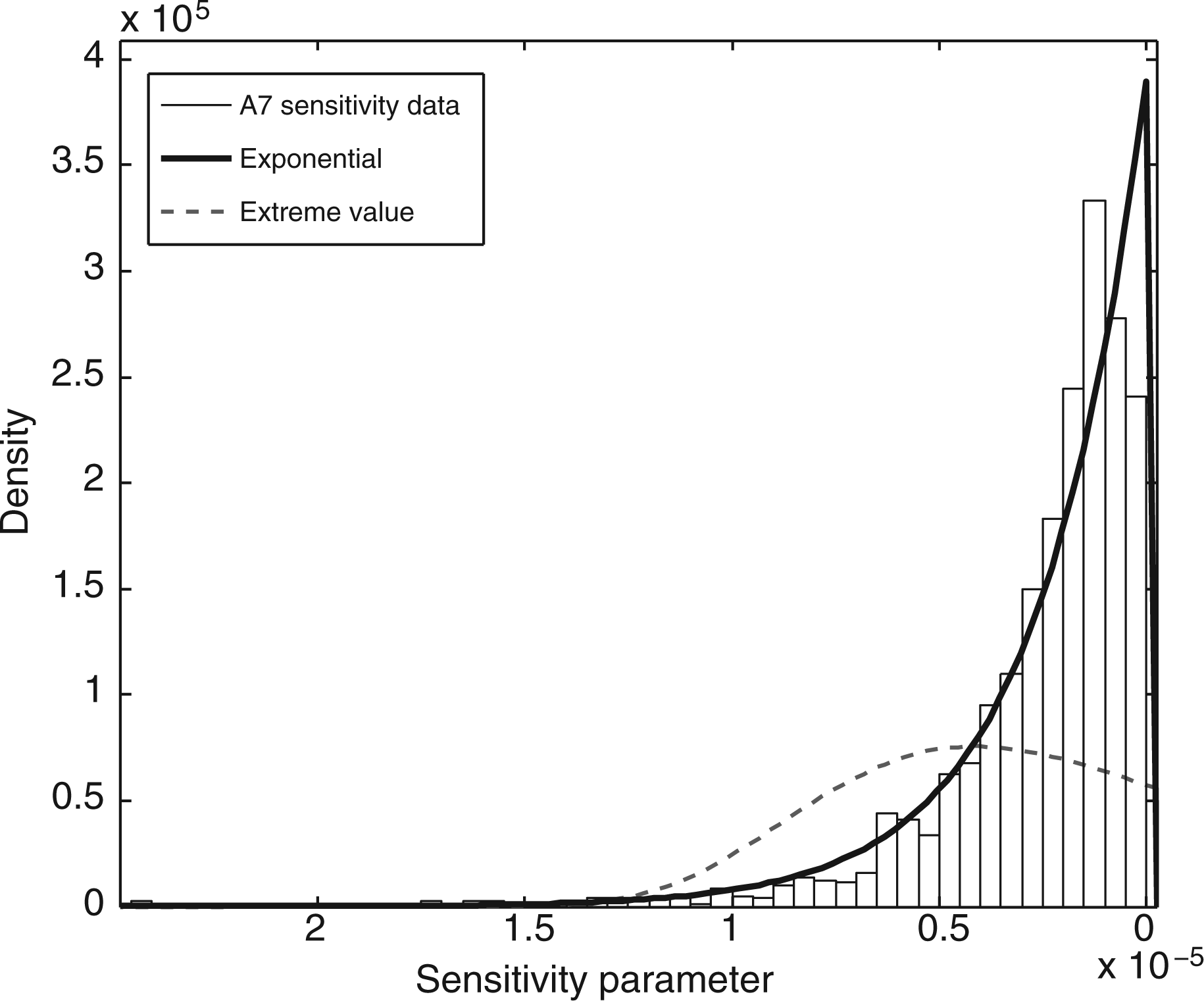
The sensitivity parameter has been also computed and plotted for measuring blocks of type 2 (Figure 8). The different data trend shown by blocks of type 1 and blocks of type 2 confirms the trend observed in the correlation indices: blocks of type 1 have a positive correlation between strain and temperature, while for blocks of type 2 the correlation is negative. Also for blocks of type 2, the estimated values of the sensitivity are well described by the exponential distribution having mean value and standard deviation −1.80 µstrain °C⁻¹ (Figure 9).

Figure 8.

Actual strain vs temperature for reference measuring block of type 2 (B2).

Figure 9.

Probability density function of the sensitivity variable for blocks of type 2.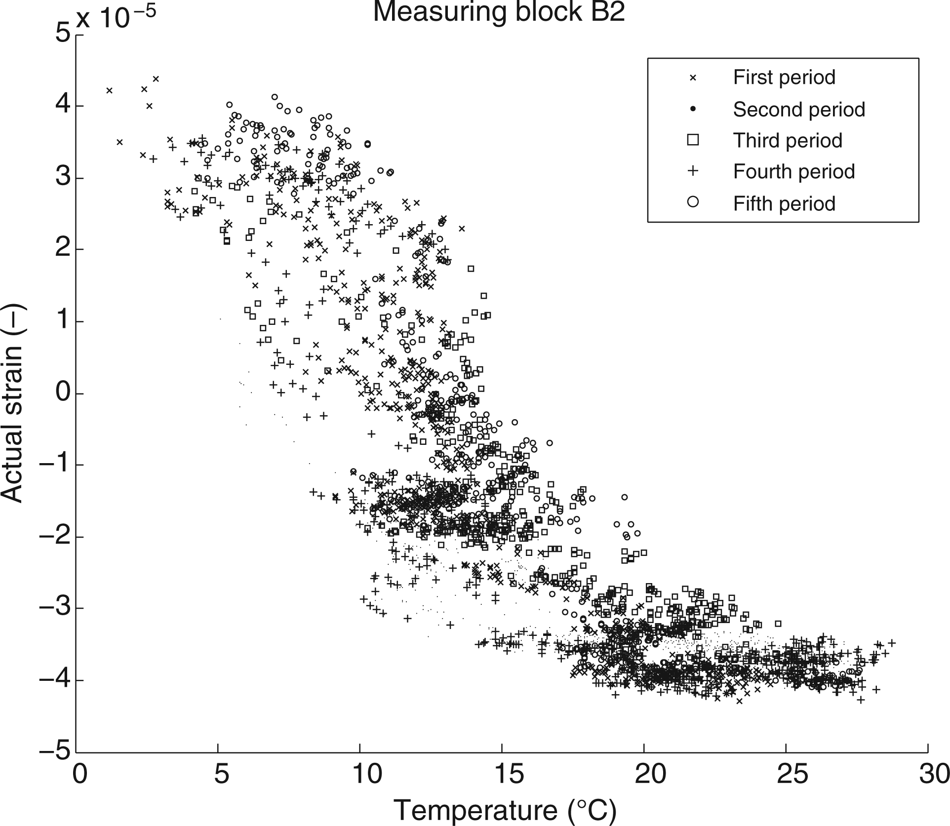

In a probabilistic framework, by considering the confidence intervals of a random variable exponentially distributed, the expected value of the sensitivity parameter for measuring blocks of type 1 is between 2.92 µstrain °C⁻¹ (μ_S(lower)) and 3.26 µstrain °C⁻¹ (μ_S(upper)) with a probability of 99%. The sensitivity parameter is considered to give a valid interpretation of the mechanical behavior of the pier. Indeed, the mean assessed value of the sensitivity parameter (between 2.9 and 3.3 µstrain °C⁻¹) is coherent but lower than the known dilatation coefficient in concrete structures (usually varying between 6 and 13 µstrain °C⁻¹ depending on the relative humidity and the aggregates). This is rightly related to the boundary conditions of the monitored crown block that is continuously supported by the lower blocks and linked to them by means of distributed vertical steel bars, so that it is not allowed to freely expand with thermal variations.

Characterization of thermal and second-order strains (group 2 in Figure 5, left)

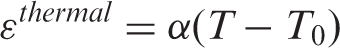
When a change in temperature occurs, the thermo-elastic strains can be written as:

(4)

where ε^thermal is the thermal strain in the linear theory and ε^{second − order} the residual strain due to non-linear effects with the temperature and other mechanical effects. The strain caused by a change in temperature from T₀ in the reference configuration (in this case the beginning of the monitoring) to T in the current configuration is called thermal strain and it can be expressed by the linear relation:

(5)

where α is here the computed sensitivity parameter.

The probabilistic analysis on the sensitivity parameter (section ‘Statistical analysis on the sensitivity parameter’) allows the assessment of the range of variation of the thermal strains for the monolithic measuring blocks given by Equation (5). For each time i:

(6)

where μ_S(lower) and μ_S(upper) are, respectively, the lower and the upper values of the sensitivity parameter associated with a probability of 99%. Consequently, it is possible to remove (filtering, Figure 5), from the strain time histories (Equation (4)), the variations due to temperature that sometimes can induce strong variations wrongly interpreted as anomalous behaviors. In this analysis, the estimated mean value of the sensitivity parameter has been used:

(7)

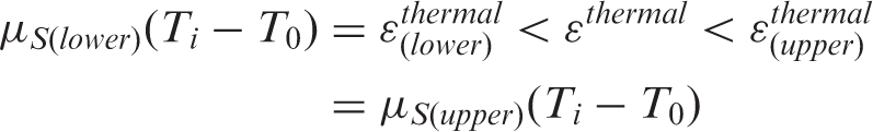
Figures 10 and 11 show the total strain and the second-order strain after removing thermal strain for block C8 (reference measuring block) and for a generic measuring block. The plots show that the second-order strains are smoother than the total ones in particular during the summer, when higher temperature variations induce greater strains. However, the second-order strains still have a cyclic and periodic behavior, probably because of secondary nonlinear effects of thermal strains with temperature variations. For their periodicity, the obtained second-order strains can be well fitted by a Fourier series, assessed by considering the data contained in the first year of measurements. The Fourier fitting, associated with its confidence intervals at 99%, also allows the validation of the classification of blocks behavior already performed with the correlation analysis in section ‘Classification of block behavior’ (Figure 5). Furthermore, the Fourier fitting gives a clearer visualization of the strain deviations in time, in terms of gradual degradation and/or instantaneous transition toward a new trend (Figure 11). The distance between the measured strains and their expected trend (and, in particular, its progression in time) can allow us to understand the possible causes of the strain deviation identified in measuring blocks of types 1A, 2A, 1B, and 2B.

Figure 10.

Second-order strain after removing thermal strain and Fourier fitting (reference measuring block). Prediction bounds are the confidence interval at 99%.

Figure 11.

Second-order strain after removing thermal strain and Fourier fitting (generic measuring block). Prediction bounds are the confidence interval at 99%.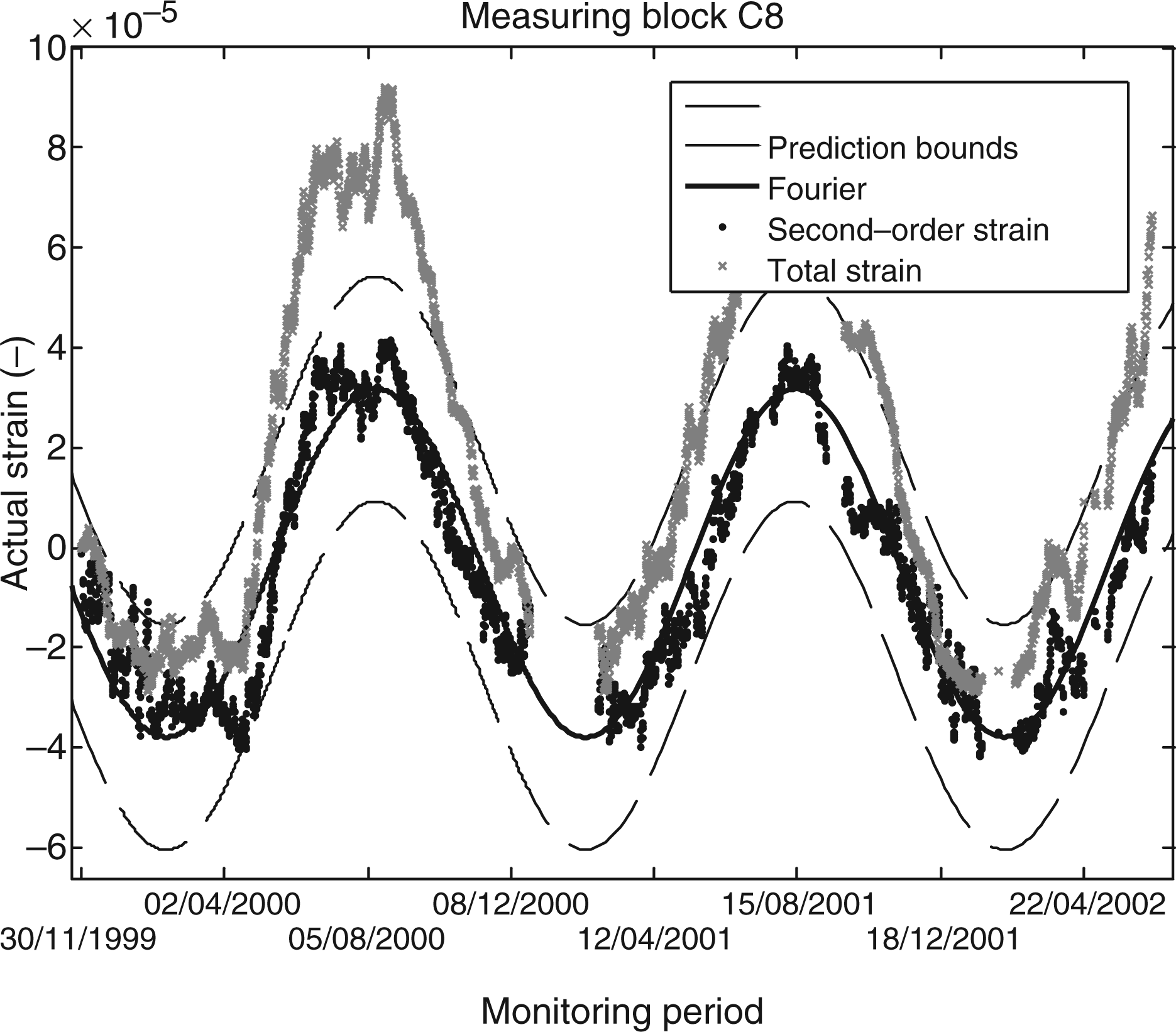

Damage-sensitive feature for blocks of type 2

Characterization of dilatation joints (group 2 in Figure 5, right)

For measuring blocks of type 2, another parameter able to describe the mechanical behavior is the variation in the joint opening Δl_j under temperature variations. This parameter can be estimated by knowing the strain measure in the block with joint (meas_j,(type2)) and assuming that the two integer blocks across the joint (block 2 on the right of the joint and block 2 on the left of the joint, Figure 1) have the same behavior of the blocks without joints.

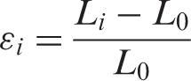
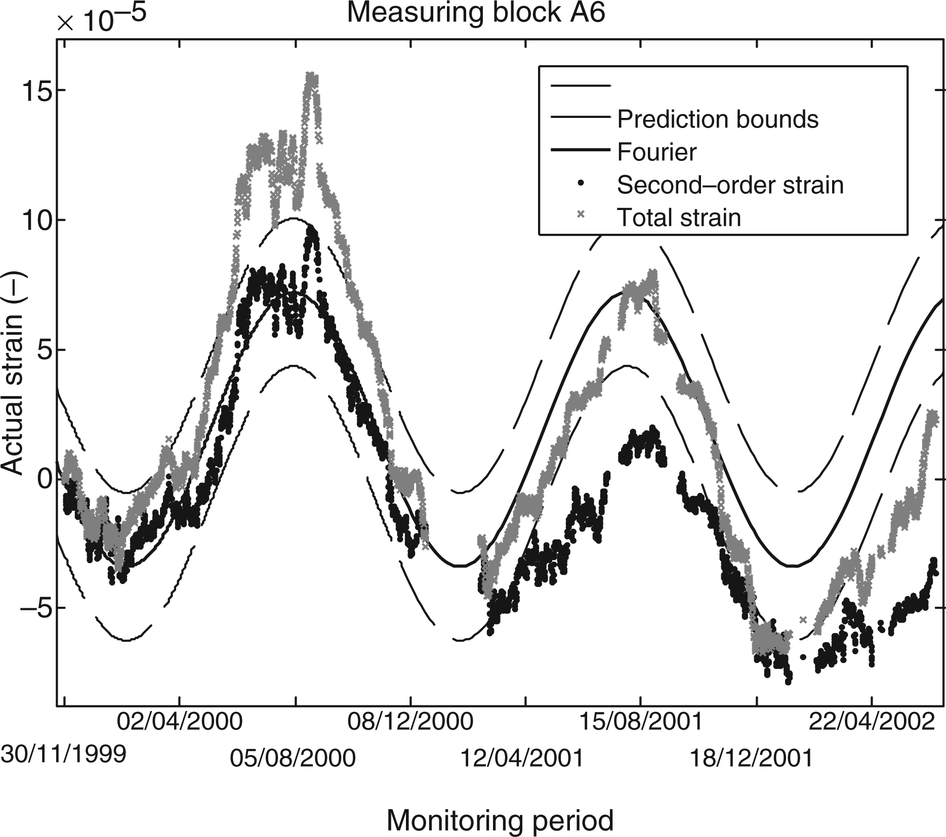
Figure 12 reports a block of type 2 in the reference state (out-of-scale) that is used as a mechanical model for the block behavior’s study. L₀ is the initial length of the block between two measurement points, in this case, 10 m. The two monolithic blocks across the joint have unknown length but the strain of the blocks of total length l* is supposed to be proportional to the strain measured in the reference measuring block of type 1; l₀ is the initial opening of the dilatation joint (unknown).

Figure 12.

Scheme of a measuring block containing a joint in the initial configuration. The ratio of n and m satisfies the following relation: 1/n + 1/m = 1, and L₀ = l₀ + l*.

Let us now consider an increase in temperature starting from this initial configuration. The block of initial length L₀ will be subjected to a shortening ΔL (as observed from measurements of blocks of type 2), while the monolithic blocks of total length l* will increase their length of Δl* as a block of type 1. As a consequence, the opening of the dilatation joint will decrease of the quantity Δl_j. These length variations satisfy the relation Δ L = Δ l_j + Δ l*.

For each measurement session j:

(8)

where

ε_{t y p e 1} = \frac{m e a s_{j (t y p e 1)}}{L_{0}}

and l* = L₀ - l₀. From the previous relations, and knowing that

Δ L = ε_{(t y p e 2)} \cdot L_{0}

, it is possible to obtain the variation in the joint opening:

(9)

where meas_j(_t_{ype 2)} is the current measurement (in mm) in a generic block of type 2. The term related to the initial opening of the joint can be neglected because

l^{*} ​ ≫ ​ l_{0}

and the relation can be simplified:

(10)

Reliability analysis

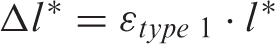
The comparison of the computed joint opening variation for the six measuring blocks of type 2 is reported in Figure 13. The plot shows that the joint opening trend is the same for all the considered blocks during the first monitoring period, with a divergence while increasing the time. The statistical analysis of the time distribution of the joint opening for the reference block B2 allows us to conclude that the joint opening variation can be also considered as a random variable of a stationary process with time (section ‘Statistical analysis on the sensitivity parameter’).

Figure 13.

Joint opening variation for blocks of type 2.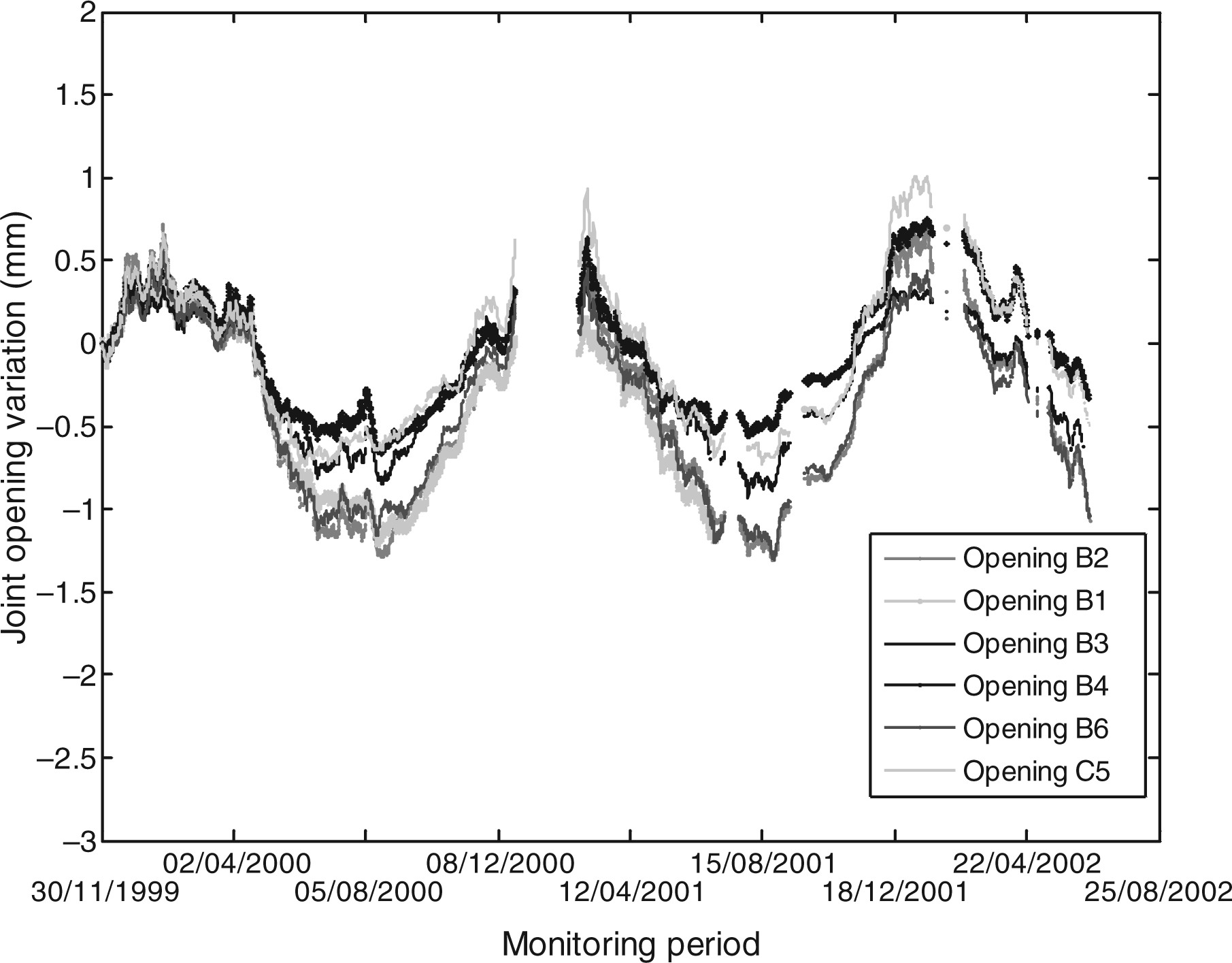

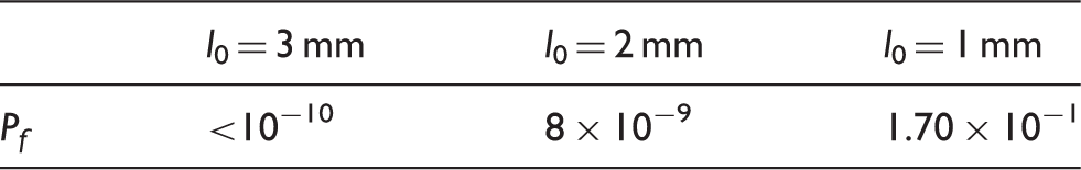
In this case, the estimated joint width values are well described by a bimodal distribution and a reliability analysis on the joint width can be performed (Figure 5). To this purpose, two samples of data have been considered: the values registered during the summer (left) and the ones measured during the winter (right). The normal distribution is able to describe the distribution of the two samples well. Figure 14 shows the probability density function for measuring blocks of type 2. The probability that the measured joint opening is lower than the initial joint opening l₀ can be computed from the fitted density functions with the aim to obtain the failure probability of the pier due to an inadequate initial joint design (limit state). With reference to Figure 14, the probability of failure can be computed as:

(11)

where the probability to have conditions like in winter or summer is related to the number of measurements in winter or summer in relation with the total number of measurements. Table 1 reports an example of the assessed failure probabilities related to different values of the initial joint opening l₀.

Figure 14.

Probability density function of the joint opening variation for blocks of type 2.

Table 1.

Failure probability due to insufficient dilatation joint width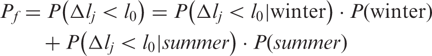

	l₀ = 3 mm	l₀ = 2 mm	l₀ = 1 mm
P_f	<10⁻¹⁰	8 × 10⁻⁹	1.70 × 10⁻¹

Damage detection (group 3 in Figure 5)

Different damage-sensitive features have been identified from previous analysis: for measuring blocks of type 1, second-order strains have been tested as sensitive damage features, while for measuring blocks of type 2, the joint opening has revealed to be a good damage indicator. The second-order strains have been used as they are not fully correlated to thermal variations and for this reason they are supposed to be more damage-sensitive than the total strains.

Different damage detection algorithms have been proposed in literature with similar data.^41,42 In this application, the linear regression analysis will be presented and successfully applied to detect the insurgence of anomalous behaviors in some measuring blocks. As regression analysis is a statistical tool for the investigation of relationships between variables,⁴³ it has been used to analyze the measuring block behavior along the pier. As demonstrated in sections ‘Statistical analysis on the sensitivity parameter’ and ‘Reliability analysis,’ the identified damage-sensitive features have been considered as random variables of a stationary process with time in reference blocks. The spatial stationarity is here assumed and the damage-sensitive features in generic measuring blocks during the training period are considered as observations of the same random variables identified for reference blocks.

Measuring blocks of type 1

A regression analysis has been performed on the second-order strain time histories by comparing the reference measuring block C8 with the other measuring blocks of type 1. The linear relationship between the reference block and the block under investigation is assessed during the reference period. The further observations of this latter block are forecasted using the linear relation previously assessed. The difference between the measured and the forecasted second-order strains (residual) gives some information on the persistency in time or on possible variations of the initial relationship. A threshold limit corresponding to a confidence interval of 99% has been evaluated taking into account the standard deviation of the residuals computed during the training period. Two different training periods have been compared: the first one considers 6 months of measurements and the second one contains the first year of measurements. The analyses have demonstrated that a training period containing at least the whole periodicity of the parameter under study (in this case the yearly cycle) is more reliable for damage detection purposes.

The plot in Figure 15 shows an example of damage detection results using the second-order strains as damage-sensitive parameter. The first subplot from the top shows the time histories of the reference measuring block (C8) and another generic block of type 1 under investigation (in this case measuring block B5). The second subplot shows the relation between the two measuring blocks strains and the regression line assessed on the basis of a training period of 1 year, with the corresponding 99% confidence interval. The training period measurements are in black points while measurements after the training period are plotted in grey crosses. The third subplot shows the time history of the residuals (absolute value) between the measured second-order strain of the block under investigation and the assessed regression line, associated with the threshold corresponding to the 99% confidence intervals. Also, in this subplot, grey crosses represent the measurements after the training period. Two anomalous overcoming phenomena of the threshold in the residual time history can be observed after the reference period, but both can be interpreted as transitory occurrences because after that the residuals get stable with time again. It can be concluded that in this measuring block no significant variations have been observed during the monitoring time.

Figure 15.

Time histories of second-order strain, regression line, and residual associated to a training period of 1 year (measuring block B5).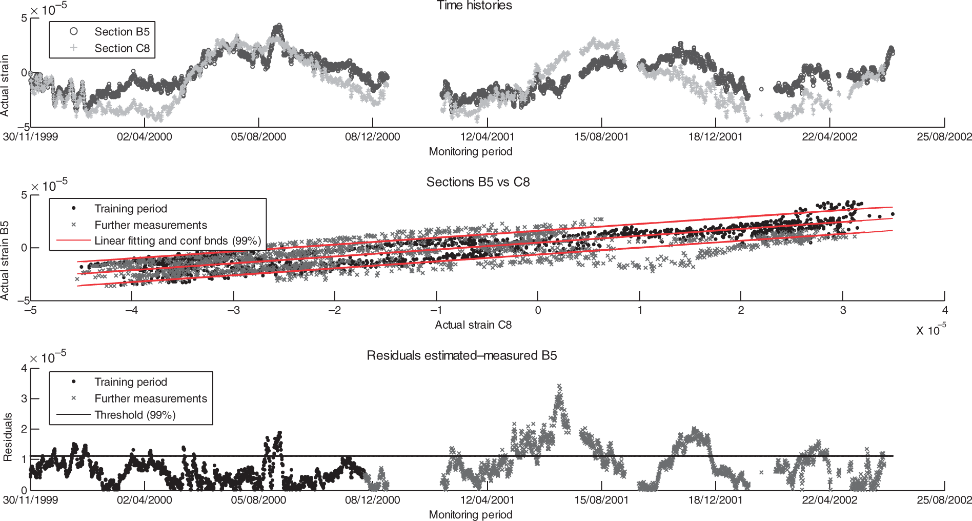

The analysis has been deepened using also the information from the correlation analysis (section ‘Classification of block behavior’). In normal conditions, the correlation index between sensors in the reference measuring block C8 and sensors in a generic measuring block of type 1 should be stationary with time under the assumption of the spatial stationarity. However, when damage or degradation occurs, correlations between sensors can change. In order to follow the strains time evolution more effectively, a window (a subset of time series) containing only a fixed number of last measurements has been used. The original aspect of this method is that the correlation index is computed only for a moving window of constant size. This means that after each measurement session, the correlation is calculated only with the measurements inside a moving window of 1 year. The use of a moving window has the advantages that it guarantees stability of average values, ensures rapid damage identification, and reduces noise effects.

Figures 16 and 17 show some examples of different sensor behaviors during the monitoring period. Plots superimpose the time histories of the residuals computed from the previous linear regression analysis (black points) and the correlation index between the second-order strains of the same pair of sensors (green line on the secondary y-axis). The time histories comparison should allow a better interpretation of the spatial evolution phenomena interesting the structure. Figure 16 reports the behavior of sensor C42. The decrease in correlation index after September 2000 is also detected by the overcoming of the threshold in the residuals. The relationship between sensors is someway changed but no other evolution in time is observed from the residual time history; this is also confirmed by the trend of the correlation index that reaches a new constant value (starting from December 2001) after a transition period related to the periodicity of the mobile window method. In this case, the detected phenomenon can be interpreted as a transition toward a new stable configuration, different from the initial one. This means that a new threshold and a new training period based on the new trend should be defined for further measurements.

Figure 16.

Residual of second-order strains, threshold associated to a training period of 1 year (line in black), and correlation index for sensors C42 and C82.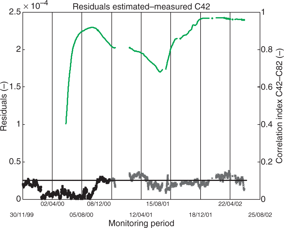

Figure 17 illustrates a typical example of a progressive phenomenon observed in sensor A62. Around April 2001, the correlation index shows a decrease and at the same time the residuals overcome the threshold. Residuals remain over the limit for all the following measurements, showing also a divergence with time, and the correlation index does not reach a new stable value. Also in this case, the periodic trend in the correlation index is related to the mobile window procedure.

Figure 17.

Residual of second-order strains, threshold associated to a training period of 1 year (line in black), and correlation index for sensors A62 and C82.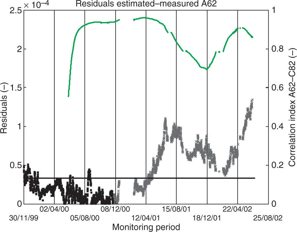

Measuring blocks of type 2

The same algorithm of linear regression analysis described in the previous section has been applied to the joint opening time histories of the reference measuring block (B2) and of a generic block of type 2 under investigation. Also in this case, a training period of 1 year has been considered. Figure 18 shows the analysis performed for the measuring block B4 that puts into evidence a degradation initiation and a gradual progression of the detected event with time.

Figure 18.

Time histories of joint opening, regression line, and residual associated to a training period of 1 year for a measuring block presenting degradation (B4).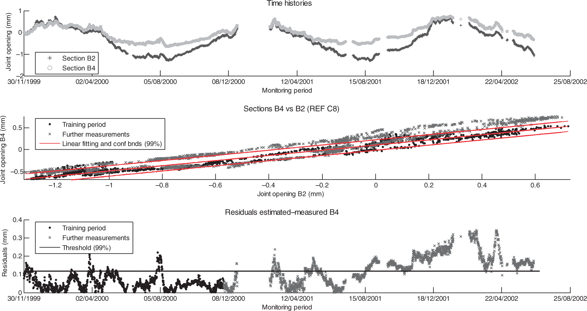

Conclusions

This article aimed at giving a general procedure for data interpretation from a continuous monitoring of complex structures. This kind of monitoring system is able to produce time-histories that have proved to be very useful for the comprehension of the structural behavior under complex interaction structure–environment. The interpretation of data from long-term static monitoring is generally faced on with different approaches, depending on the characteristics of the applications: model-based interpretation, statistical system identification, and signal processing methods for the recognition of typical response features. Some of the proposed techniques require the availability of sufficiently long and complete time-series of measurements, while the data obtained from real cases often present large incompleteness, related to system maintenance problems or malfunctioning due to various causes. In addition, if the structure has not a well-defined structural behavior and if possible variations in the structural behavior are expected to occur as a result of complex interaction phenomena, special algorithms and interpretation need to be applied.

The discussion on the complexity of data processing has been carried on by means of available data from the real long-term monitoring of a quay wall in the Port of Genoa. This example wanted to put in evidence that an optimal and unique algorithm cannot be proposed depending on the variety of applications. A multi-algorithm approach has been considered to be the best tool for understanding the structural behavior and for defining response features. This article emphasized the preliminary steps aimed at understanding the mechanical response of such a structure under operational and environmental loads. It has been discussed that the complex interaction with environmental temperature had to be taken into account too. This initial phase helped to identify typical response features that have been used for further analysis of damage identification. Due to the huge amount of instrumented blocks, in this application, the statistical analysis has proved to be successful. The extracted response features have been used as damage-sensitive parameters. The damage detection procedure has been performed using a training period during which the structure was supposed to be undamaged. Different training periods have been compared; results show that in real situations associated with high thermal variations, at least 1 year of monitoring is necessary before a damage detection procedure can be successfully applied. By the way, for harbor infrastructures, this can be considered a common lifetime if the monitoring system is installed during construction, because they undergo a long no exploitation period after construction while performing the secondary works of completion.

References

Mufti

Guidelines for structural health monitoring, design manual no. 2. Winnipeg, Manitoba. Canada: ISIS, 2001.

SAMCO. F09 report on bridge management, Final Report 2006, 2006.

Polder

Alonso

Cleland

(eds) COST 534: New materials, systems, methods and concepts for prestressed concrete structures, final report. TNO Delft: COST Office, 2009, p.388.

Del Grosso

. Monitoring of infrastructure in the marine environment (Casciati and Magonnette (eds)). In: Proceedings of the 3rd International Workshop on Structural Control – Structural Control for Civil and Infrastructure Engineering, Paris: World Scientific, 2000, pp.107–117.

Gruber

Winkler

Pressl

. Continuous monitoring in sewer networks an approach for quantification of pollution loads from CSOs into surface water bodies. Water Sci Technol 2005; 52(12): 215–223.

Yáñez-Godoy

Schoefs

Nouy

Lasne

. Reliability analysis of two in-service monitored pile-supported wharves during extreme storm loading events. In: MEDACHS 08, 1st International Conference on Construction Heritage in Coastal and Marine Environments, Lisbon, January, 2008.

Morassi

Vestroni

Dynamic methods for damage detection in structures. International Centre for Mechanical Sciences, Udine: Springer, 2009, p.221.

Catbas

Susoy

Frangopol

DM.

. Structural health monitoring and reliability estimation: long span truss bridge application with environmental monitoring data. Eng Struct 2008; 30(9): 2347–2359.

Frangopol

Strauss

Kim

. Use of monitoring extreme data for the performance prediction of structures: general approach. Eng Struct 2008; 30(12): 3644–3653.

10.

Strauss

Frangopol

Kim

. Use of monitoring extreme data for the performance prediction of structures: Bayesian updating. Eng Struct 2008; 30(12): 3654–3666.

11.

Liu

Frangopol

Kim

. Bridge safety evaluation based on monitored live load effects. J Bridge Eng 2009; 14(4): 257–269.

12.

Law

. Updating the reliability of a concrete bridge structure based on condition assessment with uncertainties. Eng Struct 2010; 32: 286–296.

13.

Moaveni

Conte

Hemez

FM.

. Uncertainty and sensitivity analysis of damage identification results obtained using finite element model updating. Comput Aided Civ Infrastruct Eng 2009; 24(5): 320–334.

14.

Morassi

. Identification of a crack in a rod based on changes in a pair of natural frequencies. J Sound Vib 2001; 242: 577–596.

15.

Caddemi

Morassi

. Crack detection in elastic beams by static measurements. Int J Solid Struct 2007; 44: 5301–5315.

16.

Lanata

. Health monitoring of concrete bridges: model simulations of prestressed beams under static environmental loading based on experimental data. In: IABMAS2010, MiniSymposia on Monitoring and Assessment of Bridges using Novel Techniques, Philadelphia, Pennsylvania, USA, July 2010.

17.

Liu

Frangopol

Kim

. Bridge system performance assessment from structural health monitoring: a case study. J Struct Eng 2009; 135(6): 733–742.

18.

Moyo

Brownjohn

JMW.

. Detection of anomalous structural behaviour using wavelet analysis. Mech Syst Sig Process 2002; 16(2–3): 429–445.

19.

Sun

Chang

CC.

. Structural damage assessment based on wavelet packet transform. J Struct Eng, ASCE 2002; 128(10): 1354–1361.

20.

Han

Ren

Sun

ZS.

. Wavelet packet based damage identification of beam structures. Int J Solid Struct 2005; 42: 6610–6627.

21.

Guo

Chen

Sun

. Experimental study of structural damage identification based on WPT and coupling. J Zhejiang Univ Sci [1009–3095] 2005; 6A(7): 663–669.

22.

Omenzetter

Brownjohn

JMW

Moyo

. Identification of unusual events in multi-channel bridge monitoring data. Mech Sys Sig Process 2004; 18: 409–430.

23.

Farrar

Lieven

NAJ

Bement

MT.

. An introduction to damage prognosis, Chapter 1. In: Inman

Farrar

Lopes

Jr Steffen

Jr (eds) Damage prognosis: for aerospace, civil and mechanical systems, 1st edn. New York: John Wiley & Sons, 2005, 1–12.

24.

Omenzetter

Brownjohn

JMW.

. Application of time series analysis for bridge health monitoring. Smart Mater Struct 2006; 15: 129–138.

25.

Nair

Kiremidjan

Law

KH.

. Time series based damage detection and localization algorithm with application to the ASCE benchmark structure. J Sound Vib 2006; 291(1): 349–368.

26.

Kraemer

Fritzen

CP.

. Sensor fault identification using autoregressive models and the mutual information concept. Key Eng Mater 2007; 347: 387–392.

27.

Wang

Ong

KCG.

. Structural damage detection using autoregressive-model-incorporating multivariate exponentially weighted moving average control chart. Eng Struct 2009; 31(5): 1265–1275.

28.

De Roeck

Peeters

Maeck

. Dynamic monitoring of civil engineering structures. In: Computational Methods for Shell and Spatial Structures, IASS-IACM, Greece, 2000.

29.

Nethal

. A review of robust regression and diagnostic procedures in linear regression. Acta Math Appl Sin 2005; 21(2): 209–224.

30.

Andersen R. Modern methods for robust regression, Sage University Paper Series on Quantitative Applications in the Social Sciences, 07-152, 2008.

31.

Tsuyoshi

Spiros

Michail

Computing correlation anomaly scores using stochastic nearest neighbors. Omaha, USA: ICDM, 2007.

32.

Deraemaeker

Reynders

De Roeck

Kullaa

. Vibration-based structural health monitoring using output-only measurements under changing environment. Mech Sys Sig Process 2008; 22: 34–56.

33.

Posenato

Lanata

Inaudi

Smith

IFC.

. Model-free data interpretation for continuous monitoring of complex structures. Adv Eng Inf 2008; 22(1): 135–144.

34.

Berry

Linoff

Mastering data mining. New York: John Wiley & Sons, 2000.

35.

Witten

Eibe

Data mining: practical machine learning tools and techniques, 2nd ed. San Francisco: Morgan Kaufmann, 2005.

36.

Del Grosso

Lanata

Brunetti

Pieracci

. Structural health monitoring of harbour piers. In: SHMII-3 2007, Vancouver, November, 2007.

37.

Yáñez-Godoy

Schoefs

Casari

. Statistical analysis of the effects of building conditions on the initial loadings of on-piles quays. Struct Health Monit 2008; 7(3): 245–263.

38.

Del Grosso

Inaudi

Lanata

. Strain and displacement monitoring of a quay wall in the port of Genoa by means of fibre optic sensors. In: 2nd European Conference on Structural Control, Paris: LNPC Press, 3–6 July, 2000, 8 pp.

39.

Glišič

Inaudi

Fibre optic methods for structural health monitoring. England: John Wiley & Sons, 2007, p.262.

40.

Lanata F. San Giorgio Pier data analysis: summary of significant results – GeM internal report (GeM-ECS-1006ins01) – June 2009, Available on-line: http://gem.ec-nantes.fr, pôle “Structures et Couplages”, équipe “Calcul des Structures”, Thème 2, 2009, 17 pp.

41.

Lanata F. Damage detection algorithms for continuous static monitoring of structures, PhD Thesis, University of Genoa, 2005.

42.

Posenato D. Model-free data interpretation for continuous monitoring of complex structures, PhD Thesis, EPFL, n. 4481, 2009.

43.

Berk

RA.

Statistical learning from a regression perspective. New York: Springer-Verlag, 2008, p.358.