Baseline-free guided wave imaging via adaptive source removal

Abstract

Structural health monitoring systems employing in situ guided wave transducers are being considered for civil, mechanical, and aerospace applications. In particular, guided wave-based imaging methods have been applied to graphically depict the area of interest and localize the damage. Most existing imaging techniques have relied on scattered waves extracted by baseline subtraction to quantify the effects of damage on the guided waves. In many cases, however, baseline data may not have been recorded or may be ineffective for baseline subtraction because of uncompensated variations between baseline and in-service signals. Proposed here is an alternative approach whereby source signals are first adaptively estimated from the in-service signals, direct arrivals are then calculated by forward propagation, and scattered signals are obtained by subtraction of the direct arrivals. Images using these scattered signals can then be created by, for example, delay-and-sum methods. This approach is demonstrated using synthetic signals generated by ray tracing and conventional delay-and-sum imaging. Its feasibility is further demonstrated with experimental data recorded on an aluminum plate using a single in situ transducer as a source and a laser vibrometer to record guided signals around the periphery of the region of interest.

Keywords

adaptive source removal baseline-free imaging dispersion correction guided waves nondestructive evaluation structural health monitoring

Introduction

Structural health monitoring (SHM) is an integrated process of nondestructively identifying the current state of a structure and providing early warning of critical structural damage.¹ Increasing efforts are being made to adopt SHM technologies as a part of aerospace, civil infrastructure, and mechanical systems to both enable condition-based maintenance and prevent catastrophic failures. One frequently considered approach to SHM of large areas is via guided elastic waves with spatially distributed arrays because such waves can interrogate a large structure with a relatively small number of transducers.^2–7

Because of the complexity of guided wave signals, many proposed SHM systems extract scattered signals from baseline data prior to performing damage detection and localization. These scattered signals, which quantify the effect of damage on the guided waves, are obtained via baseline subtraction,^8–11 where baseline signals recorded prior to damage are subtracted from the in-service signals. In many cases, however, baseline data may not have been recorded or may be unsuitable for effective baseline subtraction. For compact (e.g. circular or linear) guided wave arrays where backscattered signals are used to form images of damage, it is often unnecessary to subtract baselines if the structure is geometrically simple.^12–16 However, for the spatially distributed arrays being considered for SHM, direct arrivals from source to receiver are present in all recorded signals and, if baseline subtraction is not performed, these direct arrivals obscure small, scattered signals and prevent detection and localization of damage. Proposed here is a method whereby the direct arrivals are estimated without using baseline data and are then removed from measured signals so that small scatterers can be effectively imaged. The specific scenario considered is that of very rapidly imaging an area within which damage is suspected but no suitable baseline data are available. This situation is expected to arise when an in situ SHM system reports possible damage, and rapid follow-up inspection is desired without expensive and potentially risky disassembly. In particular, two motivating scenarios are envisioned. In the first, a noncontact method such as a scanned air-coupled transducer or a scanning laser vibrometer is used to scan the periphery of the area of interest, which is much more time efficient than raster scanning the entire area. In the second scenario, strips consisting of linear arrays of contact transducers could be placed around the periphery of the area of interest to enable rapid recording of received waves. These strips could either be permanently mounted or removable.

A number of guided wave imaging options exist for graphically depicting the area of interest. In 2004, Wang et al.³ proposed a synthetic time-reversal technique that is usually referred to as either the ellipse algorithm or delay-and-sum imaging. Pixel values are assigned based on the summation of received signals at different points in time according to the travel time from transmitter to pixel location to receiver. Several modifications have been incorporated into this technique, primarily to improve baseline subtraction prior to imaging and incorporate signal preprocessing.^10,11,17 An alternative method, referred to as the hyperbola algorithm, groups receivers in pairs with a common transmitter to obtain cross-correlation information, which provides a much larger number of contributing signals for imaging as compared to the ellipse algorithm.^7,17 Additionally, minimum variance techniques have been shown to significantly improve guided wave imaging performance^18–20 and can be applied to both the ellipse and hyperbola imaging algorithms. In this article, delay-and-sum imaging as originally proposed by Wang et al.³ is used to visualize the area of interest.

In this present study, a transducer that is permanently mounted within the area of interest is used as a transmitter (i.e., a source), and signals are recorded at multiple measurement points (or receivers) located outside of the region of interest. These points may be determined based upon access to an available surface; here they are located on the periphery of a square region. The proposed technique identifies the source location from the recorded signals, adaptively estimates the source time function, and then subtracts a propagated source time function from each recorded signal to produce estimates of the scattered signals. Scatterers that may be present in the region of interest are then imaged from these scattered signals. The uniqueness of the proposed technique is that it does not require damage-free baseline data, which may not be available for many applications of interest. The work reported here is an extension of that previously described in Ref. 21.

This article is organized as follows. The “Theory” section introduces the theoretical basis of this proposed approach. In the “Simulations” section, numerical simulation results are presented to validate the proposed techniques. The “Experiments” section contains results from experimental tests on an aluminum plate, and the article concludes in the “Conclusion” section with a summary and recommendations for future work.

Theory

Many sparse-array imaging algorithms subtract baseline data (damage-free signals) from the in-service signals to separate the relatively small scattered signals from the direct arrivals.^3,10,22 Here, however, it is assumed that baseline data are not available, which is the situation when both the region of interest and the receiver locations are determined based upon a suspected damage location that is not known a priori.

The goal of the proposed method is to image scatterers from partial wavefield data collected outside of the region of interest and without the use of baseline data. This method consists of the following steps:

Imaging with raw signals

Source location and time function estimation

Adaptive source removal

Imaging with scattered signals

After the first step of imaging with raw signals, an estimate of the source location is obtained. The source time function is estimated by back-propagating received signals to the estimated source location and averaging the results over all of the receivers. With the estimates of the source location and time function, the scattered signals can be obtained by subtracting the forward-propagated source time functions from the raw signals. Since the source signal is estimated and then forward propagated, perfect subtraction from the recorded signals is not always achieved. This is in part due to differences between nominal and actual dispersion curves of the propagation medium, differences in receiver transfer functions, and anisotropic source transmission. Therefore, an adaptive shifting and scaling algorithm is employed to adjust the propagated source signal to minimize the residual after subtraction. Finally, an image is generated using the residual signals to localize any scatterer(s). It should be noted that the two imaging steps (1 and 4) differ in two respects: (a) the data used to generate the image and (b) the assumed propagation paths. When imaging with raw signals, the propagation path is simply from each pixel location to the measurement point, whereas when imaging with scattered signals, the propagation path starts at the source location and includes the total path from source to pixel location to receiver. This entire process is for one source location; it can be applied to multiple source locations in turn to improve the performance of imaging the scatterer(s). In the following sections, the various algorithms that are a part of the above steps are described in detail.

Delay-and-sum imaging

The basic idea of conventional delay-and-sum imaging is to first delay and then sum received signals according to the calculated arrival time of a signal traveling from a transmitting transducer to one image point and on to a receiving transducer.¹⁰ For the specific case illustrated in Figure 1, pixels are imaged inside a region surrounded by receivers. 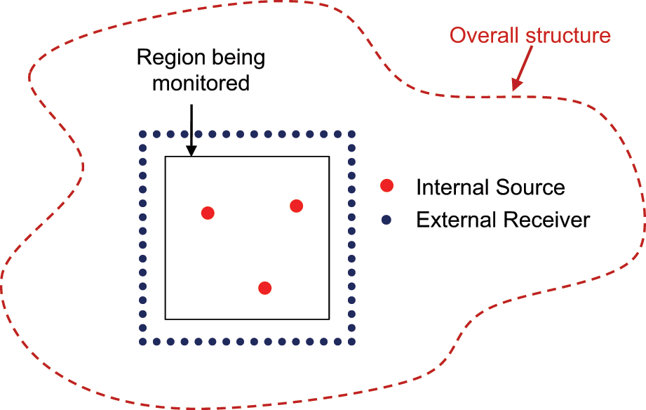To begin, consider imaging of the source, and let $z_{j} (t)$ be the sum of the delayed, or back propagated, signals for the jth pixel

Figure 1.

Illustration of the problem of imaging a region of interest using an interior source and external receivers.

z_{j} (t) = \sum_{m = 1}^{M} y_{m, j} (t)

(1)

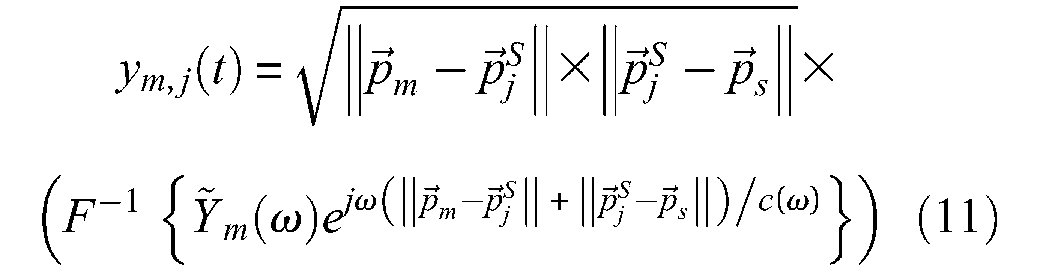
where M is the total number of receiver locations and m is the index of the receiver location. The back-propagated signals y_{m, j} (t) are given by

y_{m, j} (t) = \sqrt{‖ {\vec{p}}_{m} - {\vec{p}}_{j}^{S} ‖} y_{m} (t - Δ_{m, j})

(2)

where ${\vec{p}}_{m}$ is the position vector of the mth measurement point, ${\vec{p}}_{j}^{S}$ is the position vector of pixel j (a potential location for the source), $Δ_{m, j} = - ‖ {\vec{p}}_{m} - {\vec{p}}_{j}^{S} ‖ / c_{g}$ is the delay, and c_g is the group velocity. The initial multiplicative factor compensates for geometric spreading.

Because of the dispersive nature of Lamb waves, waves change shape as they propagate, which is not factored into the simple time shift of equation (2). There are several ways to correct for this phenomenon.^23,24 Since the back-propagation distances are known, dispersion correction as proposed in Ref. 24 is applied to modify equation (2). Using dispersion correction, the back-propagated waves in the source imaging stage are thus expressed as

y_{m, j} (t) = \sqrt{‖ {\vec{p}}_{m} - {\vec{p}}_{j}^{S} ‖} F^{- 1} {Y_{m} (ω) e^{j ω ‖ {\vec{p}}_{m} - {\vec{p}}_{j}^{S} ‖ / c (ω)}}

(3)

where $F^{- 1}$ denotes the inverse Fourier transform, Y_m(ω) is the signal y_m(t) in the frequency domain, and c(ω) is the frequency-dependent phase velocity. The magnitude of the jth image pixel, E_j, is calculated as

E_{j} = \int_{t_{1}}^{t_{2}} z_{j}^{2} (t) d t

(4)

where $z_{j} (t)$ is the sum of the back-propagated waves defined in equation (1), and t₁ and t₂ specify the time window for integration. For source estimation, t₁ = 0 and t₂ is set so that the integration window encompasses the width of the source waveform.

Source estimation

The source location ${\vec{p}}_{s}$ is estimated as the position vector corresponding to the maximum amplitude pixel in the image

s = \underset{j}{\arg max} E_{j}

(5)

The source time function is estimated as

\tilde{s} (t) = \frac{1}{M} \sum_{m = 1}^{M} y_{m, s} (t)

(6)

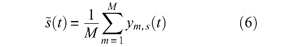
which is the average of the back-propagated signals at the estimated source location.

Adaptive source removal

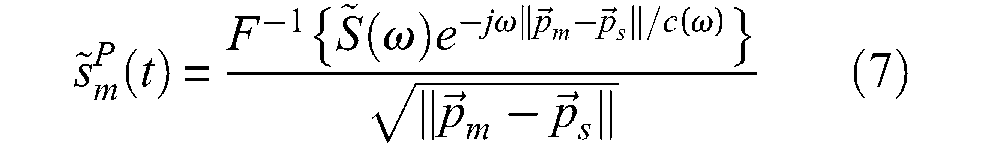
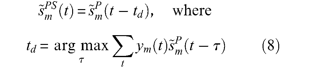
The source time function estimated in equation (6) is used to calculate the direct arrival present in each received signal, y_m(t). As previously mentioned, direct subtraction of a forward-propagated estimated source time function does not always adequately remove the direct arrival of the source. To address this issue, adaptive time-shifting and scaling is performed. The complete adaptive source removal process consists of three stages: (a) forward propagation, (b) adaptive time shifting, and (c) adaptive amplitude scaling.

To estimate the propagated source signal present in each received signal, the source time function, $\tilde{s} (t)$ , from equation (6) is forward propagated according to the distance traveled from the source to each receiver. Unlike the back propagation performed in equation (3), forward propagation shifts the source time function, $\tilde{s} (t)$ , forward (to the right), scales the signal to account for propagation loss, and reintroduces dispersion into the signal:

{\tilde{s}}_{m}^{P} (t) = \frac{F^{- 1} {\tilde{S} (ω) e^{- j ω ‖ {\vec{p}}_{m} - {\vec{p}}_{s} ‖ / c (ω)}}}{\sqrt{‖ {\vec{p}}_{m} - {\vec{p}}_{s} ‖}}

(7)

A time shift t_d that aligns ${\tilde{s}}_{m}^{P} (t)$ and $y_{m} (t)$ is obtained through finding the maximum cross-correlation value

{\tilde{s}}_{m}^{PS} (t) = {\tilde{s}}_{m}^{P} (t - t_{d}), where t_{d} = \underset{τ}{\arg max} \sum_{t} y_{m} (t) {\tilde{s}}_{m}^{P} (t - τ)

(8)

Finally, the propagated source signal is scaled to best match the received data

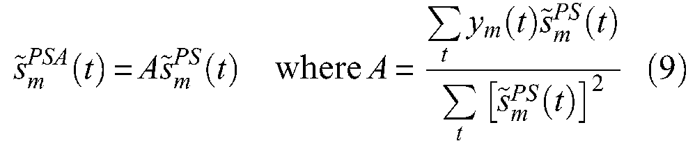
{\tilde{s}}_{m}^{PSA} (t) = A {\tilde{s}}_{m}^{PS} (t) where A = \frac{\sum_{t} y_{m} (t) {\tilde{s}}_{m}^{PS} (t)}{\sum_{t} {[{\tilde{s}}_{m}^{PS} (t)]}^{2}}

(9)

Note that the superscript “PSA” denotes the combined forward propagation, time shift, and amplitude scaling, respectively. An estimate of the scattered signal is obtained by subtracting the propagated, shifted, and scaled source signal

{\tilde{y}}_{m} (t) = y_{m} (t) - {\tilde{s}}_{m}^{PSA} (t)

(10)

These are the signals that are used to image any scatterers. Note that if there is a defect directly in line between the source and receiver, its primary effect will be to attenuate and possibly time shift the direct arrival (i.e., forward scattering). Thus, the proposed adaptive source removal process could suppress the signal scattered from such a defect. However, since there are multiple receivers, scattered signals will not be suppressed from most of the received signals, and effective imaging of damage can still take place.

Imaging with scattered signals

The same delay-and-sum imaging method described in the section “Delay-and-sum imaging” is applied to the imaging of scatterers with appropriate modifications to the delay law and integration window. The back-propagation path for the scattered waves consists of two parts: (a) the path from the receiver to the pixel location (a potential location for the scatterer) and (b) the path from the pixel location to the source location. Therefore, the back-propagated waves in equation (1) are given by

y_{m, j} (t) = \sqrt{‖ {\vec{p}}_{m} - {\vec{p}}_{j}^{S} ‖ \times ‖ {\vec{p}}_{j}^{S} - {\vec{p}}_{s} ‖} \times (F^{- 1} {{\tilde{Y}}_{m} (ω) e^{j ω (‖ {\vec{p}}_{m} - {\vec{p}}_{j}^{S} ‖ + ‖ {\vec{p}}_{j}^{S} - {\vec{p}}_{s} ‖) / c (ω)}})

(11)

The integration window in equation (4) is reduced to a single point by setting t₁ and t₂ to the time of the maximum amplitude of the estimated source time function. This “instantaneous windowing” has been shown to significantly reduce imaging artifacts.²⁰

Simulations

Simulation setup

Guided waves that are excited by a single-mode point source in a 2400-mm × 1500-mm × 3.18-mm aluminum plate are simulated by ray tracing with dispersion and geometric spreading. The receivers, or measurement points, are evenly distributed around the perimeter of a 600-mm × 600-mm square with a spacing of 24 mm, for a total of 96 receivers. As illustrated in Figure 2 for a smaller number of measurement points, a single source and a single scatterer are considered, and the region of interest is in the center of the plate. The source is modeled as an isotropic emitter of A₀ waves with a source time function of a 40-kHz, four-cycle, Hanning-windowed sinusoid. Note that 40 kHz was selected for the simulations to match experiments because the best guided wave mode purity was achieved at this frequency. The scatterer is modeled as a perfectly uniform point scatterer with a scattering coefficient of 0.05, which was determined to be a reasonable match to experimental data. For each receiver location, the received signal is modeled as a sum of the direct arrival of the source wave, the first scattered arrival, and the first edge reflections from the top and bottom edges of the plate. Each echo (direct or scattered) is dispersed using the nominal A₀ dispersion curve for the plate of interest over the appropriate propagation path. Amplitude scaling inversely proportional to the square root of the propagation distance for the direct arrival and first edge reflections is also applied to account for geometric spreading. For the scattered waves, scaling inversely proportional to the square root of the product of the two propagation distances (source-to-scatterer and scatterer-to-receiver) is applied.

Figure 2.

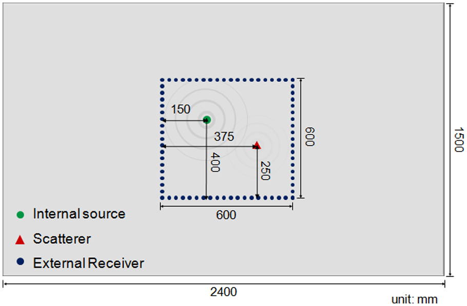
Diagram of a 2400-mm × 1500-mm × 3.18-mm-thick 6061 aluminum plate with a centered region of interest that is 600 mm × 600 mm. The single internal source, multiple external receivers, and the single scatterer are shown.

Results

Figure 3 shows typical signals at two representative receiver locations, one where the direct arrival and scattered waves are well separated, and the other where they are overlapped. The four signals shown are (1) simulated measured signals, (2) forward-propagated signals of the source time function estimated from the back-propagated signals, (3) residuals between the measured signals and the forward-propagated signals with a simple subtraction, and (4) residuals with adaptive source removal. As can be seen in the bottom plot of Figure 3(b), adaptive source removal does suppress the scattered wave for the case where the direct arrival and the scattered echo overlap.

Figure 3.

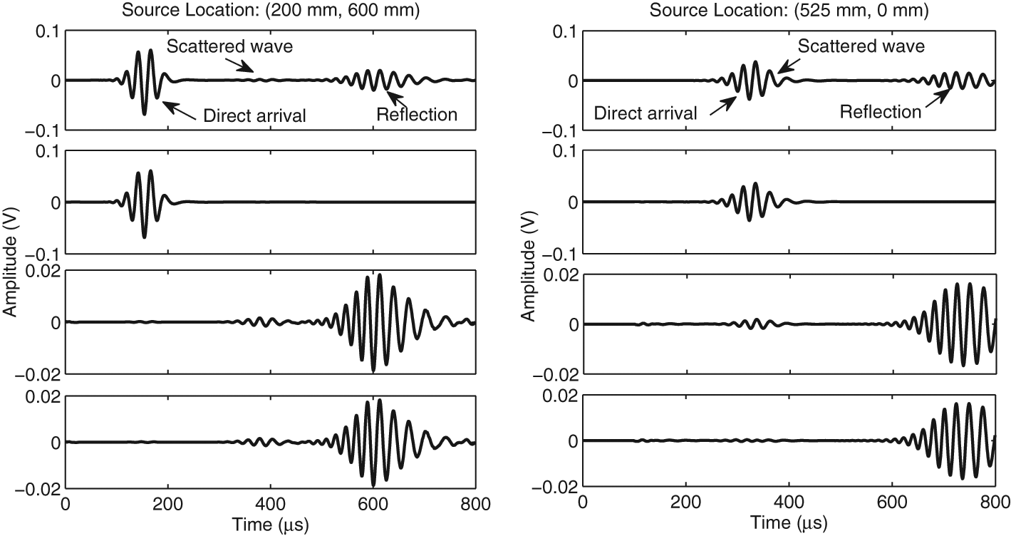
Simulated measured signals, forward-propagated signals, residuals with simple subtraction, and residuals with adaptive source removal from two representative receiver locations, where the (x, y) coordinates are shown for each signal: (a) direct arrival and scattered waves are well separated and (b) direct arrival and scattered waves are overlapped.

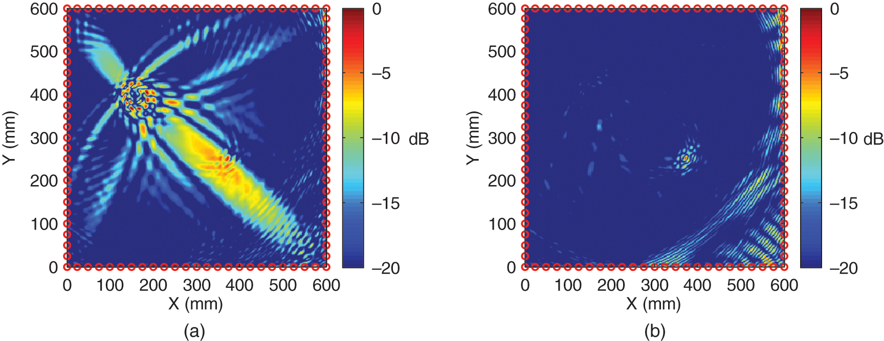
As previously described, each received signal is back propagated according to the appropriate delay law and summed with the other back-propagated signals to estimate the source time function. At the pixel location corresponding to the source location, all of the back-propagated signals are expected to be aligned in time and have very similar shapes. Figure 4(a) shows the delay-and-sum image of the source constructed using the 96 receivers. In this and subsequent images, the receiver locations are denoted by open circles around the periphery, and the pixel resolution of the image is 2 mm. It can be seen from this image that the source location can be readily determined from the location of the maximum amplitude pixel. The source time function is obtained as per equation (6) using the dispersion-corrected and back-propagated signals of equation (3).

Figure 4.

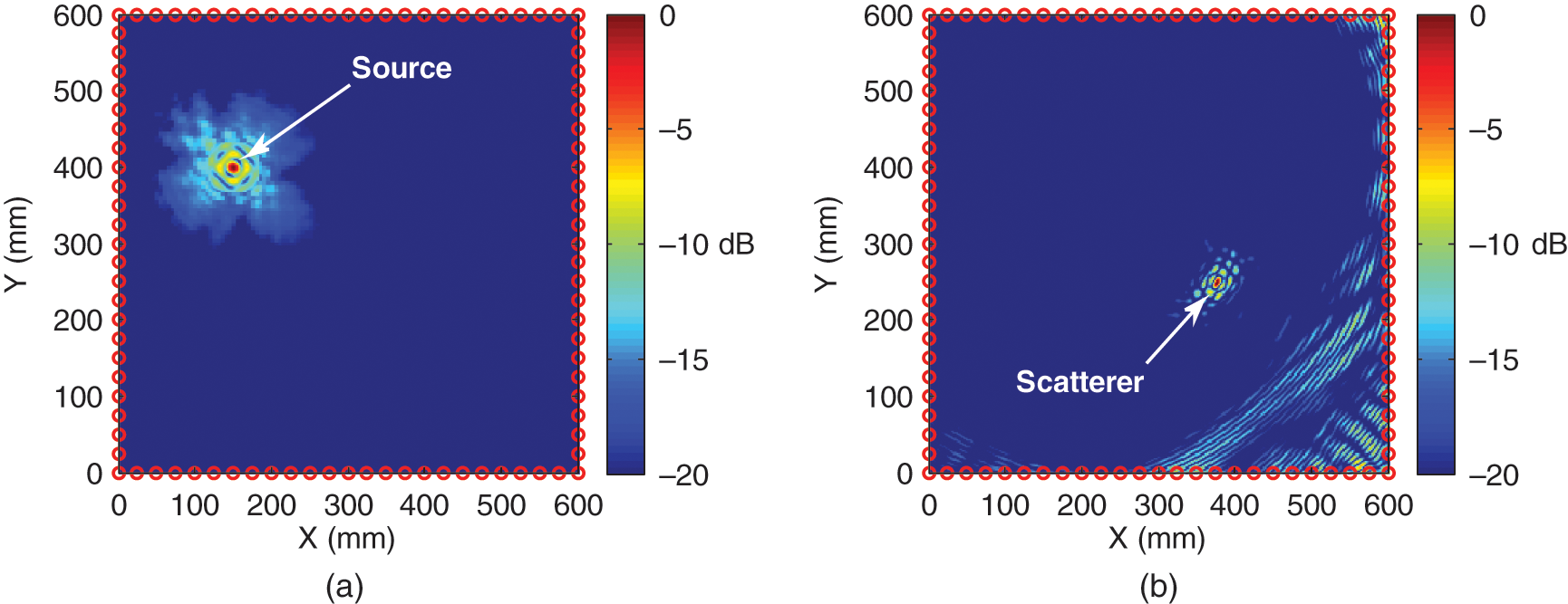
Images constructed from simulated signals: (a) delay-and-sum image of the source constructed from the raw data and (b) delay-and-sum image of the scatterer constructed from signals with direct arrivals removed via adaptive source removal. Each image is shown on a 20-dB scale normalized by its maximum pixel value, and the circles around the periphery indicate the receiver locations.

Then, the estimated source time function is forward propagated and subtracted from the measured signals prior to imaging. The bottom plots in Figure 3 show example residual signals after adaptive source removal. Figure 4(b) shows the image that is constructed using these residual signals. The source that was dominant in Figure 4(a) is essentially completely removed, and the scatterer is now clearly visible. The artifacts in the lower right corner of Figure 4(b) are caused by edge reflections, which are not reduced by the source removal process. The patterns around both the source and the scatterer in Figure 4(a) and Figure 4(b) are due to constructive and destructive inference of the summed signals and cannot be removed by, for example, imaging with the analytic signals.

Imaging with and without adaptive source removal

Imaging of the scatterer was repeated using slightly inaccurate dispersion information to demonstrate the efficacy of the proposed adaptive source removal. During both the back-propagation and forward-propagation steps, dispersion curves were utilized that had been calculated using bulk wave speeds and a plate thickness that were 5% less than their nominal values (i.e., those used to calculate the simulated signals). Figure 5(a) shows the image constructed without adaptive source removal (i.e., simple subtraction of the source). Resulting imaging artifacts are very large, and the scatterer can no longer be located. Figure 5(b) shows the corresponding image after adaptive source removal, and it can be seen that imaging artifacts are significantly smaller, permitting the scatterer to be unambiguously located. Note that the source estimation step is identical for the two images; the only difference is the source removal step. A comparison to Figure 4(b) indicates that the imaging artifacts in the bottom right corner are caused by the edge reflections. Ongoing efforts are underway to remove edge reflections and further minimize imaging artifacts.²⁵

Figure 5.

Delay-and-sum images of the scatterer constructed from simulated signals using slightly erroneous dispersion curves: (a) direct arrivals removed via simple subtraction and (b) direct arrivals removed using the adaptive source removal algorithm.

Experiments

Experimental setup

Experiments were performed on a 6061 aluminum plate with dimensions of 2400 mm × 1500 mm × 3.18 mm. A 19.05-mm-diameter lead zirconate titanate (PZT) transducer was glued to the plate and used as a source of A₀ waves, and a 12.7-mm-diameter cylindrical steel rod 100 mm long was also glued to the plate and served as the scatterer. All dimensions are identical to those shown in Figure 2 for the simulations, and photographs of both sides of the plate are shown in Figure 6. A Polytec PSV400M2 scanning laser Doppler vibrometer (SLDV) was utilized to scan the boundary of a 600-mm × 600-mm square region that was located in approximately the center of the plate as shown in Figure 6(b). The PZT transducer was excited with a 40 kHz, four-cycle, Hanning-windowed tone burst to generate A₀ mode Lamb waves. Data were collected at 92 measurement points evenly spaced on the square periphery, resulting in a spatial increment of approximately26 mm.

Figure 6.

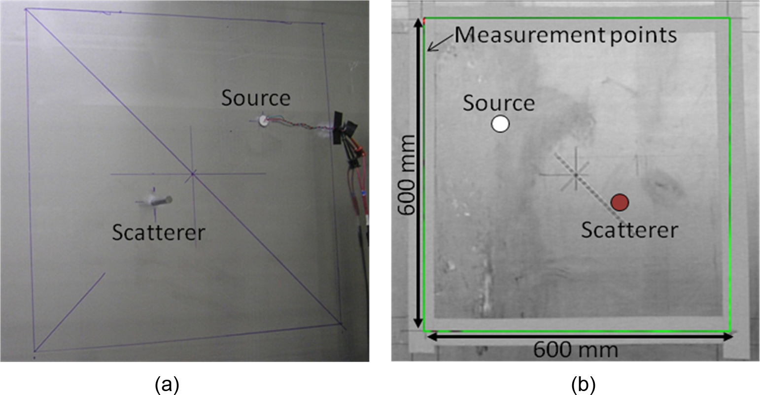
Photographs of the experimental setup: (a) PZT transmitter and metal rod scatterer glued on the back side of the plate and (b) the boundary of a 600-mm × 600-mm square region for wavefield measurements on the front side of the plate.

Results

The same algorithm and imaging resolution as previously described for the simulations were applied to the experimental data to first image the source and then the scatterer. Figure 7 shows typical signals at two different measurement points, which are close to the locations shown in Figure 3 for simulated signals. The residuals in Figure 7 show the necessity of adaptive source removal because there are inevitably errors in dispersion information caused by the difficulty of accurately knowing material properties and the specimen thickness.

Figure 7.

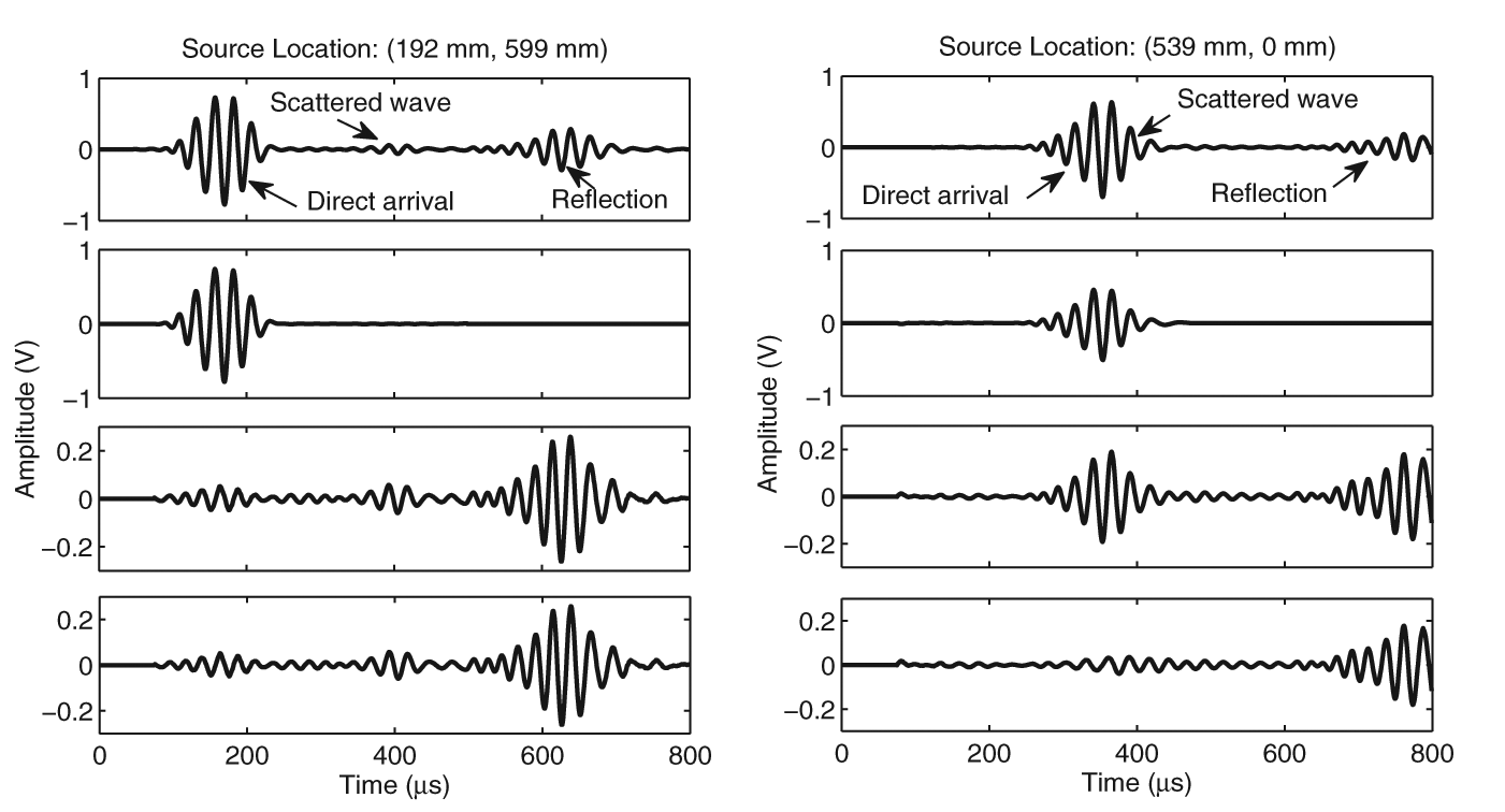
Experimentally measured signals, forward-propagated signals, residuals with simple subtraction, and residuals with adaptive source removal from two representative receiver locations: (a) direct arrival and scattered waves are well separated and (b) direct arrival and scattered waves are overlapped.

Similar to Figure 4, Figure 8 shows images of the source and the scatterer. Note that in Figure 8(b), there are essentially no visible source-related artifacts because of the effectiveness of adaptive source removal, and the scatterer is unambiguously identified. The actual scatterer (i.e., the steel rod) was located at (375 mm and 250 mm) from the lower left corner of the area of interest as shown in Figure 2, and the maximum pixel value was obtained at (370 mm and 256 mm). If Figure 8(b) is compared to Figure 4(b), which is the corresponding image from the simulated data, it is clear that the image of the scatterer for the experimental data is significantly larger in spatial extent. However, a comparison of the source time functions for the two cases indicates that the experimental source time function is longer in duration. Both images show a strong periodic pattern in the immediate vicinity of the scatterer, which is more pronounced for the longer duration source time function. As explained previously, these patterns are caused by constructive and destructive interferences of the back-propagated scattered signals during the signal summation process.

Figure 8.

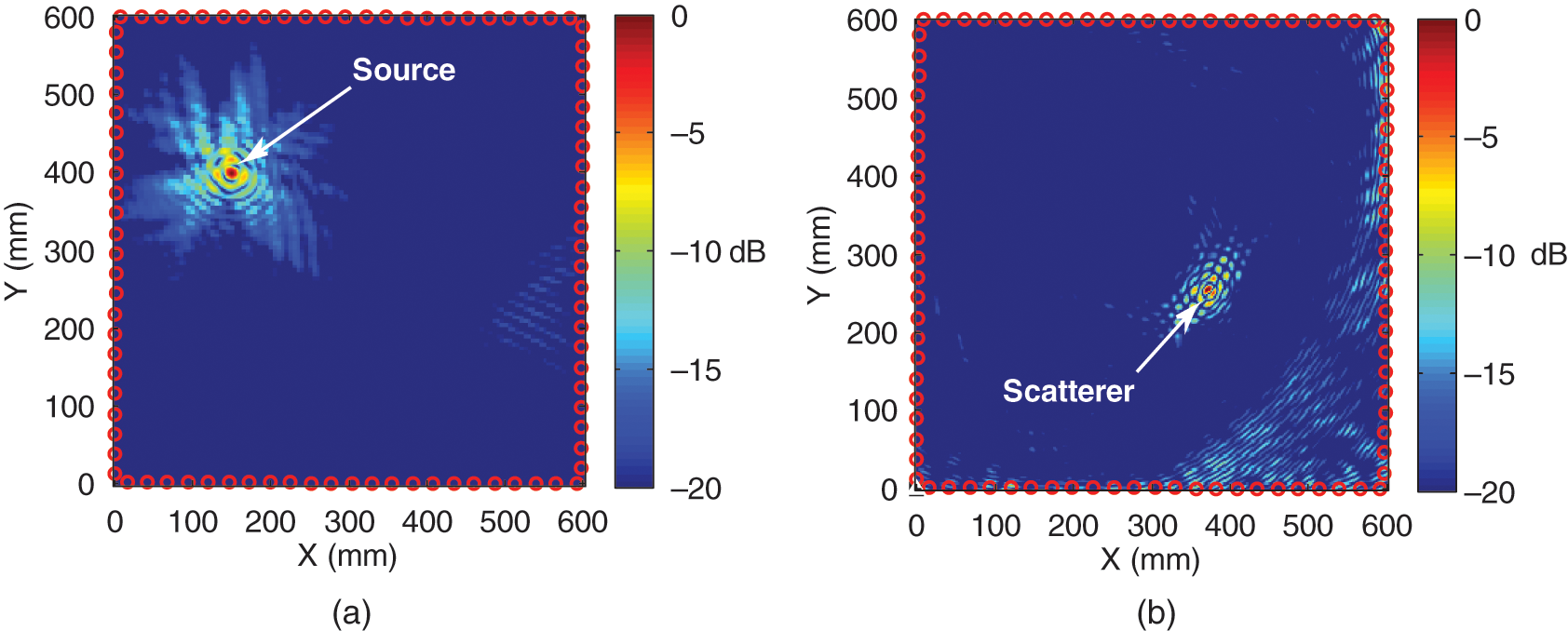
Images constructed from experimental data: (a) delay-and-sum image of the source constructed from the raw data and (b) delay-and-sum image of the scatterer constructed from signals with direct arrivals removed via adaptive source removal. Each image is shown on a 20-dB scale normalized by its maximum pixel value, and the circles around the periphery indicate the receiver locations.

For both simulated and experimental data, the scatterer can be clearly identified in the final image. Although there are some artifacts in both images caused by edge reflections, the magnitude of the imaged scatterer enables unambiguous detection of the scatterer despite the fact that the scattered waves are much smaller in amplitude than the edge reflections as shown in the top plots of Figure 7.

Variable configurations of measurement points

The configuration of measurement points was varied to investigate its effect on the imaging results. Figure 9 shows images obtained using four different configurations of measurement points: (a) left-side-only measurements, (b) right-side-only measurements, (c) left-and-right-side measurements, and (d) top-and-bottom measurements. A comparison of Figure 9(a) and Figure 9(b) shows the detrimental effect of overlapping direct and scattered signals. In Figure 9(a), the receiver locations are such that the scatterer is not located on or near any of the source–receiver paths, which means that the direct and scattered arrivals are well separated in time. Thus, adaptive source removal is very effective and the scatterer is well localized. In contrast, the receivers of Figure 9(b) are very unfavorably located with the scatterer located on or near most of the source–receiver direct paths. The resulting overlapping echoes cause the source removal process to be ineffective by suppressing most of the scattered signals from the adaptive source removal, and the resulting image quality is very poor. It is also interesting to note that the artifacts of Figure 9(c) and Figure 9(d) are different, which suggests that different combinations of receivers may perform better than others depending upon the actual locations of source(s), scatterer(s) and boundaries.

Figure 9.

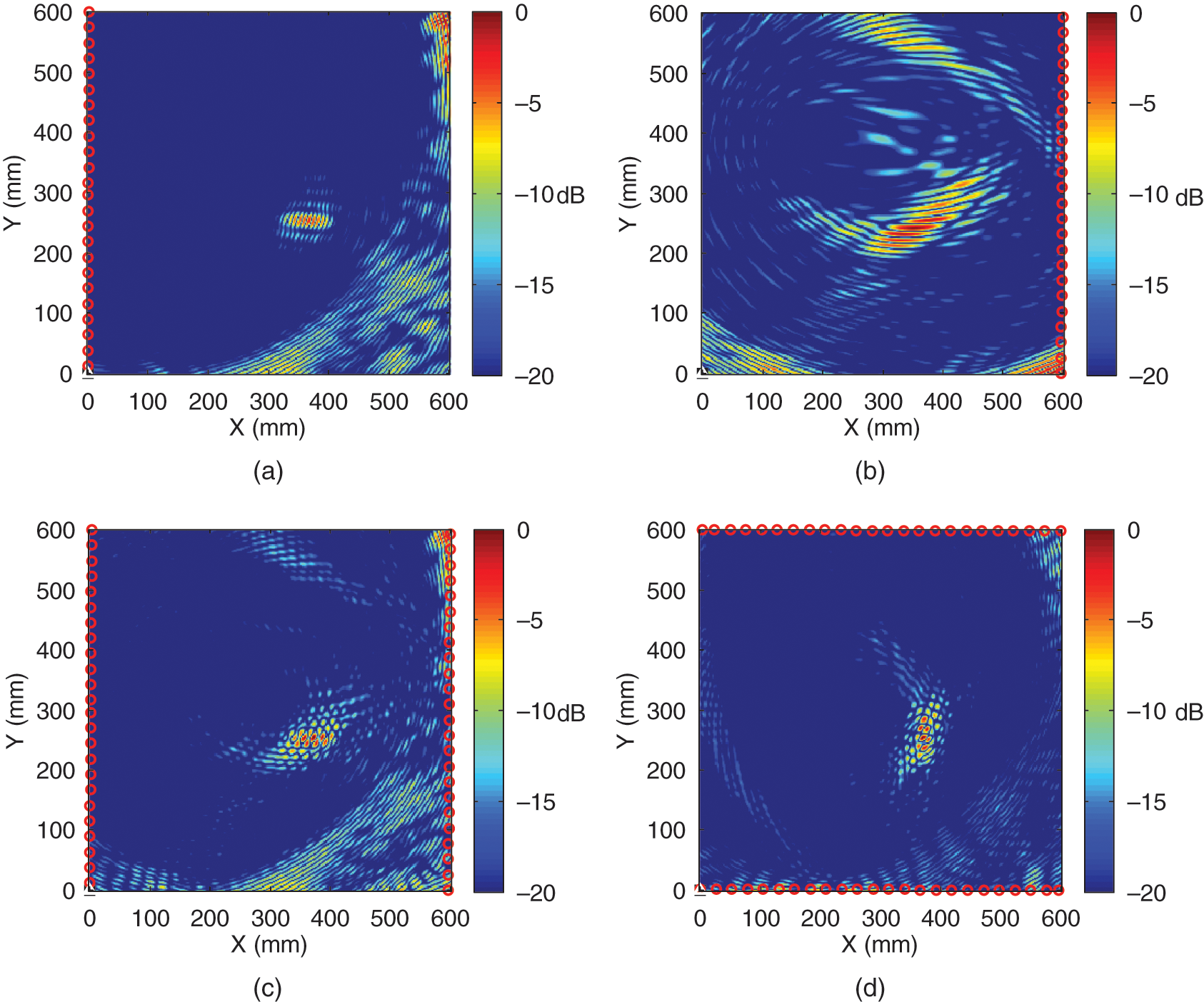
Images of the scatterer constructed from experimental data using various configurations of measurement points: (a) image from one left-side measurement with 24 points, (b) image from one right-side measurement with 24 points, (c) image from left-and-right-side measurements with 48 points, and (d) image from top-and-bottom measurements with 48 points.

Conclusion

This article presents a baseline-free method for imaging scatterers within a region of interest, and was demonstrated using an interior source and signals recorded on the boundary of the region. Both simulations and experiments show that a small scatterer can be successfully imaged without the use of any baseline information. Dispersion correction and adaptive source removal are integral to the success of imaging method. This method is applicable to imaging of structural damage in inaccessible regions that are being monitored with permanently attached transducers, and could also be applied to many other source–receiver configurations for both SHM and nondestructive evaluation.

The present study is limited to a single scatterer in a simple plate with limited edge reflections; that is, the edge reflections have minimal overlap with scattered echoes. It is recommended that future work addresses more complicated structural configurations that give rise to scattering from geometrical features. Utilization of multiple sources, which is straightforward, should provide more robustness to the additional echoes that arise from increased structural complexity. Adaptive imaging and in situ estimation of dispersion are additional techniques that could be considered to improve imaging performance.

Footnotes

Funding

This work is supported by the Air Force Office of Scientific Research (AFOSR), Structural Mechanics Division, Grant No. FA9550-08-1-0241, and the NASA Graduate Student Research Program (GSRP), Grant No. NNX08AY93H.

References

Adams

. Health monitoring of structural materials and components: methods with applications. West Sussex: John Wiley & Sons, 2007.

Michaels

. Sparse ultrasonic transducer array for structural health monitoring. In: Review of progress in QNDE (eds Thompson

Chimenti

), vol. 23B, 2004, pp.1476–1483. New York: American Institute of Physics.

Wang

Rose

Chang

F-K

. A synthetic time-reversal imaging method for structural health monitoring. Smart Mater Struct 2004; 13(2): 415–423.

. Crack identification in aluminium plates using Lamb wave signals of a PZT sensor network. Smart Mater Struct 2006; 15(3): 839–849.

Michaels

. Guided wave signal processing and image fusion for in situ damage localization in plates. Wave Motion 2007; 44(6): 482–492.

Zhao

Gao

Zhang

. Active health monitoring of an aircraft wing with embedded piezoelectric sensor/actuator network. I. Defect detection, localization and growth monitoring. Smart Mater Struct 2007; 16(4): 1208–1217.

Croxford

Wilcox

Drinkwater

. Guided wave SHM with a distributed sensor network. In: Proceedings of the SPIE, vol. 6935. Bellingham, WA: SPIE, 2008, pp.69350E-1–69350E-9.

Michaels

. A methodology for structural health monitoring with diffuse ultrasonic waves in the presence of temperature variations. Ultrasonics 2005; 43(9): 717–731.

Konstantinidis

Drinkwater

Wilcox

. The temperature stability of guided wave structural health monitoring systems. Smart Mater Struct 2006; 15(4): 967–976.

10.

Michaels

. Detection, localization and characterization of damage in plates with an in situ array of spatially distributed ultrasonic sensors. Smart Mater Struct 2008; 17(3), 035035 (15pp).

11.

Clarke

Cawley

Wilcox

. Evaluation of the damage detection capability of a sparse-array guided wave SHM system applied to a complex structure under varying thermal conditions. IEEE Trans Ultrason Ferroelectr Freq Control 2009; 56(12): 2666–2678.

12.

Wilcox

. Omni-directional guided wave transducer arrays for the rapid inspection of large areas of plate structures. IEEE Trans Ultrason Ferroelectr Freq Control 2003; 50(6): 699–709.

13.

Purekar

Pines

Sundararaman

. Directional piezoelectric phased array filters for detecting damage in isotropic plates. Smart Mater Struct 2004; 13(4): 838–850.

14.

Rajagopalan

Balasubramaniam

Krishnamurthy

. A single transmitter multi-receiver (STMR) PZT array for guided ultrasonic wave based structural health monitoring of large isotropic plate structures. Smart Mater Struct 2006; 15(5): 1190–1196.

15.

Olson

DeSimio

Derriso

. Beam forming of Lamb waves for structural health monitoring. J Vib Acoust 2007; 129(6): 730–738.

16.

Giurgiutiu

. In situ 2-D piezoelectric wafer active sensors arrays for guided wave damage detection. Ultrasonics 2008; 48(2): 117–134.

17.

Michaels

Croxford

Wilcox

. Imaging algorithms for locating damage via in situ ultrasonic sensors. In: Proceedings of IEEE sensors applications symposium, Piscataway, NJ: IEEE, 2008, pp.63–67.

18.

Michaels

Hall

Hickman

. Sparse array imaging of change-detected ultrasonic signals by minimum variance processing. In: Review of progress in QNDE (eds Thompson

Chimenti

), vol. 28A1, 2009, pp.642–649. New York: American Institute of Physics.

19.

Michaels

Hall

Michaels

. Adaptive imaging of damage from changes in guided wave signals recorded from spatially distributed arrays. In: Proceedings of SPIE, vol. 7295. Bellingham, WA: SPIE, 2009, pp.729515-1–729515-11.

20.

Hall

Michaels

. Minimum variance ultrasonic imaging applied to an in situ sparse guided wave array. IEEE Trans Ultrason Ferroelectr Freq Control 2010; 57(10): 2311–2323.

21.

Gandhi

Lee

. Beamforming of wavefield data from embedded sources for rapid follow-up inspection of inaccessible areas. In: Review of progress in QNDE (eds Thompson

Chimenti

), vol. 29A. New York: American Institute of Physics, 2010, pp.184–191.

22.

Ihn

Chang

F-K

. Pitch-catch active sensing methods in structural health monitoring for aircraft structures. Int J Struct Health Monit 2008; 7(1): 5–19.

23.

Alleyne

Pialucha

Cawley

. A signal regeneration technique for long-range propagation of dispersive Lamb waves. Ultrasonics 1993; 31(3): 201–204.

24.

Wilcox

. A rapid signal processing technique to remove the effect of dispersion from guided wave signals. IEEE Trans Ultrason Ferroelectr Freq Control 2003; 50(4): 419–427.

25.

Levine

Michaels

Lee

. Boundary reflection compensation in guided wave baseline-free imaging. In: Review of progress in QNDE (eds Thompson

Chimenti

), vol. 30B. New York: American Institute of Physics, 2011, pp.113–120.