
Abstract
This article investigates metrics to assess and compensate for the degradation of the adhesive layer of surface-bonded piezoceramic transducers for structural health-monitoring applications. Capacitance, resonance frequency, and modal damping parameters are derived from admittance curves using a lumped parameter model to monitor the degradation of the transducer adhesive layer. A pitch-catch configuration is then used to discriminate the effect of bonding degradation on actuation and sensing. It is shown that below the first mechanical resonance frequency of the piezoceramic transducers, the degradation causes a decrease in the amplitude of the transmitted and received signals, while above resonance, in addition to a decrease in the amplitude of the transmitted and received signals, a linear phase shift is observed. A signal-correction factor is proposed to adjust signals based on adhesive degradation evaluated using the measured modal damping. The benefits of the signal-correction factor are demonstrated in the frequency domain for both the A0 and S0 modes.
Keywords
Introduction
Most of the structural health-monitoring (SHM) strategies based on guided-wave propagation use piezoceramic (PZT) transducers for injecting and receiving guided waves in structures for damage detection. 1 The transducer performance can be impaired by harsh environmental conditions or when the host structure is subjected to impacts. Typically, an impact event can cause a degradation of the adhesive bonding interface between the transducers and the structural surface that leads to complete transducer debonding in severe cases. To maintain functionality in laboratory testing, transducers are often removed during the damage initiation phase and later re-attached. 2 This step in the damage-detection process contradicts the methodology of SHM that implies in situ and continuous on-line monitoring of structures. 3
Data mining and machine-learning algorithms are increasingly used for predicting the remaining useful life (RUL) of aircraft structural components in the current SHM research. 4 The quality and validity of predictive models that are developed rely heavily on the gathered input data. Removing and re-attaching transducers prior to and following an impact cause variability in damage imaging 2 and can affect predictive model development and RUL estimation.
The current SHM systems, however, lack the built-in intelligence for detecting, managing, or compensating for signal alterations that are caused by slight debonding. Some SHM systems use on-board transducer diagnostics systems 5 that employ a basic inductor–capacitor–resistor (LCR) circuit to measure changes in the PZT transducers such that once a faulty transducer is detected, the system user is notified and the faulty transducer is ignored. 6 The transducer diagnostic system detects complete transducer failure; however, it does not compensate for transducers that exhibit partial damage symptoms and ignores their information. These transducers may still be able to produce signals; and if not corrected, could lead to erroneous results. If such signals are corrected using software, full capability of the SHM system could be extended.
A need is therefore still expressed for sensor validation for SHM. In response to this, a method has been proposed 7 involving comparisons between the numerically simulated signal response subspace with the one generated by embedded sensors for first-order structural modes with knowledge of a theoretical model of the structure. This method is capable of identifying damaged sensors through calculations of the mean and variance of the residuals between measured signals and expected values. The method is limited to detecting sensor faults that cause additive signal response error, as opposed to a multiplicative error. The changes in the electrical admittance of the PZT transducers prior to and following an impact from a pneumatic gas gun using a steel ball projectile are presented by Park et al. 8 The authors observe shifts in the pre- and postimpact admittance curves and associate upward shifts in the curves with transducer debonding from the specimen surface and downward shifts with transducer damage. Classically, the electrical admittance measurements are made in low-frequency regimes (below 50 kHz) using stationary signals. At higher frequencies, the PZT vibration modes cause resonances in admittance measurements that falsely indicate transducer failure. 6 These peaks are associated with changes in the mechanical coupling between the transducer and the host structure. When bonded to a host structure, the drive-point impedance presented by the structure to the transducer can be reflected directly in the electrical admittance. 9
The electrical admittance changes as the adhesive interface of the PZT transducer cures are reported by Tawie and Lee 10 with the placement of transducers onto the steel rebar followed by the pouring of concrete. The authors noticed changes in electrical admittance as the concrete mixture cured and noted the dependence of electrical admittance on temperature. Their results agree with conclusions drawn by Park et al. 8 with respect to electrical admittance curve shifting and transducer debonding or failure. These observations tend to indicate that electrical admittance is a robust metric for distinguishing between perfectly bonded transducers and completely degraded transducers but less accurate for gradual degradations.
Transducer diagnostic methods insensitive to temperature variations are investigated by Lee and Sohn. 11 This method demonstrates symmetric (SYM) indices and mechanical response power (MRP) classifiers derived from a comparison of guided-wave time-domain signals in low frequency near the driving frequency of an excitation PZT transducer. Finally, the actuation performance of PZT transducers through comparison of the root-mean-square (RMS) wave velocity measured using a Laser Doppler Vibrometer (LDV) are evaluated by Mulligan et al. 12 extending from techniques developed by Staszewski et al. 1 and Park et al. 8 Therefore, a set of metrics all related to SHM system health, such as electrical admittances, RMS velocities, and SYM/MRP classifiers can be extracted. Even if they have not been explicitly related to the performance of SHM systems, these techniques are however able to reliably detect transducer failure.
Although several metrics exist that prove to be useful in SHM system diagnostics, their effect on detection and more specifically on imaging algorithms has yet to be determined. Current imaging algorithms such as embedded ultrasonic structural radar (EUSR) 13 and excitelet 14 are based on the comparison between pristine and damaged signals and, thus depend strongly on accurate knowledge of the received burst amplitude, phase, frequency spectrum, and wave velocity.
In this article, three metrics are extracted from electrical admittance curves, namely, capacitance, resonance frequency, and modal damping to assess and compensate for the degradation of the adhesive layer for surface-bonded PZT transducers in SHM. These metrics are derived from the real and imaginary parts of electrical admittance curves using a best fit between a simple-lumped parameter model and admittance measurements. The evaluation of the three metrics is performed numerically using finite element modeling (FEM) for various adhesive coverage and adhesive stiffness. A pitch-catch (PC) configuration is then used for the experimental assessment of the effect of bonding degradation on actuation and sensing. A signal-correction factor (SCF) is proposed to adjust the amplitude and phase of the measured signals based on adhesive degradation evaluated using the measured modal damping. The benefits of the SCF are demonstrated in the frequency domain for both A0 and S0 modes for frequencies below PZT resonance.
Metrics for PZT diagnostics
PZT adhesive degradation modes
Environmental, chemical, and structural bonding degradation modes have been widely studied. Environmental debonding is related primarily to humidity and temperature variations, and slowly influences adhesive durability over long periods of time. Cracks or adhesion failures extend from these failure modes and are accumulations of erosion processes that result from chemical changes during degradation. The erosion process largely affects the adhesive by decreasing coverage area, Young’s modulus, density, or adhesive thickness.15,16
Experimentally, the effect of water on epoxy durability over a 10-year period was investigated by Hashimoto et al., 15 and is found to have a significant impact on bonding failure. The fatigue behavior of the toughened adhesive aluminum joints is also linked to temperature and humidity as shown by Datla et al. 16 and aging added with cyclic loading leads to bonding strength degradation by Datla et al. 17 In the study by Skaja et al., 18 the Young’s modulus of a polyester–urethane coating is shown to decrease under accelerated weathering over a 6-week period. From these findings, it can be expected that harsher chemicals will catalyze the degradation process and a decrease in relative transmitted energy between a PZT and a host structure with degradation should be observed.
Metrics for PZT debonding
For SHM system health verification, variations in the electrical admittance play a meaningful role in detecting deterioration of the bonding layer between transducers and the host material surface.
8
The electrical admittance
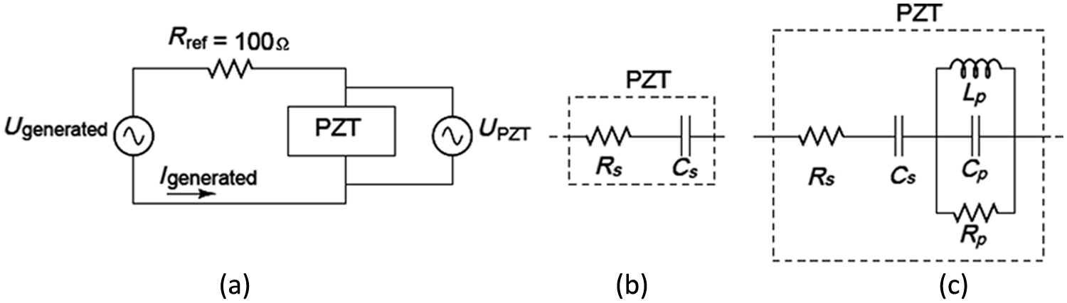
(a) Admittance measurement circuit; (b) resistor–capacitor model for an unloaded PZT below resonance; and (c) more complex inductor–capacitor–resistor model of an unloaded PZT that accounts for resonance and damping.
In a real SHM application, the measured electrical admittance is sensitive to a number of environmental effects such as temperature, pressure, and humidity. 20 In a laboratory environment, temperature changes are most common and must be accounted for. The adjustments to the electrical admittance to compensate for temperature effects can be made using baseline reference admittance measurements over the temperature operating range of the SHM system. In this work, temperature measurements are recorded using an infrared thermometer targeted to the PZT surface prior to taking admittance measurements resulting in consistent admittance data measured at equal baseline temperatures, which can then be compared.
An example obtained experimentally using the admittance measurement circuit of Figure 1(a) is shown in Figure 2 where of the real and imaginary admittance curves are presented for a circular 5-mm diameter PZT transducer unbonded and perfectly bonded to different materials such as glass, aluminum, and carbon fiber composite with properties shown in Table 1 using the same bonding process. These materials are tested as they exhibit different damping ratios that are reflected in the electrical admittance spectrum.
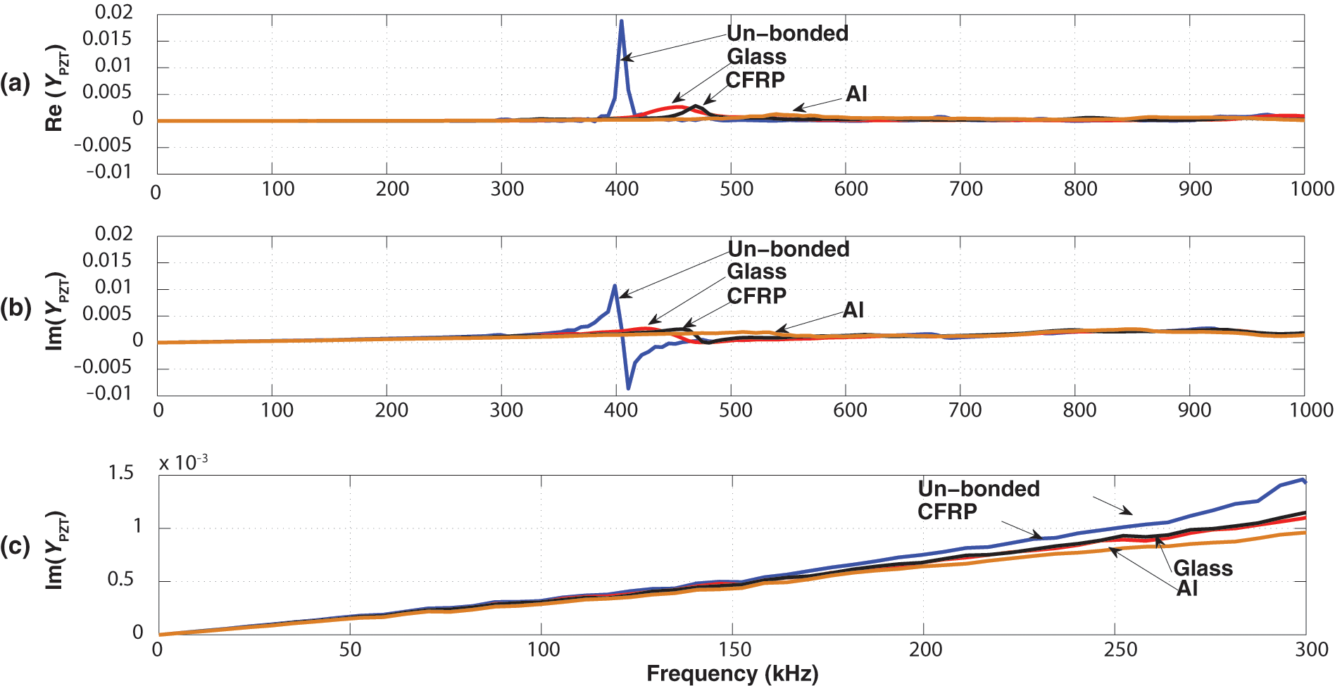
(a) Real and (b) imaginary, and (c) low-frequency zoom of the imaginary electrical admittance curves for a PZT bonded to glass, Al, CFRP, and unbonded.
Material properties for glass, aluminum, and carbon fiber composite.
The electrical admittance spectrum is obtained by sending voltage bursts Ugenerated to the PZT and measuring simultaneously voltage and current using the circuit shown in Figure 1. Prior to this, a reference measurement is performed without the connected PZT that is subtracted from the measured admittance of the PZT to compensate for temperature effects on the measurement circuit. In order to avoid measuring flexural modes from the structure that are classically observed using impedance analyzers based on stationary signal excitation, 9 the broadband generation technique described by Quaegebeur et al. 21 is used over the entire frequency range below 1 MHz. For this purpose, a broadband impulse excitation signal is decomposed over 11 sub-bands. Postprocessing using windowing and reconstruction filters is performed to reconstruct only the electrical contribution of the admittance.
In low frequency (<250 kHz) below the first mechanical resonance, the unbonded and perfectly bonded signals exhibit a linear behavior. As seen in Figure 2(c), there is a significant average decrease in admittance of up to 30% at 250 kHz in the imaginary part between the unbonded and perfectly bonded cases while in the real part there is little change overall for all of the materials. This decrease in the imaginary part of the electrical admittance was also observed by Park et al. 8 and can be associated with a decrease of capacitance measured from the slope of the imaginary admittance curve because bonding the transducer to a host structure directly affects its mechanical compliance. 22 In Figure 2, the amount of change in capacitance between the perfectly bonded and unbonded cases varies depending on the host structure. Aluminum results in the highest capacitive change between the perfectly bonded and unbonded cases. Also, links have been established to variations in the electrical admittance curves through classifying shifts in the curves with respect to an unbonded admittance baseline as increasing in cases of bonding layer degradation, and decreasing with transducer failure. 8 This rule is however only valid below resonance.
As seen in Figure 2, at resonance, the perfectly bonded case results in a decrease in the maximum amplitude of the real part of the admittance and its maximum peak shifts up in frequency compared to the unbonded case. For the imaginary part, a resonance frequency peak is also observed with decreased amplitude and shifts up in frequency with bonding. The resonance effect was reported by Giurgiutiu 5 for low frequency and, to the author’s knowledge, has not yet been exploited as a bonding layer degradation metric.
Observations made in the low-frequency range for both the imaginary and real parts also apply above the first mechanical resonance of the PZT (>700 kHz). The imaginary part of the electrical admittance decreases with bonding and the real part shows a little change. The amount of change in the imaginary part between the unbonded and perfectly bonded state is hard to quantify above the first mechanical resonance of the PZT.
To model the behavioral changes for the electrical admittance Y(ω) in low frequency, a simple RC model can be employed. The model represents the transducer as a simple electrostatic capacitance and a serial resistance as shown in Figure 1(a) and modeled using equation (1) as follows

As frequency increases, due to the finite extent of PZTs, mechanical resonances are observed 5 in the electrical admittance curve such that the simple RC model is no longer valid for modeling PZT electromechanical behavior. In order to derive parameters that take into account PZT resonances, an extended modeling of electrical admittance curves is necessary as shown in Figure 1(b) and modeled using equation (2) as follows
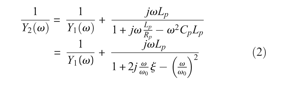
where ω0 is the angular resonance frequency of the PZT and ξ is the modal damping with
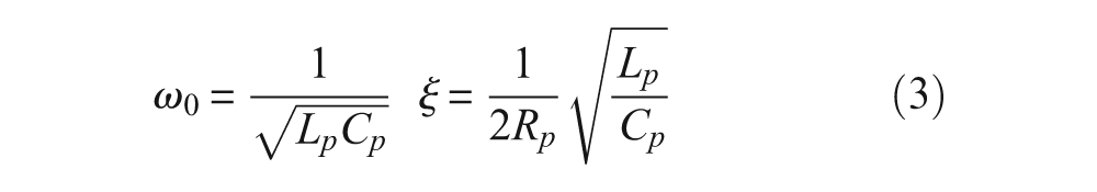
It should be noted that equation (2) is only valid for modeling the first mechanical resonance of PZTs. With increasing frequency, a number of mode shapes and resonances exist within the plate 23 that would require a larger number of band-pass filter LCR circuits. By measuring the bonded PZT electrical admittance, the metrics, resonance frequency ω0, and the modal damping ξ, can be extracted from the imaginary part of the admittance (equation (3)).
In the first step, the electrical parameters in the model given by equations (1) and (2), namely Cs, Cp, Lp, Rp, and Rs, are determined using minimization algorithms (fmincon or ga functions) available within the MATLAB framework. These algorithms are typically used to find the minimum of constrained nonlinear multivariable functions by substituting values over all of the variables starting from an initial estimate for a number of iterations. The initial estimate for each parameter before iterations begin is selected based on the empirical data. The minimization algorithm searches for minimal distance between the modeled and measured admittances, by minimizing the sum of the absolute difference between the modeled and measured admittances for both the real and the imaginary parts. In the second step, the metrics are obtained using equation (3).
The resonance frequency and damping can also be measured manually for quick estimates from the real part of the electrical admittance. At the resonance frequency, the real part forms a large and distinctive peak from equation (2) if
An example of admittance curves obtained with parameter estimation for a bonded transducer case using the genetic minimization algorithm is shown in Figure 3. The minimized parameters are then used with equation (2) to determine the theoretical admittance (dashed line in Figure 3). In general, equations (1) and (2) are analyzed separately to improve parameter estimation results. When using equation (1), the minimization algorithm provides a reasonable estimate of the electrostatic capacitance (Cs) by conforming to the initially linear electrical admittance curve. When using equation (2), the minimization algorithm performs less well in estimating the capacitance with an average underestimate of 5% (shown in Figure 3) but allows for estimating Cp, Lp, and Rp and, with equation (3), the resonance frequency and modal damping metrics are calculated.
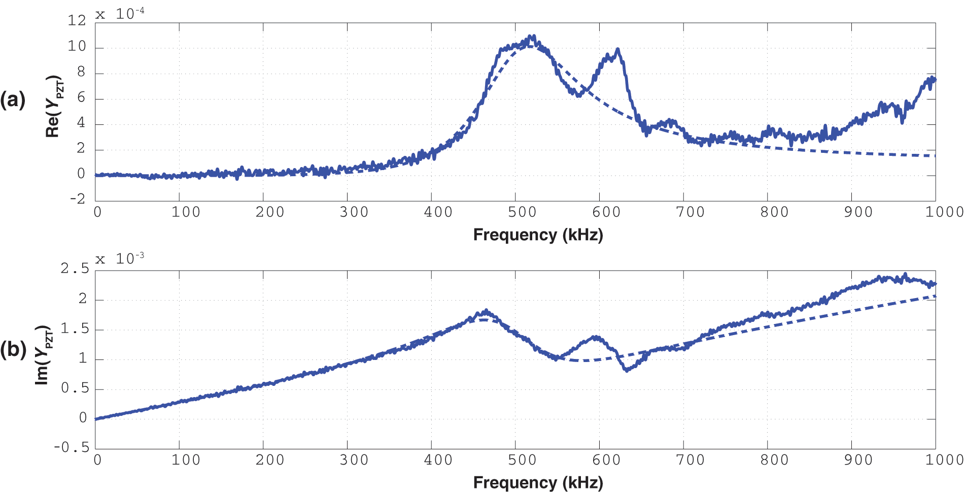
(a) Real and (b) imaginary parts of the electrical admittance for a perfectly bonded PZT (solid) and an approximation (dashed) using equation (2).
The measured real and imaginary parts of the electrical admittance and an approximation using equation (2) are presented in Figure 3 for a perfectly bonded PZT. At PZT resonance, large and sudden changes in the admittance curve are observed. These changes result from the variation of modal damping of the PZT with frequency. In the following sections, numerical and experimental work is presented to determine whether the modal damping is a dominant metric for measuring a gradual debonding of a PZT from a host structure. In contrast, capacitance is only useful for discriminating between perfect bonding and complete debonding.
Numerical and experimental results for quantification of the degradation process
Numerical assessment of the degradation process
The first step in this study is to investigate the degradation process of the bonded PZTs and relate it to the metrics extracted from the electromechanical problem in the ‘Metrics for PZT debonding’ section. For this purpose, a numerical model has first been developed using the commercial FEM software COMSOL. An axisymmetric two-dimensional (2D) model in the frequency domain has been used for simplicity as presented in Figure 4. To mimic the experimental setup used in the ‘Experimental procedure’ section, a 5-mm diameter circular PZT whose characteristics are indicated in Table 2 is attached to a glass sheet using a thick bonding layer of 0.1 mm, whose properties are representative of epoxy (Table 2). The glass sheet is modeled as an isotropic structure with properties defined in Table 2 and perfectly matched layers of 20 mm are used to avoid boundary reflections.
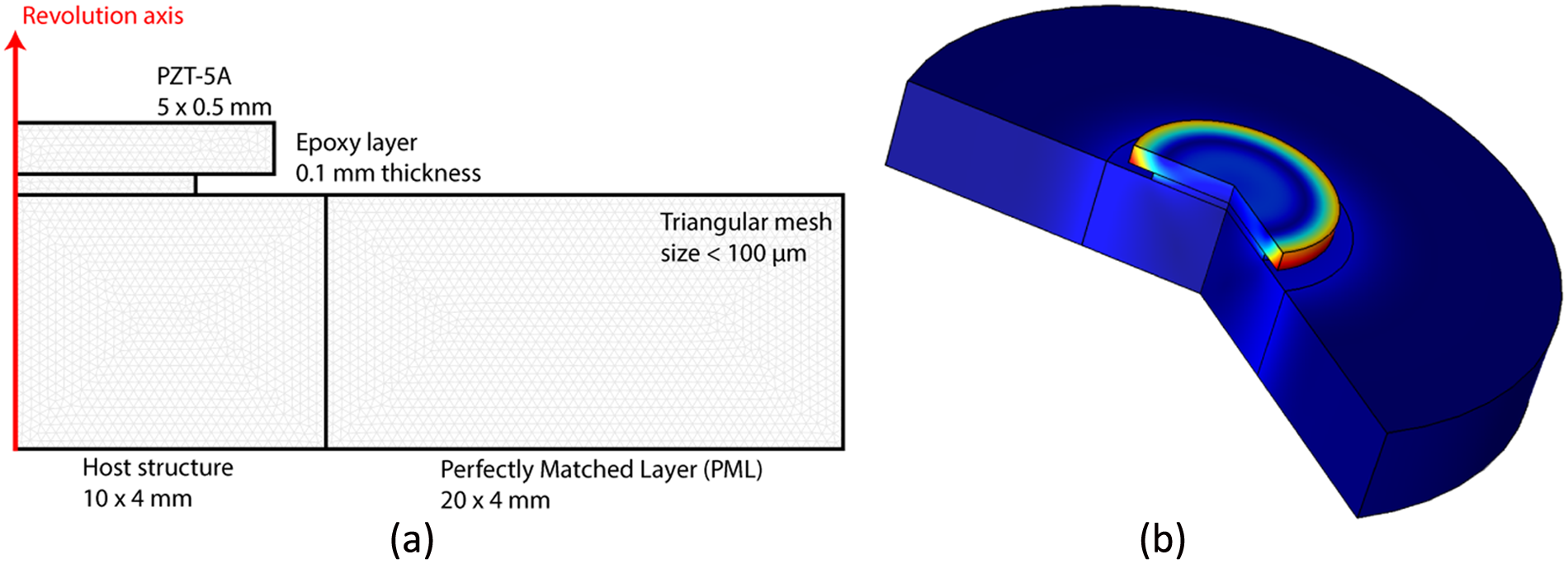
(a) Illustration of the finite element modeling mesh used for computation and (b) three-dimensional reconstruction of the displacement field.
Properties of the PZT transducer and glass sheet.
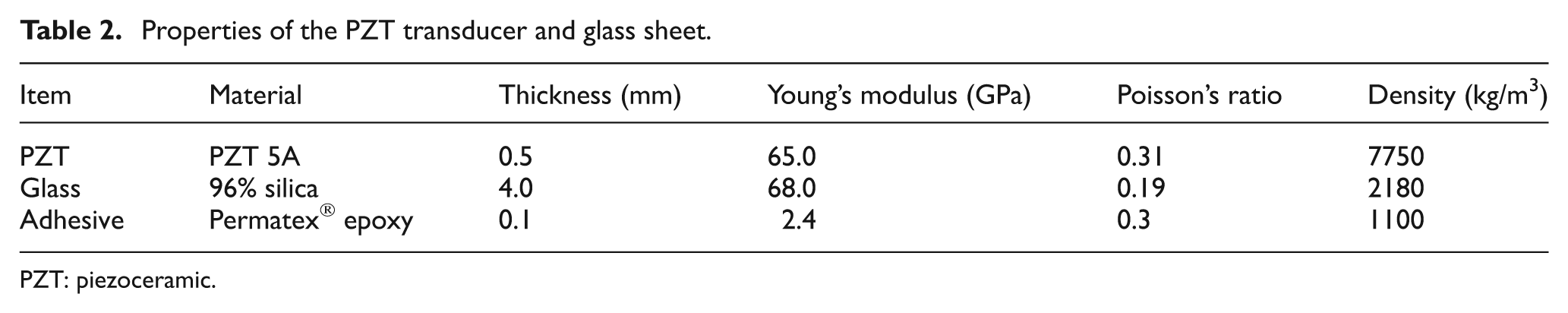
PZT: piezoceramic.
The model is meshed using 15,000 triangular elements for a total number of 60,000 degrees of freedom (DOFs) such that a maximum mesh size of 0.1 mm is ensured and that at least 10 nodes exist per minimum resolvable wavelength. 24 A voltage of 1 V is applied at the upper electrode of the PZT and current is estimated at the same electrode such that electrical admittance can be extracted. The electrostatic capacitance (Cs), angular frequency of the resonance (ω0), and modal damping (ξ) are estimated using methods described in the ‘Metrics for PZT debonding’ section. In this numerical work, two adhesive degradation modes are tested numerically: variation of adhesive coverage and reduction in the Young’s modulus of the adhesive.
For the first degradation mode, the influence of adhesive coverage is estimated by changing the adhesive surface from 100% (perfectly bonded adhesive) to 5% (nearly debonded) by steps of 5%. For the second degradation mode, the adhesive Young’s modulus is varied, and 20 trials are performed by which the adhesive Young’s modulus is decreased by steps of 5% of its nominal value. The results of the simulation are presented in the ‘Numerical and experimental results of bonding layer degradation’ section.
Experimental procedure
Experiments are conducted to relate the degradation process of the bonded PZTs to the metrics extracted from the electromechanical problem through gradual chemical degradation. The adhesive coverage reduction through gradual chemical degradation is chosen in this work because adhesive coverage is easily measurable experimentally compared to changes in the bonding layer Young’s modulus. The changes in the bonding layer modulus are typically quantified by first degrading the adhesive using ultraviolet (UV) light or temperature cycling, and then using traction testing or a rheometer measuring the Young’s modulus. The traction testing and rheometers both require access to the adhesive that is impractical in this study. 25 The effect of chemical bonding layer degradation does however have a slight effect on the adhesive Young’s modulus. 18 The goal of the chemical degradation is to further explore conclusions drawn by Park et al. 8 experimentally under controlled conditions and to extract metrics sensitive to gradual bonding layer degradation.
Transducers are bonded to the surface of a transparent glass sheet with dimensions of 91.5 cm × 50.9 cm and properties described in Table 2 using 0.01 ml of epoxy measured from a syringe and a static load of 125 kPa. In order to weaken the bonding layer, chemical degradation is induced at each trial by injecting 3 ml of acetone via a needle point syringe around and under the area of the transducer over a period of 5 min. Due to the transparency of the glass, a visual assessment of how much adhesive is being removed is performed. Using high-quality photographs, images are analyzed using ImageJ 26 software to quantify the degradation area for each trial. This is performed by manually tracing an estimated initial region of interest (ROI) covering all of the perfectly bonded area and subtracting subsequent ROIs of the degraded areas (Figure 5).
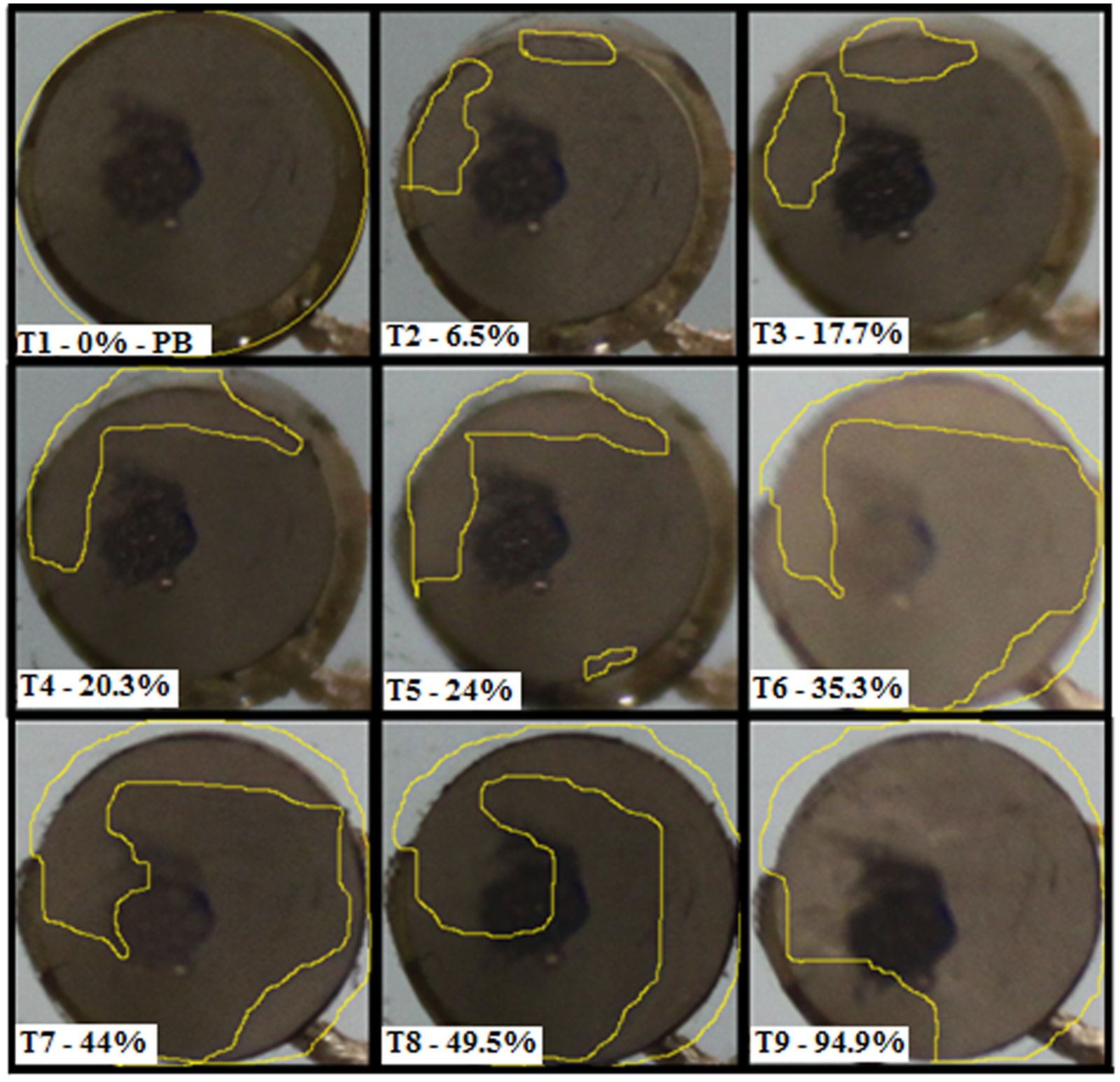
High-resolution photos of the bonding layer for each degradation T taken through the glass host structure. Regions of interest are subtracted from an initial manually traced area estimate to determine the amount of degradation.
As indicated in the ‘Metrics for PZT debonding’ section, voltage bursts are generated at the PZT, and the voltage and current are measured, as shown in Figure 1(a). The input signals are generated using an HP 33120A generator with a sampling frequency of 10 MHz. The generated signals are amplified using a MusiLab UA-8400 amplification system. The signal acquisition is performed using a high-impedance National Instruments® PCI-5105 12-bit DAQ board configured through a custom LabVIEW interface. The signals are recorded at a fixed sampling frequency of 60 MHz. All measurements are averaged 500 times in order to increase the signal-to-noise ratio (SNR) and low-pass filtered at 1.5 MHz. The transfer function for the admittance over the entire frequency range below 1 MHz is obtained using broadband generation of guided waves through sub-band decomposition with N = 10 sub-bands for reconstruction between 10 kHz and 1 MHz as presented by Quaegebeur et al. 21 A sub-band signal frequency step of 100 kHz is selected to ensure perfect reconstruction.
The electrostatic capacitance (Cs) and series resistance (Rs) are estimated based on the slope of the admittance curve from the transfer function in the lower frequency range (<250 kHz) by using the minimization algorithm with equation (1). The inductance (Lp), electrical compliance (Cp), and resistance (Rp) are obtained using the minimization algorithm with equation (2) within the resonance range of the admittance curve (250–700 kHz). The resonance frequency and damping are finally extracted using equation (3). The two frequency ranges are selected based on the PZT resonance. The parameters: Cs and Rs model the shape of the admittance curve below PZT resonance. The starting point of the PZT resonance is observed from the curve in Figure 3 to begin around 250 kHz. To model PZT resonance above 250 kHz, the parameters, Lp, Cp, and Rp, are then used.
Numerical and experimental results of bonding layer degradation
The results for resonance frequency and modal damping along with capacitance (Cs) and the exception of the series resistance (Rs) are individually plotted against the amount of degradation in Figure 6. The series resistance is ignored because of its low value, which is too difficult to measure precisely. The capacitance versus adhesive coverage degradation is presented in Figure 6(a). The simulations show a gradual increase in the capacitance with transducer debonding as presented by Park et al. 8 Experimentally, the unbonded and perfectly bonded points agree well with the simulation results. The intermediate points, however, show large variations between 20% and 40% degradation in the capacitance measurements due to alterations in the mechanical coupling between the transducer and the host structure surface via bonding degradation. This leads to false interpretation suggesting back and forth between bonding layer degradation and transducer damage even though the transducer was not damaged. The capacitance does show an overall tendency to increase over a 20% range with degradation experimentally but is only a valid metric for determining if the transducer is perfectly bonded or unbonded due to resonance that can falsely indicate transducer degradation.
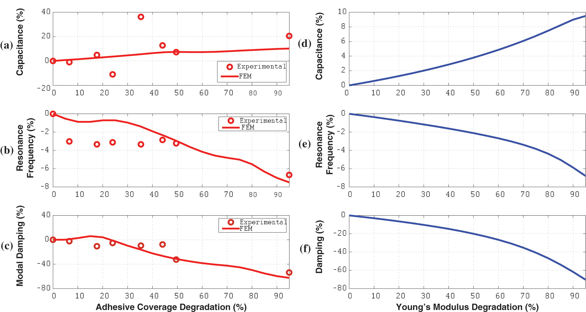
Numerical and experimental results for capacitance, resonance frequency, and damping over adhesive coverage degradation (a–c) and Young’s modulus degradation (d–f).
The numerical results of Figure 6(d) suggest that the capacitance is not only affected by adhesive layer coverage degradation but also by degradation in the adhesive layer Young’s modulus. The degradation in the adhesive Young’s modulus also leads to an increase of capacitance similar to adhesive coverage degradation but over a smaller range. The effect of Young’s modulus on capacitance has never been studied experimentally because the Young’s modulus with each degradation trial is not easily measurable. Taking into account the Young’s modulus effect could improve the closeness of the simulated and experimental results in the capacitance and adhesive coverage area degradation curves.
In Figure 6(b), the resonance frequency is plotted against adhesive coverage degradation. Simulations show a gradual decrease in the resonance frequency with adhesive coverage degradation. This is also seen experimentally, and the perfectly bonded and nearly unbonded points line up very well. Between 5% and 45% adhesive coverage degradation, however, the resonance frequency shows little change and does not retake simulation trends until 50% adhesive coverage degradation. The resonance frequency measurements for PZT transducers with adhesive coverage degradation on a carbon fiber composite coupon by Yu and Gresil 9 showed a range of 100% and a consistent increase in resonance frequency was observed with debonding in low frequency. A 50% jump in the last 45% portion of adhesive coverage degradation was also observed before complete debonding that agrees with the sharp decrease of the resonance frequency metric closer to complete transducer debonding in this study. The resonance frequency metric performs poorly in the range of 5%–45% of adhesive degradation and the severity of the bonding layer cannot be fully evaluated until late in the degradation process (95% degraded).
The numerically simulated resonance frequency versus the adhesive Young’s modulus degradation is presented in Figure 6(e). Simulations show a gradual decrease over a range less than 10% in resonance frequency as the adhesive Young’s modulus is degraded. As previously explained, the degradation of the Young’s modulus is not easily determined experimentally. The points that do not line up between 5% and 45% degradation in Figure 6(b), however, may further support that adhesive degradation is not only a matter of coverage area but also a change in the Young’s modulus as described by Skaja et al. 18
The modal damping metric is presented Figure 6(c). Simulations show that damping gradually decreases with adhesive coverage over a range of 80%. Experimentally, the same tendencies as in the simulation curve are observed with fairly good agreement. The modal damping metric such as the resonance frequency metric is robust but has the advantage of an increased range with up to 80% in variation between the perfectly bonded and debonded states. Although the experimental points are in good agreement with simulated results, some points differ up to 20% from the simulated curves. This again suggests a need to incorporate the Young’s modulus effect presented in Figure 6(f) from simulation that shows the same decrease in modal damping with adhesive Young’s modulus degradation. Although simulation results show that bonding layer degradation is a combination of adhesive coverage and Young’s modulus degradation, experimental results could only be compared to the adhesive coverage failure mode as the Young’s modulus decay with each degradation step was not measured. Even though the modal damping metric shows the largest range between the perfectly bonded and nearly debonded cases, the range of the capacitance, resonance frequency, and modal damping metrics is material-dependent as shown in Figure 2.
Effects of degradation on actuation and sensing of guided waves
Experimental setup
In order to relate the bonding degradation to the actuation and sensing performance of guided waves using a PZT, the influence of adhesive layer degradation in a PC configuration is proposed in this section.
The experimental setup is presented in Figure 7. The transducers are separated by a distance of 20 cm, and fixed to a sheet of glass (91.5 cm × 50.9 cm) using epoxy with properties presented in Table 2. One transducer is used as a reference, while the other one is used for evaluation of both a degraded actuator and sensor. The PC configuration is surrounded by an absorbing perimeter to attenuate edge reflections. The transducers are placed 20 cm apart from the edges of the glass sheet. Chemical adhesive coverage degradation is again used.
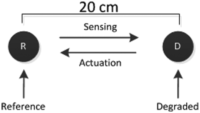
Experimental setup for the pitch-catch configuration with a reference PZT (R) and degraded PZT (D).
The broadband generation of guided waves through sub-band decomposition technique presented by Quaegebeur et al. 21 is used to estimate the transfer functions for amplitude and phase versus frequency below 1 MHz. For a given adhesive coverage degradation, the reference transducer first generates the broadband signals and the degraded transducer is used as a sensor response to estimate the effect of degradation on sensing. Then the degraded transducer is used as an actuator and the reference transducer as a sensor. To determine the effect of degradation on actuation, the amplitude and phase are then frequency averaged for both actuation and sensing for three frequency ranges: low frequency (<250 kHz), around mechanical resonance (250–700 kHz), and above resonance frequency (>700 kHz). The adhesive coverage degradation is obtained visually as in the ‘Experimental procedure’ section. The error bars are calculated from the standard deviation of each frequency range. The sample size for each standard deviation is approximately 1365 frequency points, which is a third of the 4096 frequency points used for each signal fast Fourier transform (FFT). The amplitude and phase are presented in Figure 8 for sensing and in Figure 9 for actuation.
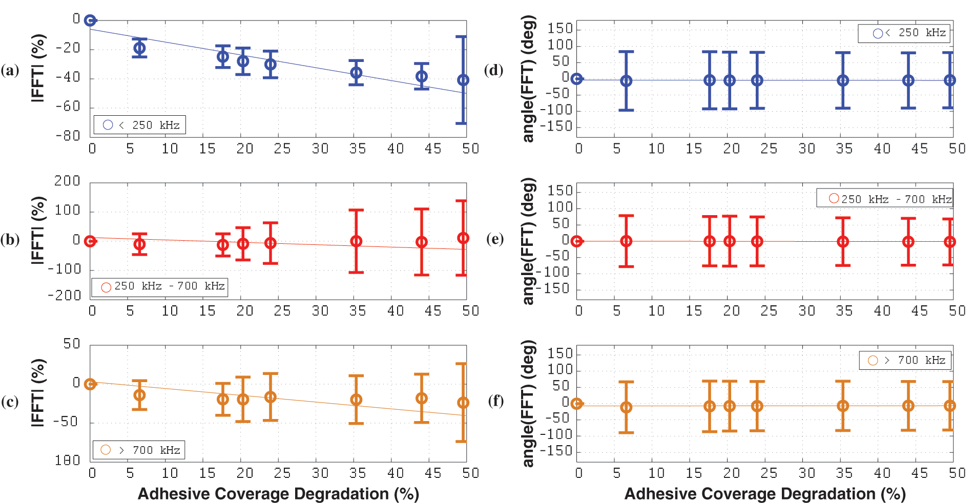
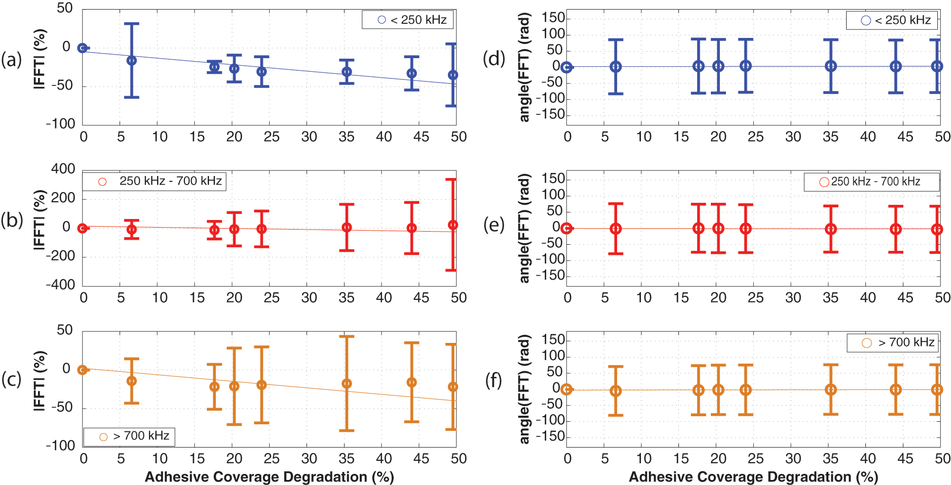
Changes in the (a–c) amplitude and (d–f) phase of sensor signals with adhesive coverage degradation for three frequency ranges (<250 kHz: (a), (d); 250–700 kHz: (b), (e); >700 kHz: (c), (f)).
Changes in the (a–c) amplitude and (d–f) phase of actuation signals with adhesive coverage degradation for three frequency ranges (<250 kHz: (a), (d); 250–700 kHz: (b), (e); >700 kHz: (c), (f)).
Impact of sensor degradation
The amplitude change for a PZT used as a sensor versus adhesive coverage degradation below resonance is presented in Figure 8(a). With degradation, a linear decrease in amplitude is observed. There is an overall decrease of 50% in signal amplitude between the perfectly bonded and 50% unbonded stages in adhesive area degradation. 9 This suggests that degradation of the bonding layer coverage area has an effect on the relative transmitted energy from the host structure to the PZT. Another observation that can be made in Figure 8(a) is that the error bars increase with degradation of the adhesive coverage. These increases are associated with local spectrum changes toward low frequency with degradation as observed by Yu and Gresil. 9 The average amplitude over the low-frequency range is being measured and, therefore, resonance peaks have significant effects on averaging resulting in large standard deviations. The overall tendency of the amplitude below resonance up to 45% adhesive coverage degradation is decreasing and insensitive to resonance.
The amplitude change versus adhesive coverage degradation around resonance is presented in Figure 8(b). The main difference from below resonance is that error bars become larger earlier on in the degradation at 20%. This signifies a large variability in the frequency spectra as observed in this frequency range.
The amplitude change versus adhesive coverage degradation above resonance is presented in Figure 8(c). The results exhibit the same behavior as below resonance in Figure 8(a), with an overall decrease in amplitude with degradation but larger error bars are observed above 20% degradation as in the resonance range. The decrease in amplitude is a combination of a reduction in the relative transmitted energy between the host structure and the PZT but also because degradation causes resonances to shift out of the high-frequency range as observed in Figure 2. The existence of resonance yields larger error bars but the error bars are on average 50% smaller than in the resonance range because the resonance peaks are shifting out of the high-frequency range.
The phase change versus adhesive coverage degradation below, around, and above resonance is presented in Figure 8(d)–(f). In Figure 8(d), the phase of the sensor signal below resonance is presented. With degradation, the phase decreases slightly (1°) from the perfectly bonded case. In Figure 9(e), the phase of the sensor signal around resonance is presented. Again, the results show a linear decrease with degradation slightly deviating from the perfectly bonded case. For frequencies above resonance shown in Figure 9(f), the phase shift is more significant. After an initial degradation of 10%, the phase decreases by 11° from the perfectly bonded case. With further degradation, the phase increases linearly up to 5° for an adhesive coverage degradation of 50%.
Overall, the three frequency ranges are affected differently. The effect of the bonding layer is related to its density, thickness, and surface coverage area, 27 and changes to these parameters through degradation affect the interaction between the transducer and the host structure. The changes to the bonding layer stiffness have been investigated by Pietrzakowski 28 and these changes tend to decrease the PZT signal amplitude. In this case, the amplitude in all three selected frequency regimes shows a similar overall change. However, the phase above resonance shows the largest change over the other frequency regimes with degradation. In the case of the amplitude, the resonance frequency signals show the largest error bars, suggesting that the amplitude in the resonance frequency range is influenced the most with changes to the bonding layer properties.
Impact of actuator degradation
The amplitude change versus adhesive coverage degradation for a PZT used as an actuator is presented in Figure 9. In each case, for amplitude (Figure 9(a)–(c)), the actuator mimics the same tendencies as the sensor with degradation over the same ranges. The resonance frequency regime of the amplitude shows the largest influence with respect to error bars compared to the other regimes.
The phase change versus adhesive coverage area degradation is presented in Figure 9(d)–(f). In Figure 9(d), the phase of the actuator signal below resonance is presented. Over the entire adhesive degradation range, there is a linear increase in phase of 1° from the perfectly bonded case. In Figure 9(e), the phase of the actuator signal around resonance is presented. Opposite to low frequency, the phase decreases linearly up to 2° from the perfectly bonded case. In frequencies above resonance shown in Figure 9, a linear increase in phase of 3.5° over the degradation range is observed. Similar tendencies are observed for the actuation phase when compared to the sensor phase curves. In both cases, high-frequency signals demonstrate the highest phase change with degradation. It has also been found in literature that bonding layer degradation effects generated signal phase in low frequency by Overly et al. 20 that could lead to false indications on structural conditions but the effect has not been studied in regimes higher than resonance.
SCF for PC measurements
Using the information, the amount of adhesive coverage degradation obtained through the modal damping metric and curves that describe changes in amplitude and phase from the perfectly bonded state, an SCF is proposed and assessed in the following. The SCF removes biasing in SHM-gathered signals caused by bonding degradation to potentially improve structural damage estimates. 22
The signal measured by a transducer within an SHM system could show variation by degradation of the host structure

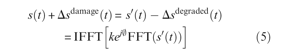
With knowledge of the change in amplitude and phase for a given degradation and the frequency range of the generated signal, the captured signal can be adjusted to compensate for bonding layer degradation. A formulation for removing the PZT degradation effect thus revealing signal changes due only to structural damage is shown in equation (6) where the amplitude of the measured signal
For the SCF, a linear curve fit is used to approximate the changes in amplitude and phase with adhesive coverage degradation to the curves in Figures 8 and 9. The amount of adhesive coverage degradation can be estimated from the modal damping metric; calculated following the electromechanical characterization described in the ‘Experimental procedure’ section, and then using the FEM curves in Figure 6(c). To test the correction factor, signals are generated and measured below, around, and above resonance. The signals falling in each of the selected frequency ranges: 150, 400, and 700 kHz along with adjusted signals using the SCF are first presented for a degraded sensor in Figure 10. In the following, it is assumed that the damping metric was evaluated for a given PZT and that this leads to an evaluation of the degradation of 15%. The perfectly bonded and 15% degraded signals are then derived from the measured transfer functions created using sub-band decomposition described in the ‘Numerical and experimental results for quantification of the degradation process’ section. The amplitude and the phase changes are obtained from the curves in Figure 8 for the respective frequency range and the degraded signal is adjusted.
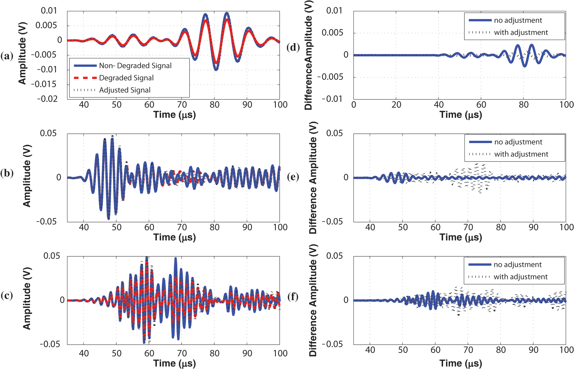
Degraded, nondegraded, and adjusted signals (a) below, (b) at, and (c) above resonance with differences between signals with and without adjustment (d) below, (e) at, and (f) above resonance for the sensor.
The degraded, nondegraded, and adjusted signals below resonance are presented in Figure 10(a). The degraded signal after 15% adhesive coverage area degradation shows a 25% decrease in the peak amplitudes of both the A0 and S0 modes (Figure 8(a)). A slight phase shift also exists (Figure 8(d)). The difference between the perfectly bonded and nonadjusted signal with the difference between the perfectly bonded and adjusted signals is plotted in Figure 10(d). The amplitude variation has been reduced by 96% and the phase difference has also been reduced after using the SCF.
The degraded, nondegraded, and adjusted signals at resonance are presented in Figure 10(b). The degraded signal after 15% adhesive coverage area degradation shows a 10% decrease in both the peak amplitude of the A0 and S0 modes (Figure 8(b)). Again, a slight phase shift exists (Figure 8(e)). The difference between the perfectly bonded and nonadjusted signal with the difference between the perfectly bonded and adjusted signals is plotted in Figure 10(e). The amplitude variation has been reduced by 50% and the phase difference has also been reduced. At resonance, edge reflections begin to interfere with the traveling A0 and S0 modes (around 65 µs) and, therefore, phase correction does not appear to have a large effect but does however on the maximum amplitudes, which is a key for imaging algorithms.13,14
The degraded, nondegraded, and adjusted signals above resonance are presented in Figure 10(c). The degraded signal after 15% adhesive coverage degradation shows a 10% decrease in both the peak amplitude of the A0 and S0 modes (Figure 8(c)). As in the previous frequency ranges, there is a slight phase shift (Figure 8(f)). The difference between the perfectly bonded and nonadjusted signal with the difference between the perfectly bonded and adjusted signals is plotted in Figure 10(f). The amplitude variation has been reduced by 10% and the phase difference has also been reduced. Above resonance, an increased number of edge reflections plague the traveling A0 and S0 modes and, therefore, phase correction has little effect on signal correction. The maximum amplitudes are still preserved for the two modes. It is important to notice that the SCF performs poorly as frequency increases. This is likely due to edge reflections that could be reduced by moving the transducers further from the edges of the plate or adding a thicker absorbing border to the plate.
A similar study was conducted for the actuator. The signals generated and measured in each of the selected frequency ranges: 150, 400, and 700 kHz with degraded actuator along with adjusted signals using the SCF are presented in Figure 11 for 15% degradation. The signal degraded in the same way as those of the sensor. The degraded, nondegraded, and adjusted signals below, at, and above resonance are presented in Figure 11(a)–(c) respectively. The difference between the perfectly bonded and nonadjusted signal with the difference between the perfectly bonded and adjusted signals below, at, and above resonance are shown in Figure 11(d)–(f) respectively. As in the sensor cases, the amplitude adjustment performs poorly as frequency increases and phase adjustment becomes less significant. Edge reflections have a large effect on the signal and cause difficulties in signal correction. But for frequencies below 400 kHz, the SCF for both the sensor and actuator makes a significant difference. It is in this frequency range that most imaging algorithms using PZT transducers operate.13,14
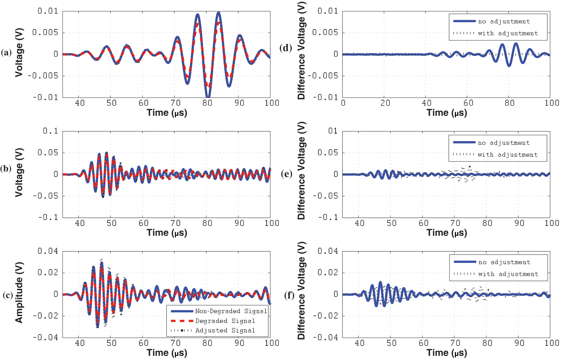
Degraded, nondegraded, and adjusted signals (a) below, (b) at, and (c) above resonance with differences between signals with and without adjustment (d) below, (e) at, and (f) above resonance for the actuator.
In order to better assess the SCF for an extended frequency domain, the effect of the SCF applied to the A0 and S0 modes is presented in Figure 12 first for a degraded sensor for 15% degradation. The amplitude of each mode is extracted separately from the dispersion curves constructed from the signals using sub-band reconstruction 21 used in the ‘Numerical and experimental results for quantification of the degradation process’ section over the frequency range below 1 MHz. The SCF performs well in adjusting the amplitude of the A0 mode below up to 400 kHz. At resonance, the SCF is unable to adjust the amplitude enough to match the nondegraded signal with a 40% difference. For the S0 mode, the SCF performs very well in adjusting for amplitude and frequency shifts below, at, and above resonance. Amplitude compensation works over the entire frequency range below 1 MHz. A slight variation less than 5% can be observed between 500 and 700 KHz between the adjusted and nondegraded amplitudes. Good performance of the SCF in low frequency below resonance for the A0 and S0 modes is critical in imaging algorithms such as EUSR 13 and excitelet 14 as they strongly depend on estimating the time-of-flight (ToF) and amplitude of these wave packets in the low-frequency regime.
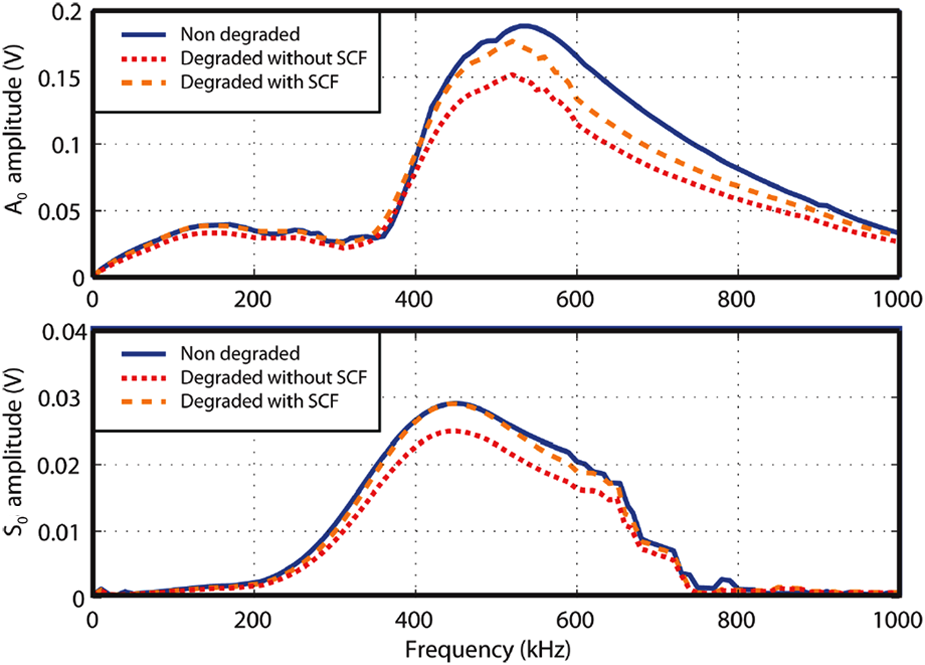
Degraded, nondegraded, and adjusted A0 and S0 modes using the SCF for the sensor.
The effect of the SCF applied to the A0 and S0 modes is then presented in Figure 13 for a degraded actuator. The result of using the SCF on the actuator A0 and S0 modes is comparable to the sensor case. The SCF performs well in adjusting for amplitude and frequency shifts below, at, and above resonance. This indicates that degraded actuators are still able to inject high-quality signals into host structures. Again, at resonance, however, the fit between the nondegraded and corrected signal is not as good as below and above resonance. This is due to the large ranges that were defined for applying the SCF. As previously described in the ‘Experimental setup’ section, the average magnitude and phase over the entire resonance frequency range are used to develop the SCF. This result can be improved by defining narrower ranges for resonance.
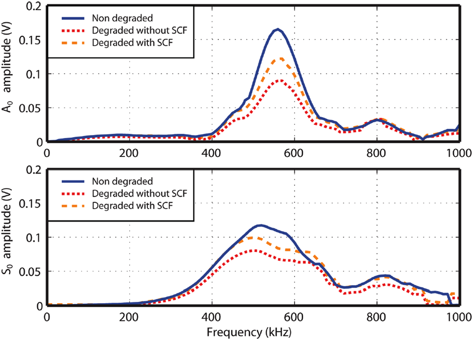
Degraded, nondegraded, and adjusted A0 and S0 modes using the SCF for the actuator.
Conclusion and discussion
In this article, numerical and experimental investigations of metrics to assess and compensate the degradation of the adhesive layer of surface-bonded PZT transducers for SHM applications are presented. Capacitance that is classically derived from the low-frequency electrical admittance appears inadequate for assessing the health of the bonding layer at the first mechanical resonance of the PZT. Modal damping shows a more gradual change when nearing complete bonding layer failure. Modal damping curves suggest that the amount of bonding layer degradation is measurable. Adhesive coverage degradation and Young’s modulus degradation tend to have the same effect on the metrics. Adhesive degradation leads to a reduction in the actuation and sensing amplitude and at higher frequencies, a delay in the time signal is observed. With this information, an SCF is used to adjust signals generated or sensed from PZT transducers with a degraded bonding layer. The SCF is able to better adjust the A0 mode than the S0 mode at low-frequency regimes in sensing and performs well in adjusting both modes for actuation over the entire frequency regime up to 1 MHz. A practical example was demonstrated for the A0 and S0 amplitudes that can be useful in existing imaging algorithms. Therefore, this article has shown that an SCF based on the level of degradation from electrical modal damping measurements can be used to compensate for amplitude and phase changes. As presented in this article, the SCF relies heavily on empirical data for developing damping, amplitude, and phase curves with degradation. In future work, the numerical model will be employed to derive such curves and thus reduce experimental uncertainties.
Footnotes
Acknowledgements
The authors would also like to acknowledge Etienne Yvain, Victor Canel, and Adrien Brunel for their contributions to this project.
Funding
This study has been conducted with the financial support from the Natural Sciences and Engineering Research Council of Canada (NSERC) and the National Research Council of Canada (NRC).