
Abstract
The use of condition monitoring data for diagnostic and prognostic of vehicle health has been growing with increasing use of health and usage monitoring systems. In this article, an approach using the switching Kalman filter framework is explored for both diagnostic and prognostic using condition monitoring data under a single framework. The switching Kalman filter uses multiple dynamical models each describing a different degradation process. The most probable underlying degradation process is then inferred from the observed condition monitoring data using Bayesian estimation. By using the dynamical behavior of the degradation process, pre-established fault detection threshold is no longer required. This approach also provides maintainers with more information for decision-making as a probabilistic measure of the degradation processes is available. This helps maintainers to predict remaining useful life more accurately by distinguishing between the degradation states and performing prediction only when unstable degradation is detected. The proposed switching Kalman filter approach is applied onto sets of condition monitoring data from gearbox bearings that were found defective from the Republic of Singapore Air Force AH64D helicopter. The use of in-service data in a practical scenario shows that the switching Kalman filter approach is a promising tool for maintenance decision-making.
Keywords
Introduction
With the increasing use of health and usage monitoring systems on vehicles in the past decade, traditional corrective and preventive maintenance is rapidly evolving toward condition-based maintenance (CBM). The use of condition monitoring (CM) data for fault diagnosis and prognosis of remaining useful life (RUL) is a key element in a CBM program and much research was undertaken on their approach and methodologies. A comprehensive survey of these methods was conducted by Heng et al., 1 Jardine et al., 2 and Sikorska et al. 3 and their works showed that the methods can be grouped into three main categories, namely, machine learning, statistical, and model-based methods. Both machine learning and statistical methods such as neural networks 4 and hidden Markov models (HMMs) 5 can model highly nonlinear problems and different failure modes, respectively, but they require a large number of datasets to train the models that are often not available in practice. As such, most of the published works are performed using experimental or simulated data and actual fielded applications are rare. Model-based method uses mathematical representation of the system’s physical or degradation behavior such as the Paris law for crack propagation. 6 Such methods require less training data, but knowledge of the system’s degradation process is required. The Kalman filter (KF) is a model-based method that has been researched for diagnostics and prognostics.7–10 However, it has limitation in automated and online applications as CM data have to be manually censored for the appropriate degradation model to be used. In this article, the switching Kalman filter (SKF) is proposed to track the degradation processes as it evolves. It is applied on in-service CM data from defective gearbox bearings gathered from AH64D helicopters belonging to the Republic of Singapore Air Force (RSAF). The article is organized as follows: section “The KF and its limitations” discusses the KF and its limitations and section “Background on the SKF” provides the background of SKF. Section “AH64D tail gearbox bearing and CM data” describes the failure findings of the gearbox bearings and section “SKF model description for bearing degradation” shows the SKF formulation for bearing degradation. Sections “Diagnostic of bearing degradation” and “Prognostic of bearing RUL” discuss the SKF diagnostic and prognostic results and compare it to the use of the KF alone.
The KF and its limitations
The KF is a stochastic filtering process that recursively estimates the state of a dynamic system in the presence of measurement noise and process noise by minimizing the mean squared error. 3 The KF consists of a discrete state-space model describing the evolution of a process given by


where xt is the true but hidden state of the system and yk is the observable measurement of the state. The KF assumes a linear system dynamics and all noise follows a Gaussian distribution. A is the fundamental matrix describing the system dynamics and H is the measurement matrix.
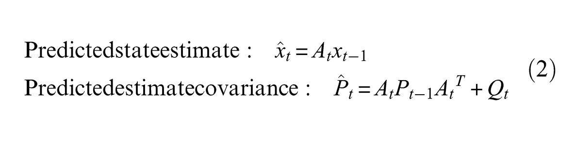
Prediction step:
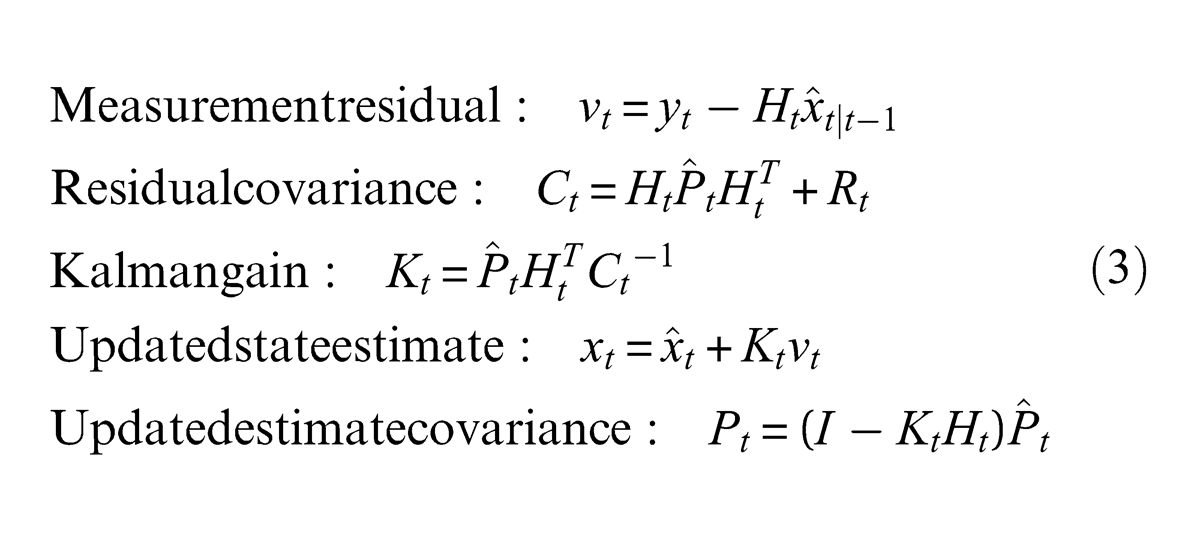
Update step:
The KF has been used in a wide range of applications from navigation and tracking to economic forecasting. In maintenance application, it has been applied to engine health diagnostics 12 and in recent years to electronics prognostics for estimating RUL of ball grid array connections7–9 and electrolytic capacitors. 8 The key advantage of using KF for diagnostics is that it accounts for measurement and system noise in the CM data and the system state and parameters of the degradation model can be adaptively estimated as they evolve through time. 13 It can also be used for prognostics by forecasting the system state into the future using the degradation model and the latest available measurement. For nonlinear system dynamics or non-Gaussian noise, particle filtering can be applied instead of the KF. 14 The use of particle filtering, however, can be very computationally intensive as Monte Carlo simulation is employed heavily in the procedure to estimate the non-Gaussian distributions.
A limitation of the KF is that the system’s degradation process has to be time-invariant, else the model can be unstable and its estimations divergent. In practice, the degradation process in components can change over time. For example, in Figure 1, the vibration measurement of a serviceable bearing can be stationary with measurement noise. When slow stable wear from damage such as surface pitting occurs, the vibration level gradually rises linearly. When the accumulated damage is severe, the vibration level then rises exponentially. The use of a single degradation model would result in inaccurate state estimates and cause RUL predictions to diverge or fluctuate depending on whether the underlying degradation process is under- or over-fitted by the model. In lieu of this, model-based prognostic works often only use portion of the CM data that fit the assumed degradation model9,15,16 and this data censoring has to be performed manually. Furthermore, it is difficult to determine when the assumed model can be suitably applied in an online application where the complete CM history prior to failure is unknown. Thresholds that distinguish the different degradation processes may be established,15,16 but this would require several failure histories which again are hard to obtain in practice. As such, the use of KF for automated and online applications can be challenging. In this article, the use of SKF is proposed to address these challenges.
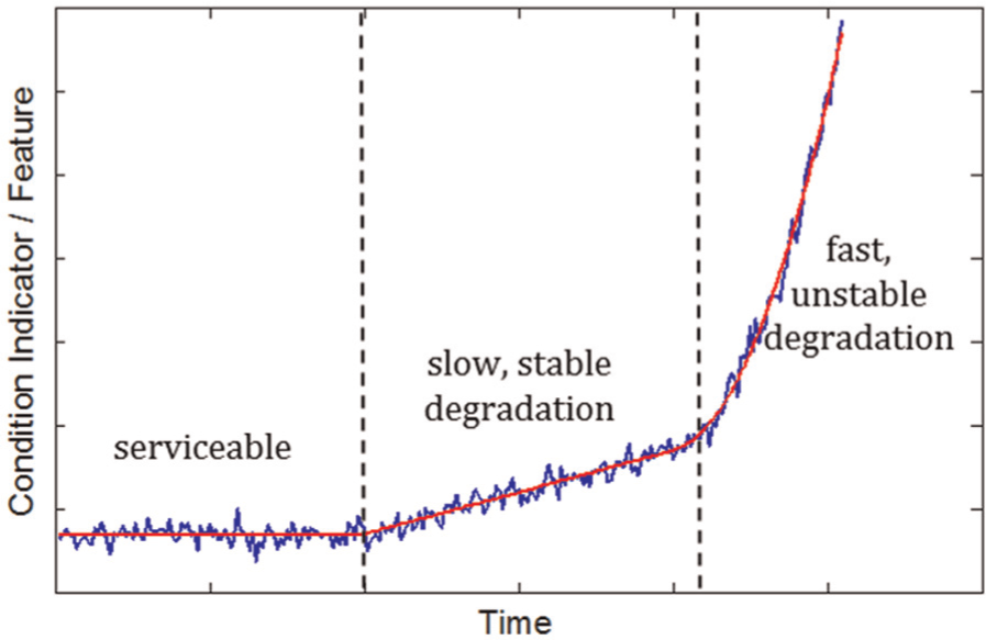
Evolution of degradation process across time.
Background on the SKF
The SKF, also known as linear dynamic models, 17 is used when the dynamical behavior of a process changes and cannot be modeled by a single model. It is popularly used to track multiple moving targets 18 but has been applied in meteorology 19 and econometric 20 as well. In maintenance, it has been used to detect sensors and actuator failures, 21 changes in nonlinear stochastic systems, 22 and in bearing fault prognosis simulation to combine results from different prediction models. 10 The SKF model can be represented as a dynamic Bayesian network as shown in Figure 2. In each time step, both the model switch variable, St, and state variable, xt, are hidden and have to be inferred from the observations, yt. For a system with multiple dynamics that are described with n KFs, the size of the belief state will increase exponentially at each time step to nt. As such, inferring the probability of every state at each time step becomes intractable.
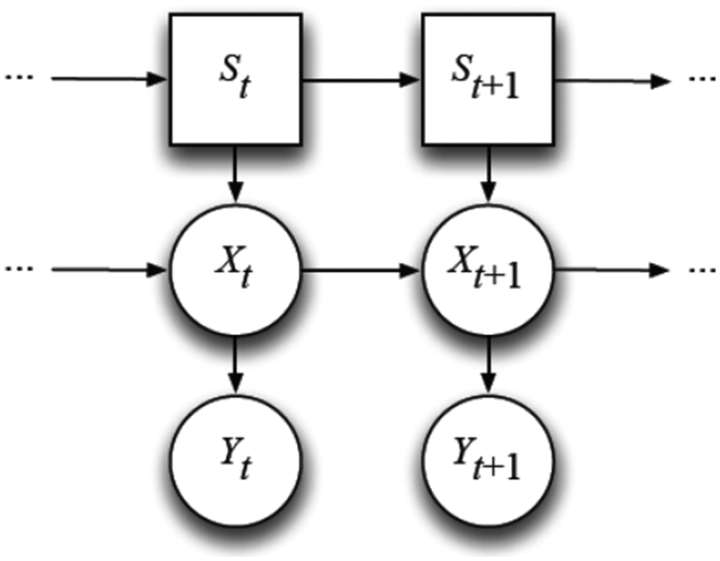
Dynamic Bayesian network representation of a SKF. 17
To overcome this problem, approximation methods like the generalized pseudo-Bayesian (GPB) algorithm as described in Kevin
17
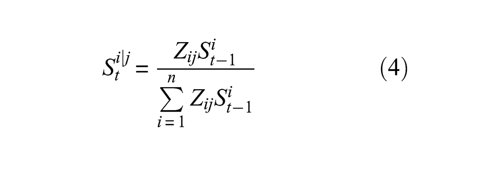
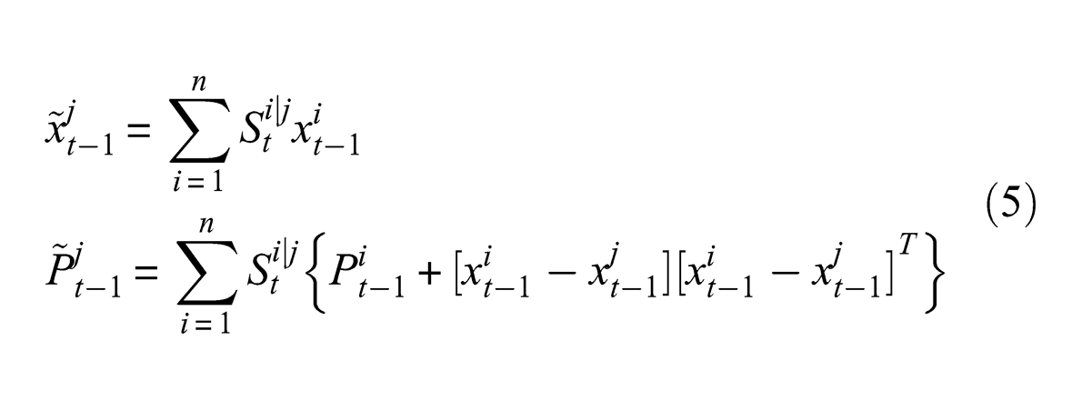
are adopted. In each time step, the state and covariance estimates from all the filters in the previous time step are combined or “collapsed” together with weights assigned according to the model switch variable,
Model switching probabilities
Weighted state and covariance estimates
Likelihood of filter from measurement residual
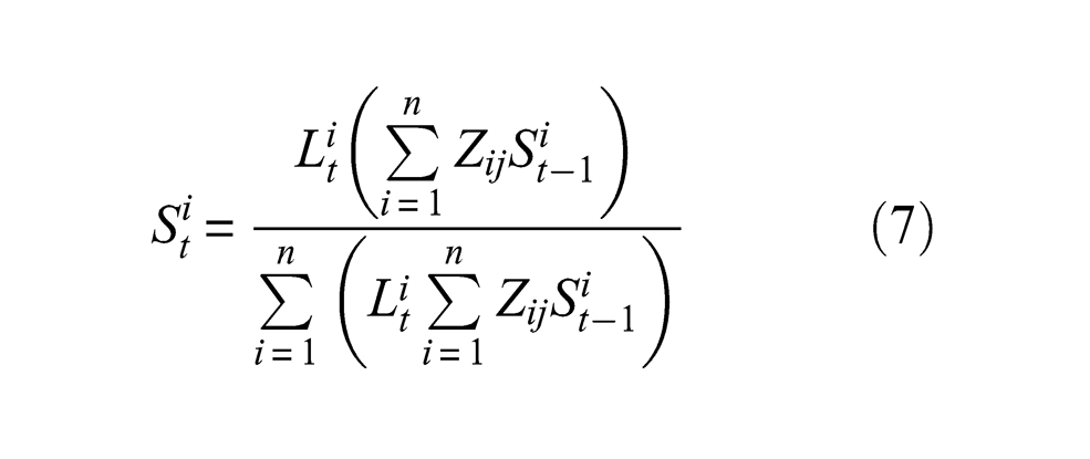
Probability of each model
With the weighted state and covariance estimates, the usual KF as shown in equations (2) and (3) is carried out for each filter model with each yielding a predicted state,
AH64D tail gearbox bearing and CM data
The SKF method shown is applied on the tail rotor gearbox (TRGB) output shaft thrust bearing CM data of the AH64D helicopter from the RSAF. The TRGB is a grease lubricated single-stage gearbox and serves to transmit drive torque from the intermediate gearbox to the tail rotor system. From maintenance records, three TRGBs were found with widespread pitting on ball elements and spalling in the bearing races as shown in Figure 3. The CM data for the TRGBs, which consists of fast Fourier-transformed acceleration spectrum from over 900 flights, were downloaded for analysis. The onboard systems measure vibration levels whenever the aircraft is on ground with rotors at flat pitch and rotating at 101% r/min. This provides a controlled flight condition in which the vibration measurements are taken. From the acceleration spectrum of the four TRGBs, vibration energy can be observed to rise at the bearing ball pass frequency inner (BPFI) race 25 as shown in Figure 4. The CM measure adopted is the root-mean-square (RMS) acceleration, Grms, of the frequency magnitudes in the low-frequency band of 250–2500 Hz to capture the peaks of the BPFI harmonics. A rejection band of 0–250 and 1250–1600 Hz is applied to eliminate effects from the tail shaft frequency, the dominant gear mesh frequencies, and sidebands. A general trend of stationary, linear, and then exponential rise can be seen across the TRGBs, but the rate and duration in each stage differ between individual gearboxes as shown in Figure 5.
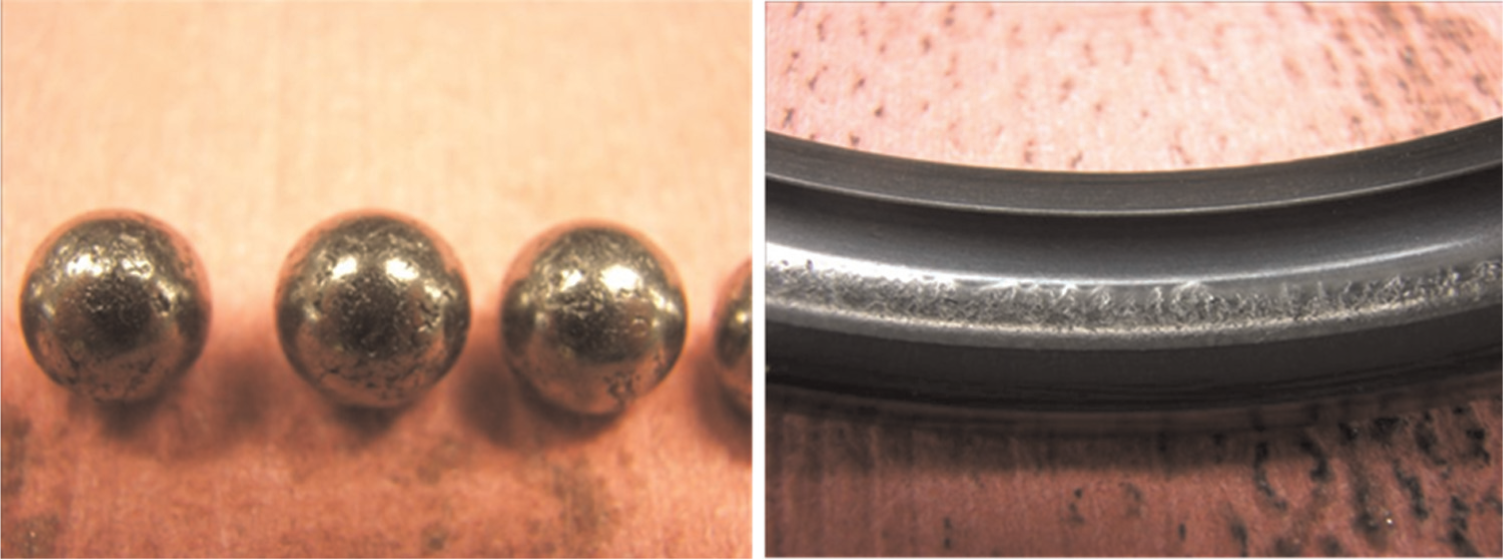
Severe pitting of rolling elements and spalling of bearing races.
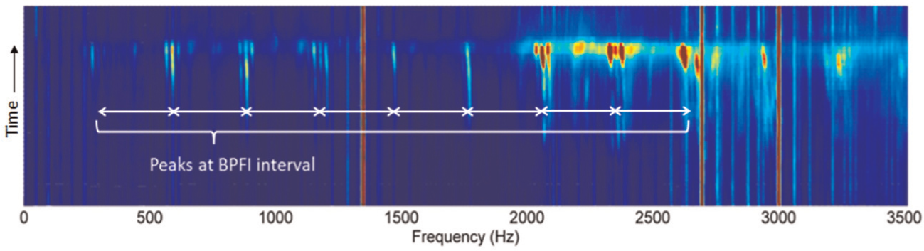
TRGB time–frequency plot showing rise in vibration energy.
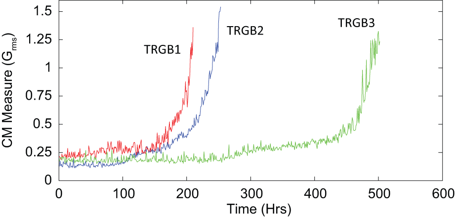
Extracted CM measurement plot for three defective TRGBs.
As the actual time at which the bearing degradation processes transits cannot be physically observed, they are inferred using piecewise or segmented regression 26 on the complete CM data history of TRGB 2 as shown in Figure 6. The CM history is segmented into the three degradation stages with two transition times or “breakpoints.” Zero-, first-, and second-order polynomial regressions are then applied to the segmented CM data for each degradation stage and the sum of their residuals is obtained. This procedure is repeated iteratively with different sets of transition times and the optimal piecewise regression fit is obtained from the set of transition time that minimizes the sum of the residual. Figure 6 shows the transition times for the degradation stages are at 87 and 202 h for TRGB 2. Although these may not be the real transition time, the piecewise regression provides the optimal fit for each stage of the degradation process. In practice, the complete CM history will not be available, and thus, the SKF is used as a decision support tool to diagnose the different stages of bearing degradation. When the degradation is diagnosed to be fast and unstable, the RUL of the gearbox bearing is then estimated. RUL estimation is not carried out during the stable wear as the prediction will be overestimated although maintainers may choose to monitor the condition more frequently. It is possible to establish a threshold limit for the onset of unstable wear if adequate past failure datasets are available to predict the time before unstable wear occurs. It is not considered here, however, as the goal is to estimate the RUL.
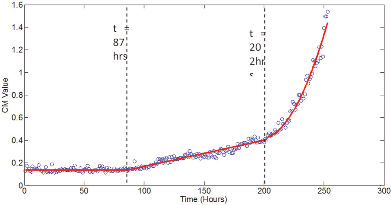
Degradation stages for TRGB 2 inferred from piecewise regression.
SKF model description for bearing degradation
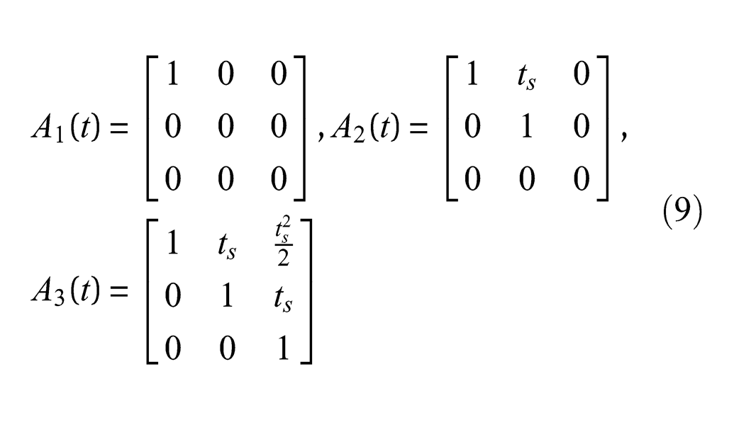
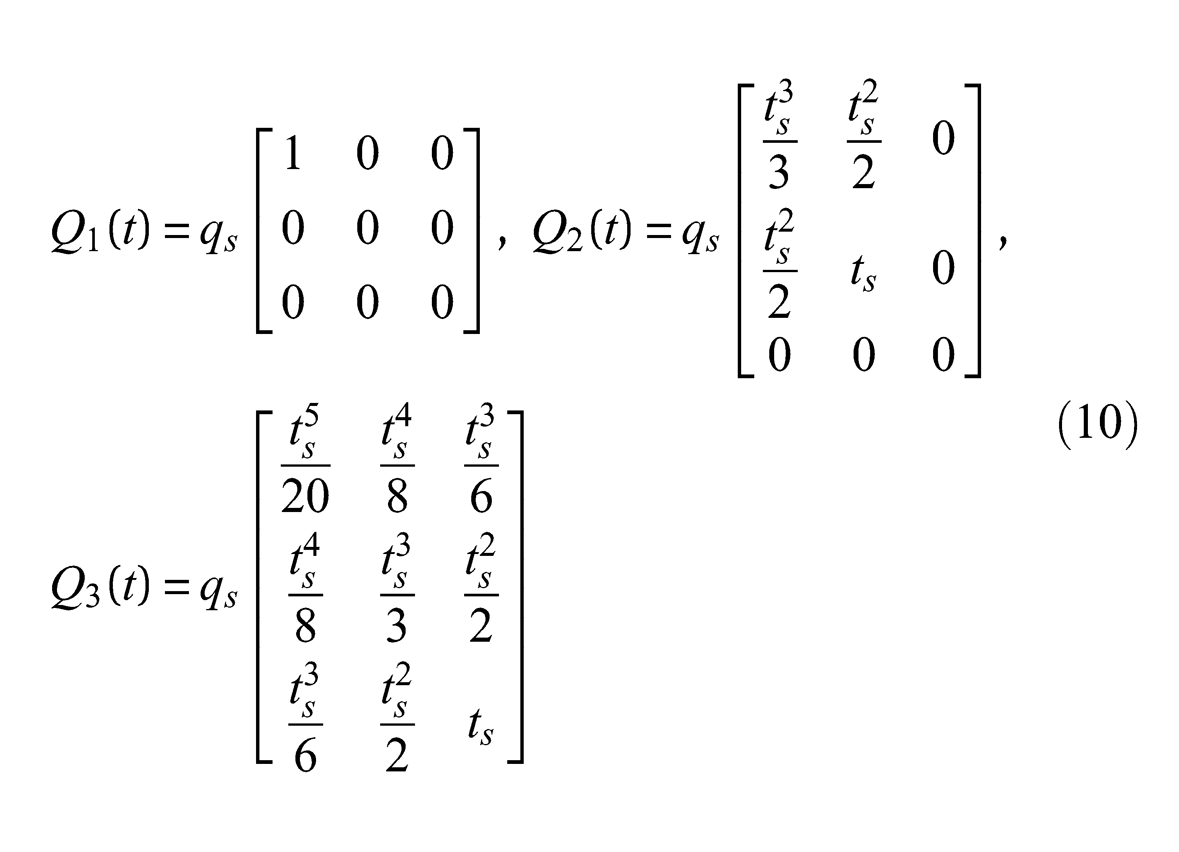
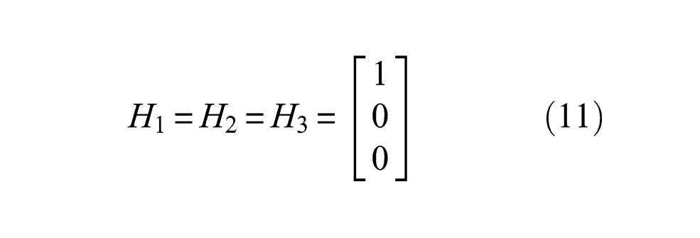
In this analysis, it is assumed that the bearing degradation is monotonically increasing and it evolves from normally operating to stable wear and then unstable wear. A linear, polynomial or exponential model is then used to describe the different trends in the vibration-based degradation signal of the bearing.4,27,28 These degradation processes are modeled using zero-, first-, and second-order KFs, respectively. For the unsteady degradation process, a second-order, quadratic function is adopted here as it can be described in a closed-form solution. Although an exponential function might describe the unstable degradation better, it will require nonlinear methods such as extended Kalman filter (EKF). 29 From Zarchan and Musoff, 11 the fundamental state, error covariance, and observation matrices describing the polynomial filter are shown below with subscripts 1, 2, 3 denoting the zero-, first-, and second-order KFs, respectively.
State matrices
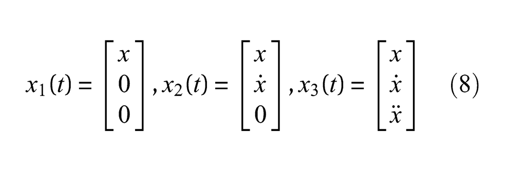
State transition matrices
Process error covariance matrices
Observation model matrices
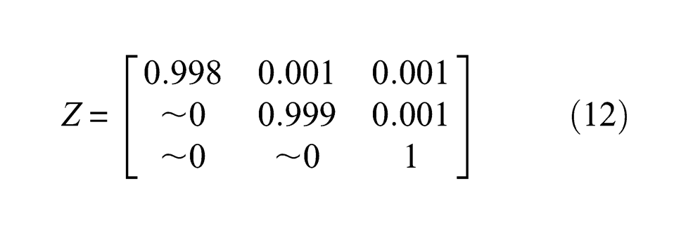
Model transition matrix
Initial model probabilities, state and covariance estimate
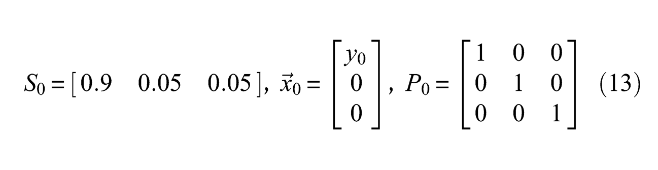
The state transition matrix Z is set such that the system tends to remain in its own state with Zii∼ 1. It is also assumed that the degradation rate can only progress, that is, from normal to stable and unstable wear but not the reverse. As such, Zij is assigned a value approximately 0 for i > j as a value of 0 can cause underflow problems in equation (4) when implemented as a software program. The measurement error, R, is obtained by taking the variance of the stationary measurements when the TRGB is in normal condition and this can vary between individual gearboxes. The assumption of stationary measurements from normal operating TRGBs in this study is validated based on measurements from several gearboxes. For TRGB 2, the measurement error, R, obtained is 3.2e−4. The initial model probability, S0, is set to a serviceable TRGB bearing with stationary CM measurement. The state estimate, x0, is initialized to the first measurement and an arbitrary covariance matrix, P0, is used.
Process error, qs
The process error, qs, contains the uncertainty of the filters in modeling the real world. 11 It is obtained by tuning the SKF model with past similar defect cases and is assumed to be the same across gearboxes. The SKF formulations are applied with qs set initially as a small percentage of the measurement error, R. The SKF model is then applied on the CM data from TRGB 1 and 3 and qs is tuned till the model is acceptably consistent yet responsive to changes in the degradation processes. With lower qs, the second-order filter will fit the measured data better compared to the first-order filter and the model becomes more sensitive to changes and also prone to over-fitting. Conversely, the first-order filter will fit better with higher qs and is less sensitive to changes. This means that a lower qs can detect unstable wear earlier, but this can be undesirable as second-order growth tends to overpredict RUL during initial stages.
In this study, a qs value of 5e−8 is obtained by tuning the model using TRGB 1 and 3 before being tested on TRGB 2. From Figures 7 and 8, it can be seen that the SKF can track the steady and unsteady degradation processes. However, it can be seen that the filter does not perform well when the CM data are not monotonously rising and the SKF then has to take a longer time before it converges. This may cause false alarms of unstable wear in practice and a way to reduce it is for maintainers to decide by evaluating the available model probabilities between stable and unstable wears. For example, a decision threshold may be designed such that unsteady degradation is considered only when the model probability is >0.95. As such, the unsteady degradation will only be triggered when the likelihood of the degradation model has converged. The drawback, however, is that lead time for RUL prediction may be reduced.
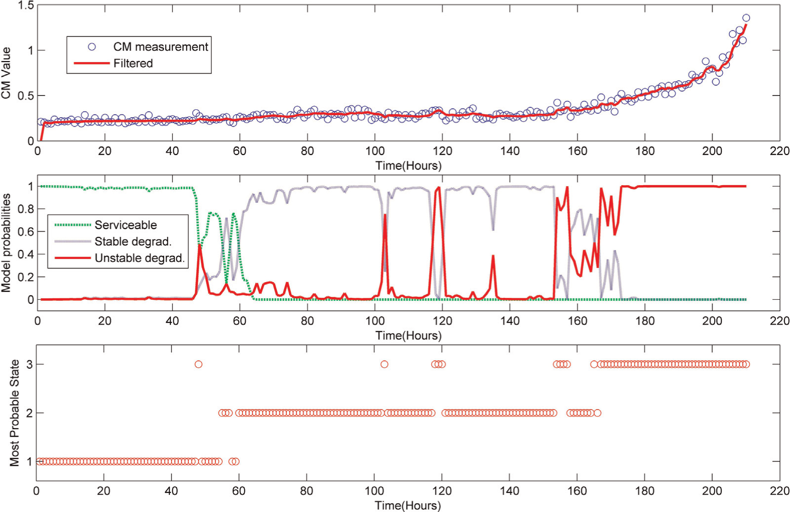
Top: plot of TRGB 1 CM measure and filtered value, middle: model probabilities, and bottom: most probable model with R = 4.3e−5, qs= 5e−8.
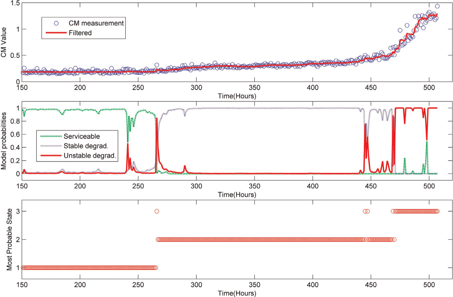
Top: plot of TRGB 3 CM measure and filtered value, middle: model probabilities, and bottom: most probable model with R= 6.2e−5, qs= 5e−8.
Diagnostic of bearing degradation
The formulated SKF model with the tuned process error, qs, is applied to TRGB 2 bearing CM data with a decision threshold of 0.95 used for unsteady degradation. The results are shown in Figure 9, and it can be seen that the SKF can adaptively track the different bearing degradation processes and provide the probabilities of each model at each time step. When compared to the optimal solution from the piecewise regression, the SKF transition time lags behind at 102 and 215 h compared to 87 and 202 h. However, it should be noted that the SKF is performing the estimation in real-time and requires adequate measurements from the dynamical process. At ∼120 and ∼200 h, the CM measurements are not increasing monotonically and the SKF has to obtain more subsequent measurements before it converges onto the degradation process. Figure 10 shows a comparison between the use of SKF and the use of a second-order KF. It can be seen that the SKF can better adapt to the different degradation processes and yield lower prediction errors compared to the use of a second-order KF alone, particularly in the normal condition. In steady degradation between 87 and 202 h, the prediction errors are comparable with RMS errors at 4.9e−4 and 4.7e−4 for SKF and EKF, respectively. SKF has slightly poorer results as predictions near transition point takes time to converge. In the time region away from the transition points between 110 and 190 h, the prediction RMS error for SKF was lower at 3.9e−4 against 4.4e−4 for EKF, respectively. Both the SKF and second-order KF yield the same results as the state progresses into unstable degradation.
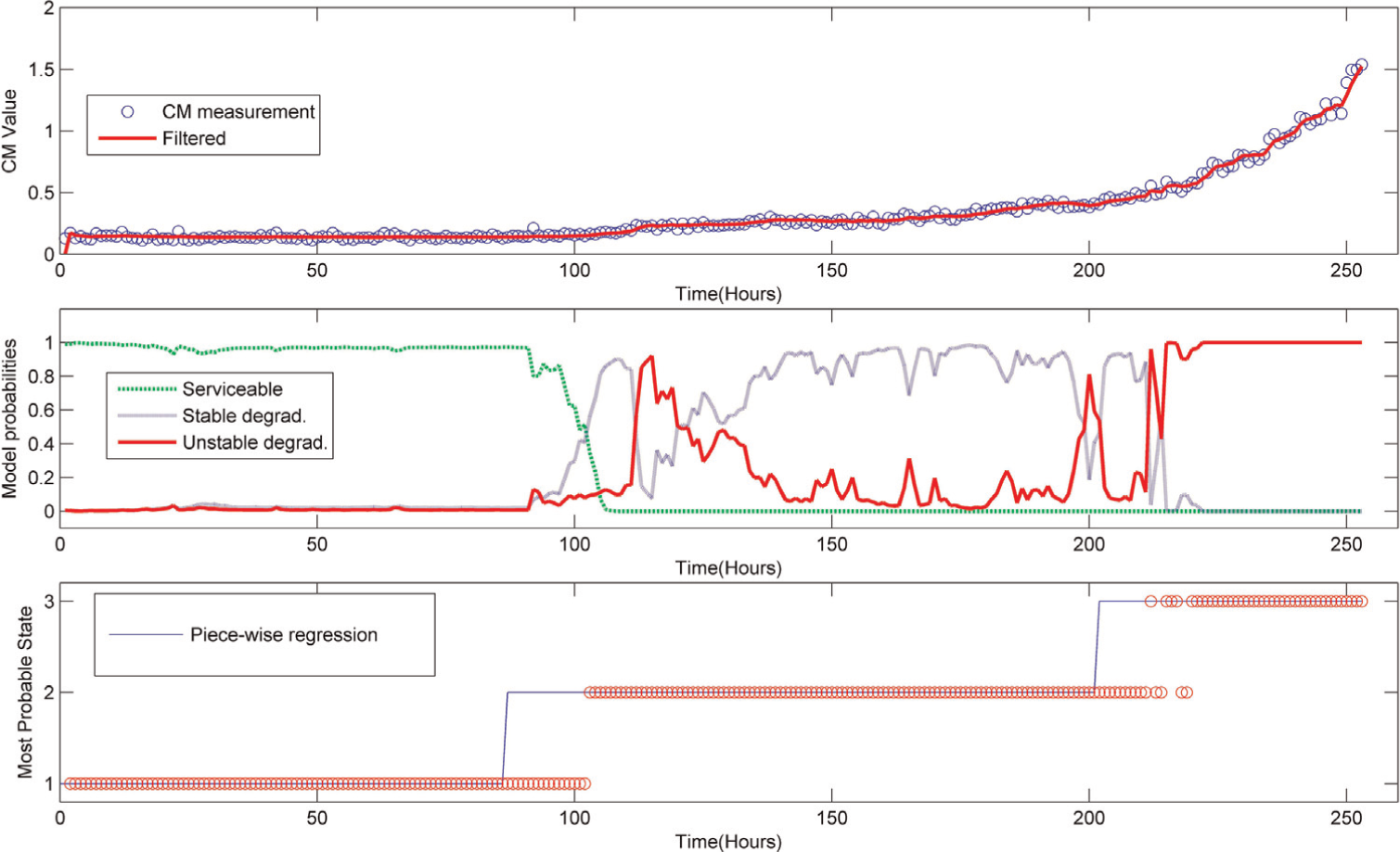
Top: plot of TRGB 2 CM measure and filtered value, middle: model probabilities, and bottom: most probable model with R= 3.2e−5, qs = 5e−8.
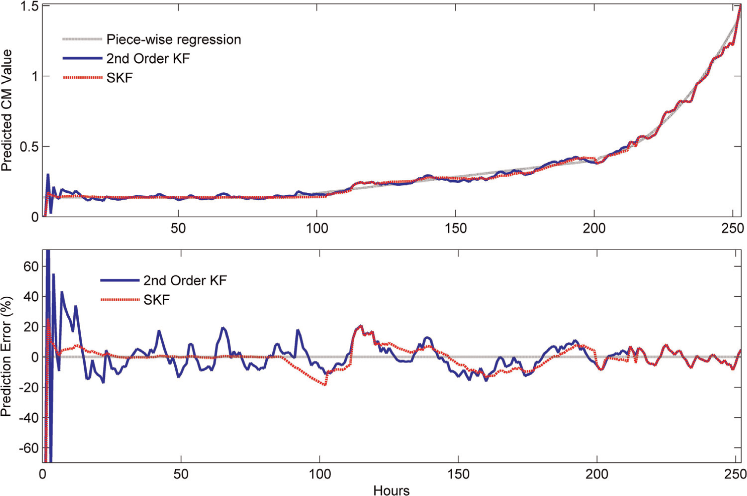
Top: comparison of predicted states using second-order KF with SKF and bottom: prediction errors of second-order KF and SKF from piecewise regression.
As mentioned earlier, the errors from the approximation using the GPB algorithm do not accumulate and the SKF will converge toward the underlying state. By using the SKF approach, the dynamical behavior between the current and past measurement is used to infer the degradation process and a detection threshold is not required. The CM data also do not need to be manually censored as the state for unsteady degradation can be triggered autonomously. Another key advantage of this approach is that it provides the probability of which degradation process the bearing is in. In comparison, the use of KF alone does not provide information on the degradation process as new measurements become available. The quantitative probability measure from the SKF allows more support for maintenance engineers as the probabilities of the bearing conditions can be compared in the event of outlier measurements.
Prognostic of bearing RUL
The RUL of the bearing is predicted only when unsteady degradation is detected as predictions from steady degradation are likely to be overestimated. The RUL is predicted by propagating the weighted state and covariance estimates obtained from equation (8) at each time step using equation (2) and determining the time when the degradation state crosses the failure threshold. The failure threshold has to be predefined and was established from the datasets available. Figure 11 shows the RUL forecast when the SKF detects unstable degradation after 215 and it can be seen that the accuracy of the RUL estimate improves as time progresses. However, the RUL prediction cannot be carried out at points where the state degradation rate,
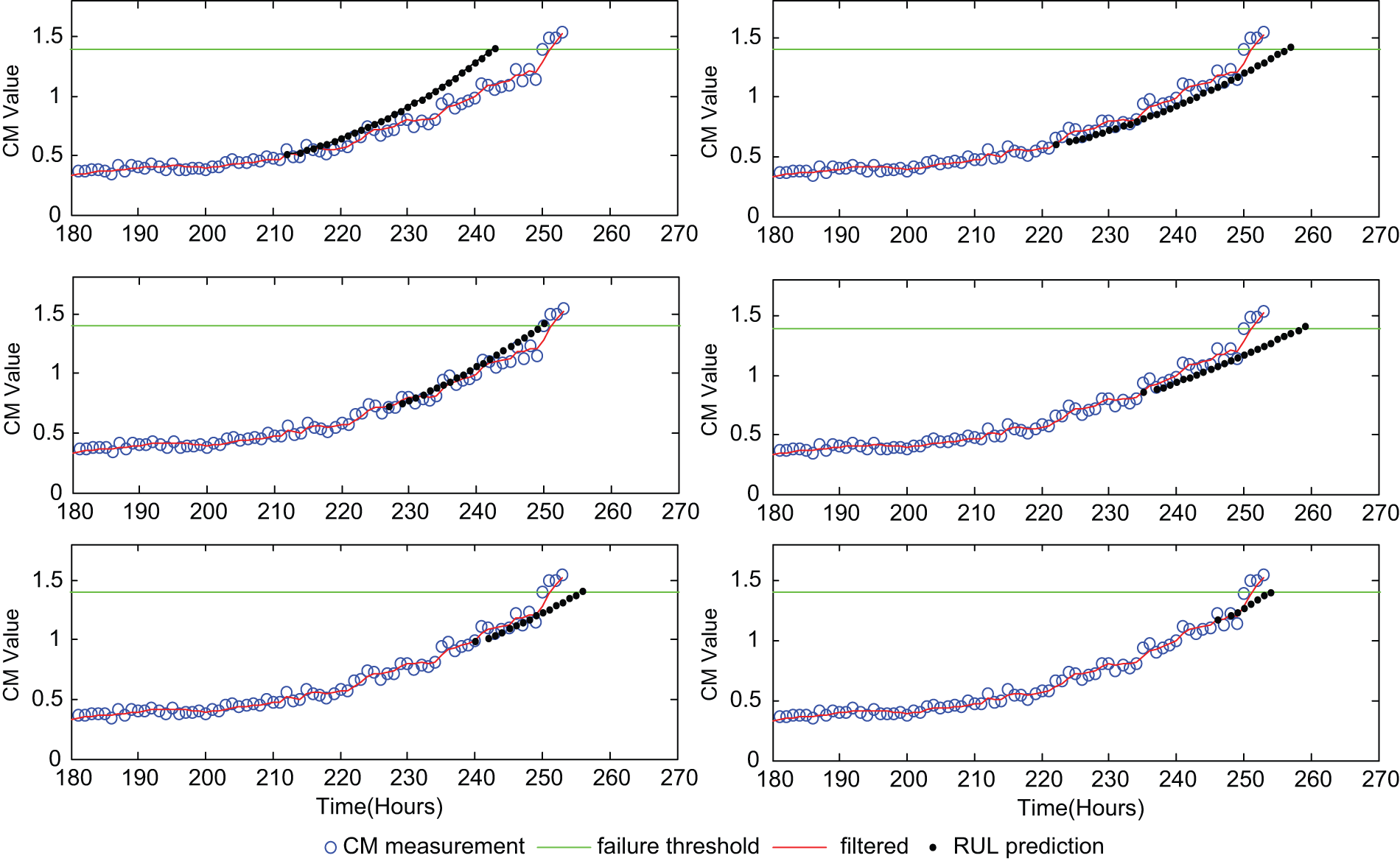
RUL forecast using SKF prediction at different times.
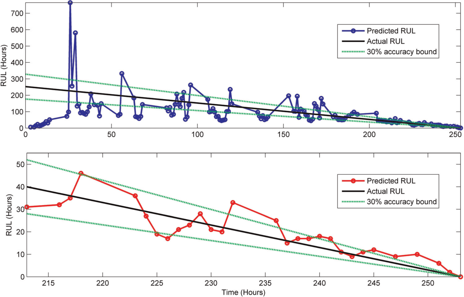
α-λ performance metric of RUL forecast using (top) second-order KF and (bottom) SKF.
The α-λ metric compares the actual RUL to the predicted RUL with converging α bounds that provide an accuracy region. The α bounds are application specific and a prediction is correct if it falls within the α bounds. From Figure 10, the prognostic algorithm performs well as its accuracy improves with time within the 30% bounds. As seen in Figure 12, the use of KF for prognostics alone will yield several predictions that fluctuate widely and are inaccurate during earlier stages of bearing wear. The RUL prediction stabilizes as it progress into unsteady degradation, but it will be difficult to determine when the prediction can be reliably used. With the SKF, the probability of unsteady degradation is known and the RUL can be adopted for maintenance planning.
Conclusion
In this study, the use of SKF in the diagnostics and prognostics of a helicopter gearbox bearing is presented with promising results. It is assumed that degradation process can evolve through time and the different degradation processes are modeled using a KF each. The SKF would then infer the underlying process accordingly and apply the most probable filter for RUL prediction. This approach can provide maintainers with more information for decision-making as a probabilistic measure of the bearing degradation process is available and allows prediction to be performed only when the degradation is unstable. A drawback of the current model is that prediction cannot be carried when the degradation rate,
Footnotes
Declaration of conflicting interests
The authors declare that there is no conflict of interest.
Funding
This research received no specific grant from any funding agency in the public, commercial, or not-for-profit sectors.