Field validation of controlled Monte Carlo data generation for statistical damage identification employing Mahalanobis squared distance

Abstract

This article presents the field applications and validations for the controlled Monte Carlo data generation scheme. This scheme was previously derived to assist the Mahalanobis squared distance–based damage identification method to cope with data-shortage problems which often cause inadequate data multinormality and unreliable identification outcome. To do so, real-vibration datasets from two actual civil engineering structures with such data (and identification) problems are selected as the test objects which are then shown to be in need of enhancement to consolidate their conditions. By utilizing the robust probability measures of the data condition indices in controlled Monte Carlo data generation and statistical sensitivity analysis of the Mahalanobis squared distance computational system, well-conditioned synthetic data generated by an optimal controlled Monte Carlo data generation configurations can be unbiasedly evaluated against those generated by other set-ups and against the original data. The analysis results reconfirm that controlled Monte Carlo data generation is able to overcome the shortage of observations, improve the data multinormality and enhance the reliability of the Mahalanobis squared distance–based damage identification method particularly with respect to false-positive errors. The results also highlight the dynamic structure of controlled Monte Carlo data generation that makes this scheme well adaptive to any type of input data with any (original) distributional condition.

Keywords

Statistical damage identification Mahalanobis squared distance controlled Monte Carlo data generation field validation multinormal sensitivity analysis

Introduction

The use of machine learning algorithms for practical structural health monitoring (SHM) in general and structural damage identification in particular has become increasingly popular in recent years. This is due to the fact that this approach could help overcome the adverse impact from inherent environmental and operational (E&O) factors that otherwise can prevent the intended objective such as structural damage from being detected.^1,2 To do so, a broad range of measured data collected under different E&O conditions of the structure is first used to train the learning algorithm. Once completed, the trained algorithm is supposed to understand the internal relationships of the data within each class (e.g. undamaged or at a specific level of damage) as well as to account for the underlying trend induced by E&O factors. Misjudgement induced from E&O impact can therefore be greatly mitigated, and the algorithm can be used to identify genuine structural damage. In this context, one of the most promising methods particularly in the unsupervised learning category is the use of statistical damage identification by means of the Mahalanobis squared distance (MSD)-based learning algorithm. In the more general disciplines such as novelty detection, the use of MSD-based learning algorithm is also very popular especially in the parametric statistical approach (as opposed to the non-parametric statistical approach).³ Compared to other popular damage identification methods such as those based on neural network, MSD-based method is generally more advantageous towards practical SHM systems which are often associated with the long-term and/or frequent data acquisition (DAQ) strategies. This is due to the architectural simplicity and computational efficiency of the MSD-based learning algorithm,⁴ making it more suited for dealing with large volume of data often encountered in such SHM systems in later monitoring stages. In recent experimental evaluations, MSD-based damage identification has also been among the most effective methods.^1,4–7 Besides its own application, MSD is also closely related to the popular Hotelling’s T² control chart and indeed equivalent to the T² statistic when the subgroup size is set at unity for the latter method.^2,8 In spite of having such wide connection and merits, the MSD-based damage identification method has, however, had one ‘Achilles heel’, that is, the requirement of the learning data to be multivariate normal (multinormal) distributed. This tends to be more problematic for the cases of employing the infrequent DAQ mode or at an early monitoring stage when not much measured data are available. To cope with this problem, the so-called controlled Monte Carlo data generation (CMCDG) scheme has been derived and reported in one of the recent publications of the present authors.⁹ Using this scheme, additional data can be produced from a limited number of original observations by means of an optimized Monte Carlo simulation process. Such an optimized simulation is useful not only to estimate an optimal noise level (which is to provide optimal randomness for the outcome data) but also to retain the (outcome) data at a reasonable size. Even though this scheme has been intensively tested against a sophisticated laboratory dataset, one may still be concerned that the success of using CMCDG has only been experimentally proved in a well-controlled testing environment. Additional applications towards real infrastructure vibration data are therefore in need in order to further evaluate and demonstrate the efficacy of this scheme.

To address this need and further extend the study on CMCDG, this article presents applications of this scheme onto real-vibration monitoring data from two actual civil engineering (one bridge and one building) structures each of which has been considered as an SHM benchmark structure. Of these two structures, the bridge can represent the case of having inadequate quality data and/or infrequent measurements, while the building represents the case where the data-shortage issue occurs at an early monitoring stage. To overcome such a data-shortage problem in either case, the CMCDG scheme is applied to the original learning data in order to generate well-conditioned synthetic data and therefore numerically stable (computational) system realizations. Besides utilizing two existing assessment indices in CMCDG, this study also employs statistical sensitivity analysis of the MSD computation using representative generated datasets to further validate the efficacy of CMCDG. The outcome of these applications reconfirms that the CMCDG scheme is able to help overcome the data-shortage problem and enhance the reliability of the MSD-based damage identification method. The layout of this article is as follows. The next section provides concise theoretical descriptions of the MSD-based damage identification method and the CMCDG scheme. The benchmark structures and their datasets used in this study are then briefly described. In the last two sections, detailed analyses and discussions are first provided before the key issues and findings are summarized in section ‘Summary and conclusion’. It might be worth noting that the scope of this research is currently restricted to Level 1 of the damage identification hierarchy, that is, to identify the presence of damage. However, as the problem of false indication has persisted fairly significantly at this level in the prior studies,^4,10 the present authors believe that enhancing the accuracy of this phase is still very crucial besides addressing problems of the higher damage identification levels.

Theory

MSD-based damage identification method

There are two main types of data used in a statistical damage identification process. In general, the primary (or raw) data acquired by sensors are not directly used but are transformed into a (damage sensitive) feature which then becomes the input data for the learning algorithm. Since this transformation process is often conducted by means of data compression methods such as modal analysis or time series modelling, feature data are often in a much lower dimension. The most popular features in SHM include the vectors of modal parameters or auto-regressive coefficients among others.

Suppose that a training feature dataset consists of p variables and n observations. If it approximates a multinormal distribution, this dataset can be represented by the sample mean vector $(\bar{x})$ and the sample covariance matrix (S). Next, each feature observation $(x_{i})$ for either training or testing purposes will be converted into a damage index in the form of distance (i.e. MSD) measure $(d_{i})$ as follows

d_{i} = {(x_{i} - \bar{x})}^{T} S^{- 1} (x_{i} - \bar{x})

(1)

Here, the mean and covariance are also the two representatives for the realization (of the MSD computational system) by the given dataset. This point is emphasized as there will be a large number of synthetic datasets (and therefore system realizations as well as their representatives) generated in the CMCDG process. In the damage identification context, the mean and covariance should be formulated as an exclusive measure, or in other words, consisting of no potential outlier from the testing phase.⁵ After computing all training distances, the assumption of a multinormal distribution again allows the estimation of the threshold from the basis of chi-square distribution for the training distances.² It is because under such an assumption, one can specify a statistical threshold for the distances based on a distribution quantile or equivalently a confidence level.^2,11 In the testing phase, whenever a new observation comes, its corresponding distance can then be used to compare against the threshold to determine whether it corresponds to a normal or damaged state. There might be a trade-off in choosing the confidence level: using a high level of confidence might not be able to detect a lightly damaged case that is known as one class of Type II errors but the least critical. However, such confidence levels can assist in avoiding as many as possible false-positive indication of damage (i.e. Type I errors).² In this study, one of such high levels (i.e. 99%) will be used in the application.

CMCDG

The CMCDG scheme proposed is an enhanced version of the conventional Monte Carlo data generation scheme which has been frequently used in the MSD-based damage identification context.^5,10,12 In both schemes, the shortage of data is compensated by the provision of statistical replications of each initial observation by means of Gaussian noise.⁹ However, the core components of the CMCDG scheme that make it more advanced than the conventional scheme are two data condition indices and a robust probability-based evaluation procedure used to obtain robust statistical measures for either index. Of the two indices, the (two-norm) condition number (COND) of the covariance matrix is intended to monitor potential computational instability associated with the use of the inverse of the matrix component in equation (1). On the other hand, the second index is the root-mean-square error (RMSE) between the theoretical and actual beta quantile–quantile (Q-Q) plots of each dataset generated during CMCDG process. By running a sufficiently large number of data generation simulations, the relationships between the commonly used robust probability measures (of either index) such as median and inter-quartile range (IQR); and the variable such as the noise level or the replication size can be constructed. The user is then able to use the convergence of these statistical measures to determine the optimal value for each of the two variables. The theoretical bases of the CMCDG scheme and the probability convergences of COND and beta Q-Q RMSE have been proved under the regulation of two well-known theorems, that is, central limit theorem (CLT) and the law of large numbers (LLN). Details of these can be found in the first article of the CMCDG scheme.⁹ Since its target is the enhancement of learning data multinormality, CMCDG can also be considered as a (multivariate) data normalization scheme with the focus on the Gaussian-type prerequisite for the learning process. Finally, although it has such desirable features, it should be noted that CMCDG might mainly be required by novelty detection methods (as well as associated damage identification methods) in the parametric statistical approach as these methods are often formulated from the multinormal data assumption.³ Methods from other approaches such as multivariate exponentially weighted moving average have been shown to have higher tolerance to non-multinormality and can therefore utilize simpler normalization schemes such as data shuffling to overcome the related impact.¹³

Description of the benchmark structures and their data status

Structural Monitoring and Control benchmark structure and data status

The first benchmark structure of interest is an actual cable-stayed bridge monitored by Center of Structural Monitoring and Control (SMC) at the Harbin Institute of Technology, China.¹⁴ Opened to traffic in December 1987, this is one of the first cable-stayed bridges in mainland China. This 11-m-width bridge consists of a main span of 260 m and two side spans of 25.15 + 99.85 m at each end. In 2005, after 19 years of operation, the bridge was found in a rather unsafe condition with a mid-span girder and a number of stay cables being cracked or corroded. Along with major rehabilitation programme undertaken to replace the damaged girder segment and all the stay cables, a sophisticated SHM system (see Figure 1) was implemented in order to monitor the bridge from the time of its rebirth in 2007. From monitoring data of this bridge, the SMC research group has been able to develop two SHM benchmark problems: one for stay cable condition assessment and the other for bridge girder damage identification. The context for the second benchmark problem whose data are used in this study is as follows. In August 2008, that is, only 8 months after the first complete DAQ after its rehabilitation, the bridge was again found in a new deficient structural condition with several new damage patterns in the girders. Fortunately, this bridge had been frequently monitored during this short period of time, and certain distinct difference in modal analysis results could be observed over this monitoring period. Sampled at 100 Hz, acceleration data of 12 days were split into hourly subsets and made available on the SMC website for participants of this benchmark study.¹⁴ In the study herein, only acceleration data recorded from 14 accelerometers installed on the deck are used. Part of this databank (i.e. of several first days) will be employed as the seed data to be input into CMCDG in order to achieve enhanced data for MSD-based learning process. Usable sets of the remaining data will be used for testing purposes. Details of these datasets are presented in the data analysis section.

Figure 1.

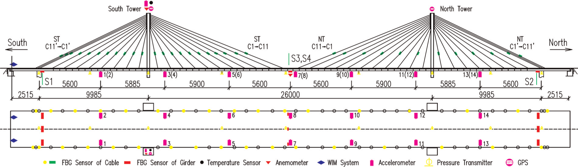
SMC benchmark structure.¹⁴

Queensland University of Technology–Structural Health Monitoring (QUT-SHM) benchmark structure and data status

The second benchmark structure used in this study is the main building with 10 main stories in the Science and Engineering Centre complex at the Gardens Point campus of Queensland University of Technology in Australia. The most notable feature of this benchmark structure lies at its vibration-sensing solution with a software-based synchronization method which can be seen as a promising alternative for use in vibration monitoring of civil infrastructure.¹⁵ At the lowest level of the system, there are only six analog tri-axial and two single-axis accelerometers available for use to capture the vibration responses of this structure. As illustrated in Figure 2, the sensors are located on the upper part of the building (i.e. at Levels 4, 6, 8 and 10) which is globally more sensitive to the ambient excitation sources such as human activities and wind loads. Acceleration data are sampled at the initial rate of 2000 Hz and then split into 30-min subsets for modal analysis purposes. In spite of using such a limited number of sensors, the sensing system could detect at least six modes with high confidence even under the challenging ambient excitation conditions. However, as the development of this sensing system has recently been completed, its databank is still limited with most of the data being collected during the system implementation phase in late 2013. Such limited data therefore need the assistance from a data generation scheme like CMCDG to enable the health-check process from an early stage. Details of the implementations of CMCDG onto the data of the two benchmark structures are presented in the next section.

Figure 2.

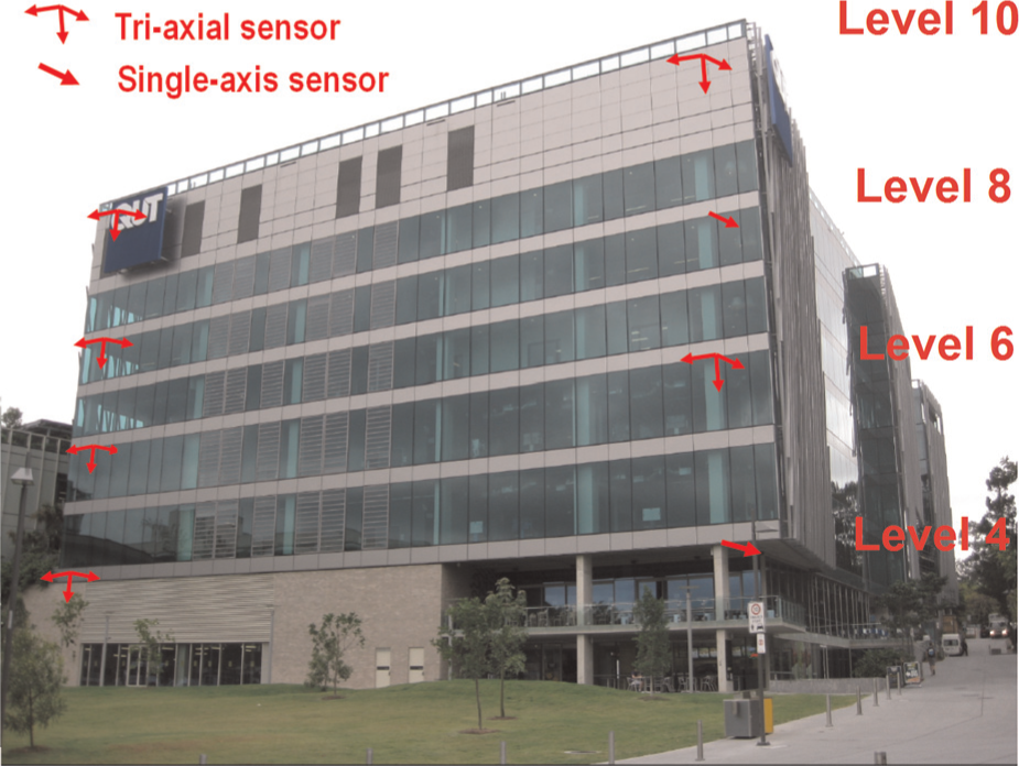
QUT-SHM benchmark structure.

Analyses and discussion

The feature selected for both benchmark study cases is the vector of modal frequencies estimated by means of the primary technique of the data-driven stochastic subspace identification (SSI-data) family (i.e. SSI-data employing unweighted principal component (UPC) estimator) in output-only modal analysis (OMA) approach. This selection is made due to the following reasons. First, modal frequencies can be more rapidly estimated with higher confidence than other modal parameters such as mode shapes.¹⁶ This is particularly meaningful for SHM in ambient excitation conditions where mode shape estimation is more challenging and time-consuming. Second, primary SSI-data are one of the most robust and advanced OMA techniques which can cope well with large volume of data from long-term SHM processes as well as vibration measurement uncertainties including data synchronization errors.^17,18 Third, online automated frequency estimation is highly possible in practice with the implementation of the recursive version of SSI-data.¹⁹ Finally, the modal frequency has been proved to be a main damage index at least for Level 1 of damage identification of several large-scale infrastructure such as the well-known Z24 highway bridge.²⁰

To process vibration data from two benchmark structures, the modal analysis software ARTeMIS Extractor Pro version 5.3 developed by Structural Vibration Solution A/S is used to implement the primary SSI-data technique. Concise descriptions of theory and usage for this technique can be found in several prior articles of the present authors.^17,18 SSI-data configurations and analysis results for each structure are presented in the following sub-sections.

SMC vibration data

For the sake of simplicity, the bridge is modelled, as illustrated in Figure 3, mainly with the main span (260 m) and the two larger side spans (99.85 m each) where 14 single-axis accelerometers were deployed. Checking across multiple datasets of this structure has revealed that one of these accelerometers (as circled in Figure 3) was out of order, but data from the remaining sensors are still adequate for modal validation (see the analyses below). Also, as they are found to be either mostly collected in poor excitation conditions or lacking in the stability along the consecutive sets, data from 3 days (31 May 2008; 7 and 16 June 2008) are excluded from the analyses. Besides these days, the problem of excitation has also had certain impact on the other days. Table 1 lists number of usable datasets from the selected 9 days. Descriptions of data grouping will be detailed below.

Figure 3.

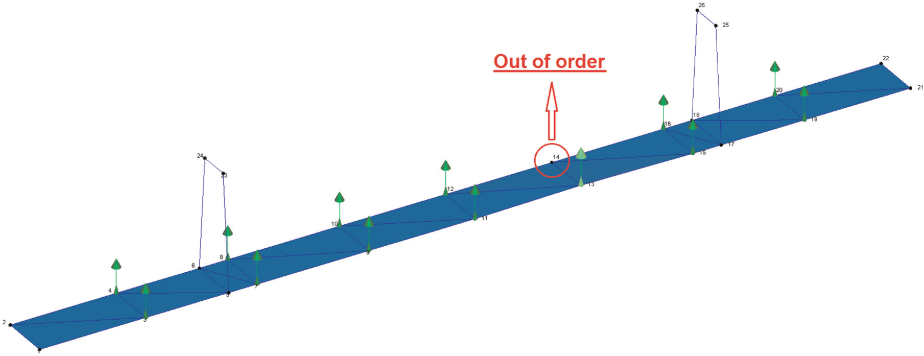
SMC bridge model in ARTeMIS Extractor software.

Table 1.

Selected testing days and usable datasets of SMC benchmark structure.

Selected testing day	Date^a	Number of usable subsets	Description of feature dataset
1	01 January	17	Days 1–3: Dataset 1 (State 1, 52 observations)
2	17 January	19
3	03 February	16
4	19 March	12	Days 4–8: Dataset 2 (State 1, 46 observations)
5	30 March	13
6	09 April	7
7	05 May	7
8	18 May	7
9	31 July	24	Dataset 3 (State 2, 24 observations)

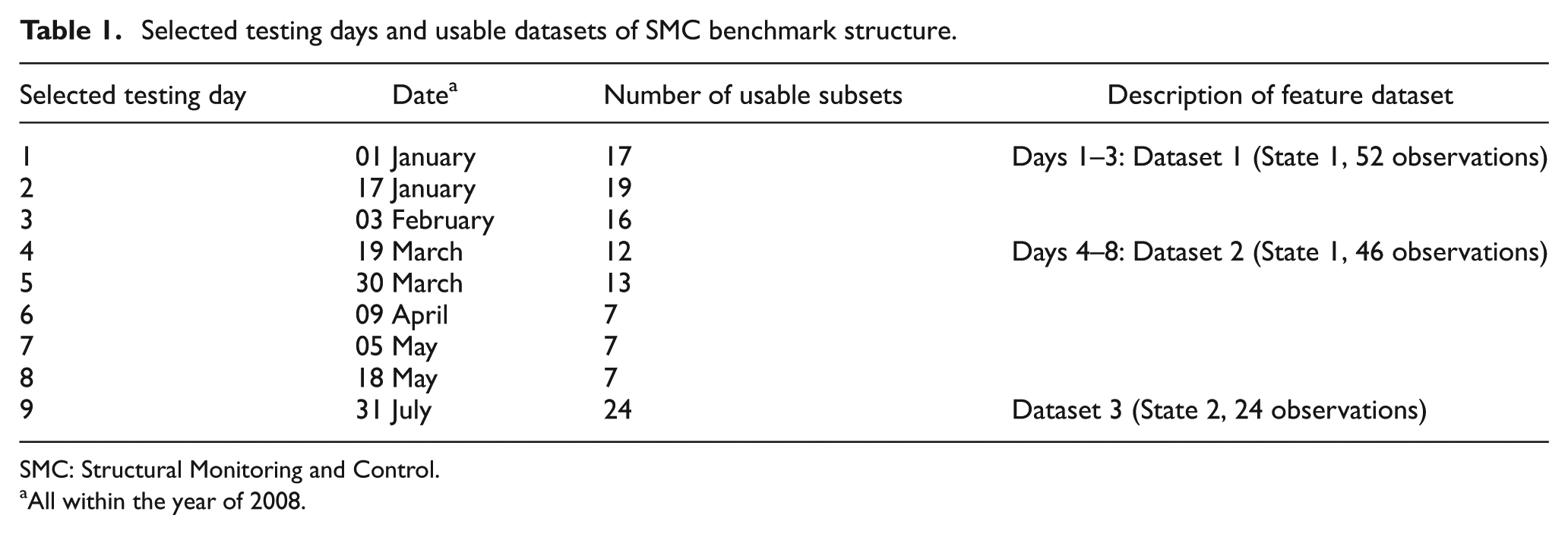
SMC: Structural Monitoring and Control.

All within the year of 2008.

The preliminary OMA by SMC group has pointed out certain differences between six frequencies (in the range of 0 to around 1.2 Hz) estimated from data collected in one of the first DAQ days (17 January 2008) and those from the data acquired in the last DAQ period (31 July 2008). These differences were assumed to be due to the impact of damage discovered in August 2008 as mentioned by Li et al.¹⁴ With a similar assumption, the following analyses in this section are to seek the evidence that the usable observations recorded during the first 8 days and the 9th day are likely to belong to two separate states, namely, States 1 and 2, respectively. To do so by means of the primary SSI-data technique, a frequency range of interest and a common modal analysis configuration are first required. Owing to small number of sensors and unidirectional measurement which hinder the validation of high-order modes, a decimation factor of 25 times is applied, and the frequency range of interest is restricted to between 0 and around 1 Hz to obtain the most accurate modal information. By comparing the results of SSI-data of incremental dimensions and projection channels, the most stable range of the maximum SSI state space dimension is found to be between 120 and 200, whereas that of the projection is from 8 to 11 channels. Hence, the maximum state space dimension of 160 and the option of 9 projection channels are first selected as the main SSI-data configuration for the vibration data subsets used herein.

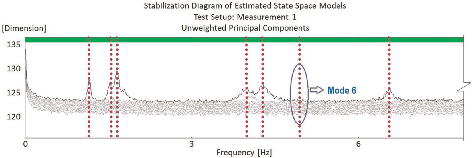
Using the above SSI-data configuration, around six modes may be detected and correlated between the two aforementioned states, and these can be illustrated in Figures 4 and 5 by using two representative datasets for these two states. Of these six modes, four (i.e. modes 1, 2, 5 and 6) consistently show up across all datasets of two states. The rather low value of the frequency magnitude of mode 5 in Figure 4(a) in comparison with Figure 4(b) is mostly due to the former corresponding to an extreme case (see below for detail of frequency comparison). On the other hand, modes 3 and 4, though consistently well detected in State 2, are only found weakly excited (Figure 4) in a limited number of datasets in State 1. This can be seen as the initial evidence for the difference between the two states. The corresponding mode shapes for the two datasets are presented in Figure 5 along with the corresponding modal assurance criterion (MAC) for each of the correlated mode shape pairs for the two states. It might be worth noting that all of the first five modes which exhibit a consistently increasing trend in MAC deviation belong to the vertical bending type, while mode 6 is of a vertical torsion. Compared to the Z24 highway bridge damage identification results,²⁰ low MAC values such as 0.83 and 0.62 (at modes 2 and 5, respectively) can also be seen as truly significant and can therefore serve as the second evidence for the difference between the two states. The last evidence for such a difference will be inferred from the statistical screening of frequency data in the succeeding paragraph.

Figure 4.

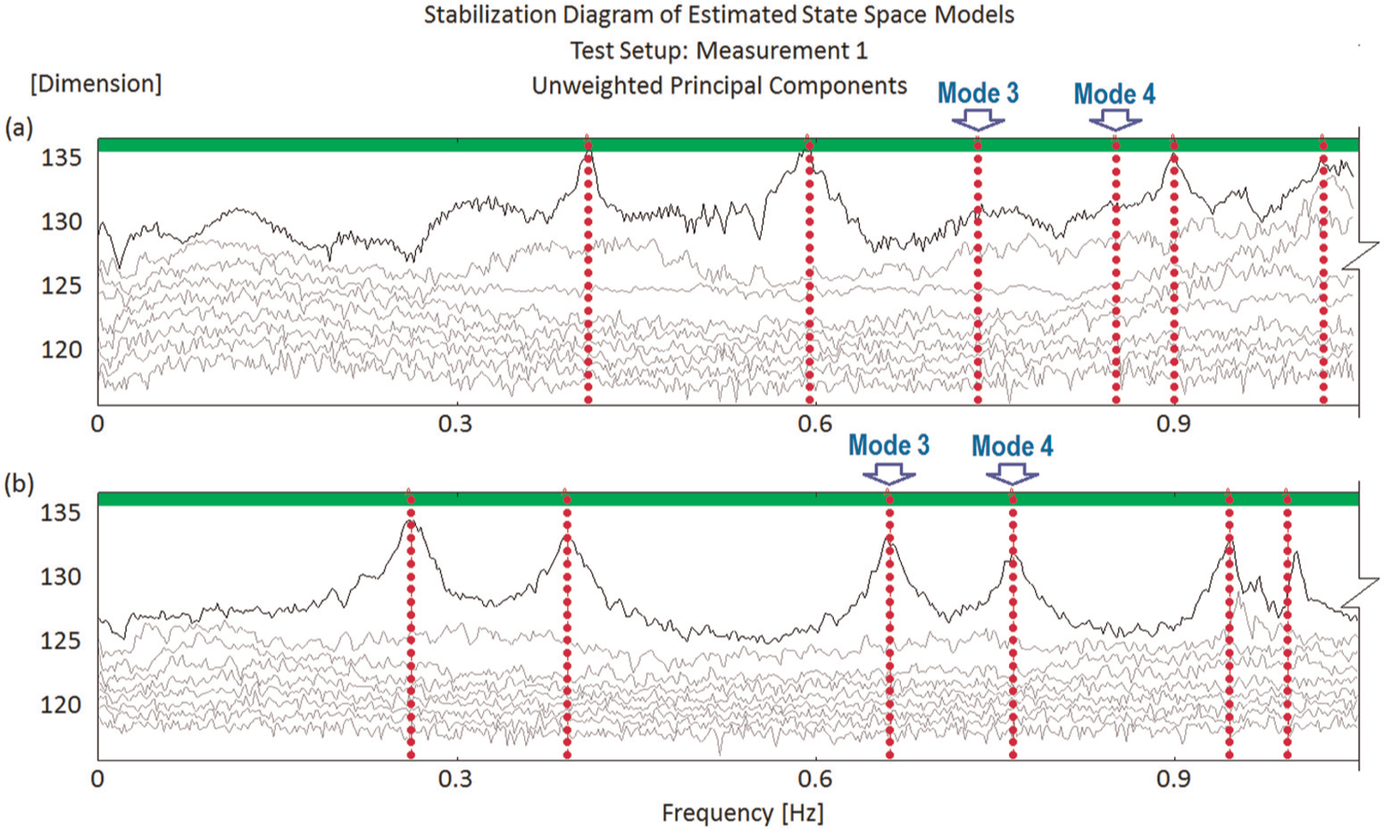
Detected modes of SMC benchmark structure: (a) State 1 and (b) State 2.

Figure 5.

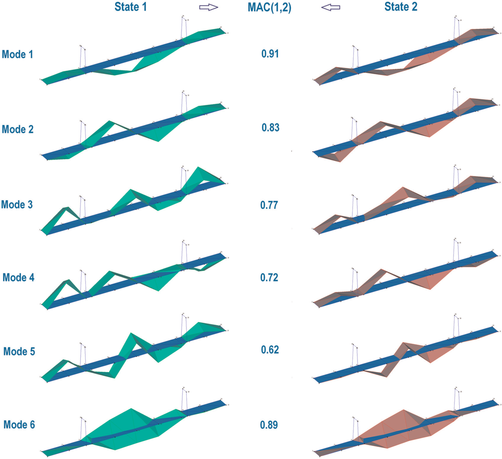
Representative correlation between (SMC) mode shapes of two states.

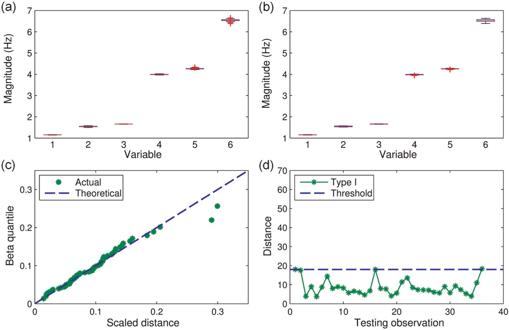
Owing to the absence of modes 3 and 4 in the analysis results from most datasets of State 1, the feature data could therefore be established from frequency estimates from the other four modes, or in other words, having four variables. For more detailed comparisons and validation of CMCDG later, feature data of State 1 are split into two sets, namely, datasets 1 and 2 with 52 and 46 observations, respectively (see Table 1 for more details). Figure 6(a) to (c) shows box plots of these two sets along with the third one (of State 2), and one can see that the datasets 1 and 2 are analogous to each other. On the other hand, dataset 3 possesses a distinct difference in the magnitudes of the first two variables. Even though the third variable experiences somewhat opposite change (compared to the other variables), the relative deviation at this variable is rather small (only +1.7%) compared to those at the two first variables (both almost −30%) in terms of their median values. A possible reason for the former symptom is that the modal frequency of this mode is insensitive to damage but slightly more sensitive to some E&O impact in a similar manner as occurred to the frequencies of the well-known I-40 bridge at its two first damage levels.^21,2 Nevertheless, the large reduction in the first two modal frequencies and the two prior evidences can be used as the bases to confirm the discrepancy between the two aforementioned states. Finally, it might be worth noting even though the use of frequencies and MAC values is satisfactory for damage occurrence confirmation herein, this type of damage detection methodologies is only convenient for the case with limited number of datasets. This is because, in this approach, the analyst would have to check every single feature dataset and compare with the others. For the case having many datasets such as in long-term and/or frequent SHM systems, this type of examination would become extremely time-consuming if not impossible. In this circumstance, the use of MSD-based damage identification is advantageous as it can run autonomously computing the testing distance whenever a new feature observation is available, comparing with threshold and (if larger) giving alarm in a fully automatic manner. Such operation and evaluation capacities of the MSD-based method are critical in order to ensure timely intervention and decision-making towards civil infrastructure and to constantly safeguard the users involved.

Figure 6.

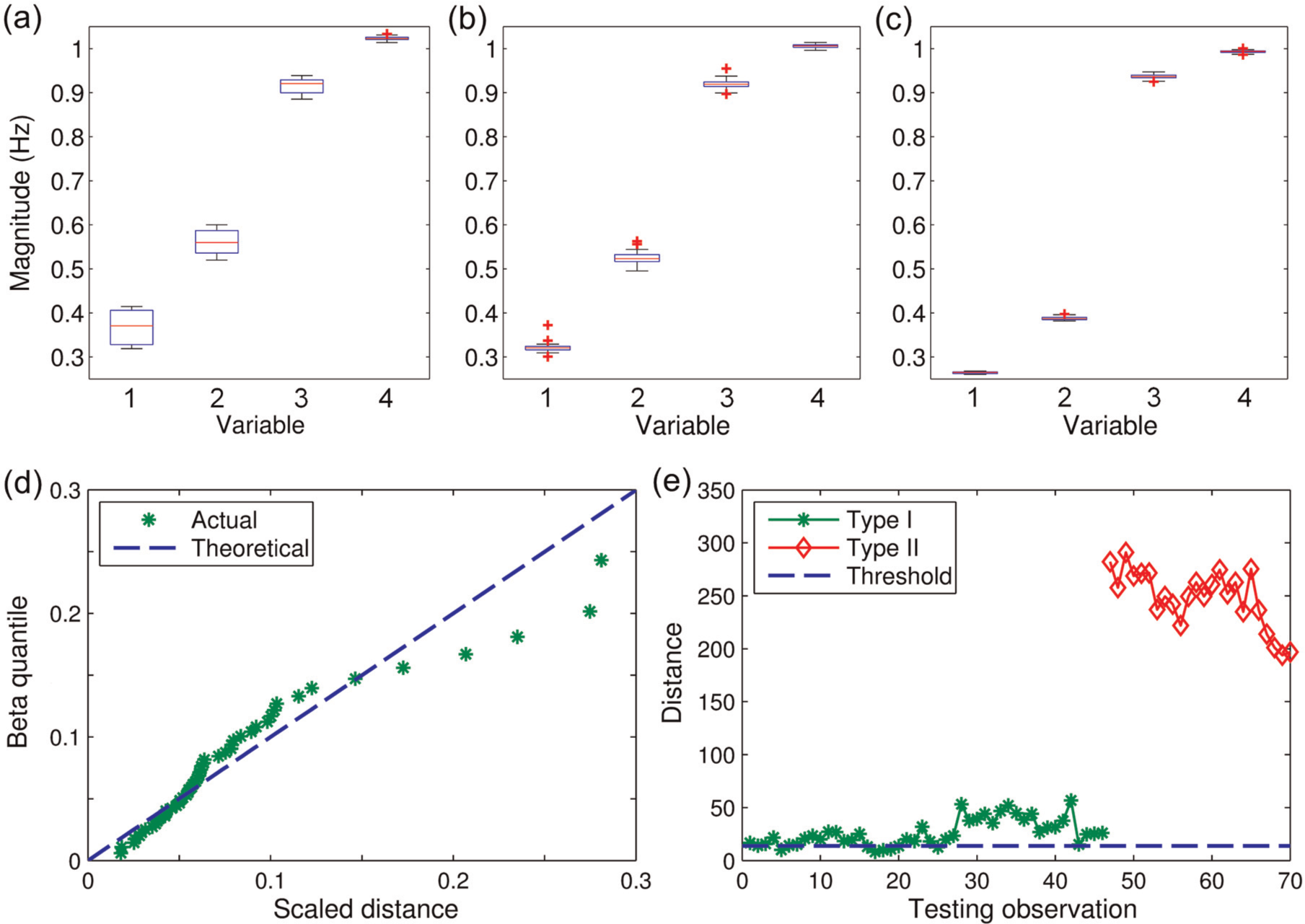
Characteristics of SMC data and original testing results: (a) and (b) datasets 1 and 2 (State 1), (c) dataset 3 (State 2), (d) beta Q-Q plot of dataset 1 and (e) original testing results.

In order to rigorously examine the efficacy of a method in distinguishing any two known structural states, the problem should be formulated in the context of hypothesis testing with two hypotheses known as the null hypothesis (H₀) and the alternate hypothesis (H₁). In the damage identification context, the null hypothesis is often assumed for the case when damage is not present, while the alternative hypothesis asserts the contrary.² In a probabilistic sense, two kinds of errors may be encountered when testing these hypotheses. If the null hypothesis is rejected even though it is true, then a Type I (false-positive) error has occurred. In contrast, if the null hypothesis is accepted even though it is false, then a Type II (false-negative) error has been committed. In a comprehensive hypothesis testing programme, the probabilities of these two error types can then be estimated based on a data distribution under assumption.²² However, for the purpose of simplicity, no probability computation will be made, and the assessment process herein will be conducted based merely on direct comparison of the error quantities to evaluate the efficacy of CMCDG in assisting the MSD-based damage identification method. Hence, dataset 1 will be used as the original learning data, while datasets 2 and 3 will be employed for the Type I and Type II error-testing purposes, respectively.

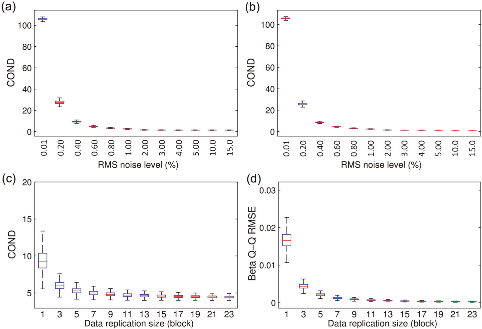
To check the degree of multinormality of the original learning data, the beta Q-Q plot is employed, and the result is shown in Figure 6(d), and one can see that there is a poor agreement between the theoretical and actual lines. This means that the original learning dataset has rather poor multinormality and therefore needs to be enhanced before it can be used for novelty detection or damage identification purposes. As a blind attempt to use this low-quality dataset, the MSD-based damage identification process is implemented onto the 70 (i.e. 46 for Type I and 24 for Type II) testing observations, and the testing results are presented in Figure 6(e). A closer look for the (selective) Type I distances in conjunction with the threshold can be seen in Figure 9. While no single Type II error is found, Type I errors are extremely severe with more than 80% false indications (as shown in Figure 6(e) with most Type I data points lying above the threshold line). To enhance the initial learning data by CMCDG, the optimal Gaussian noise level in the root-mean-square (RMS) sense is first determined by box-plotting COND of the datasets generated in each data generation set-up and tracking the convergence of the median or IQR for multiple set-ups. Figure 7(a) and (b) shows two of such plots of COND at different noise levels (from 0.1% to 25%) when running 10,000 simulations for the first CMCDG round with two illustrative cases, that is, to generate 9 and 18 additional blocks of data replication. Note that three different incremental levels of noise (i.e. 0.3%, 1% and 5%) are used in Figure 7(a) and (b) in order to facilitate better displays in different ranges of noise.

Figure 7.

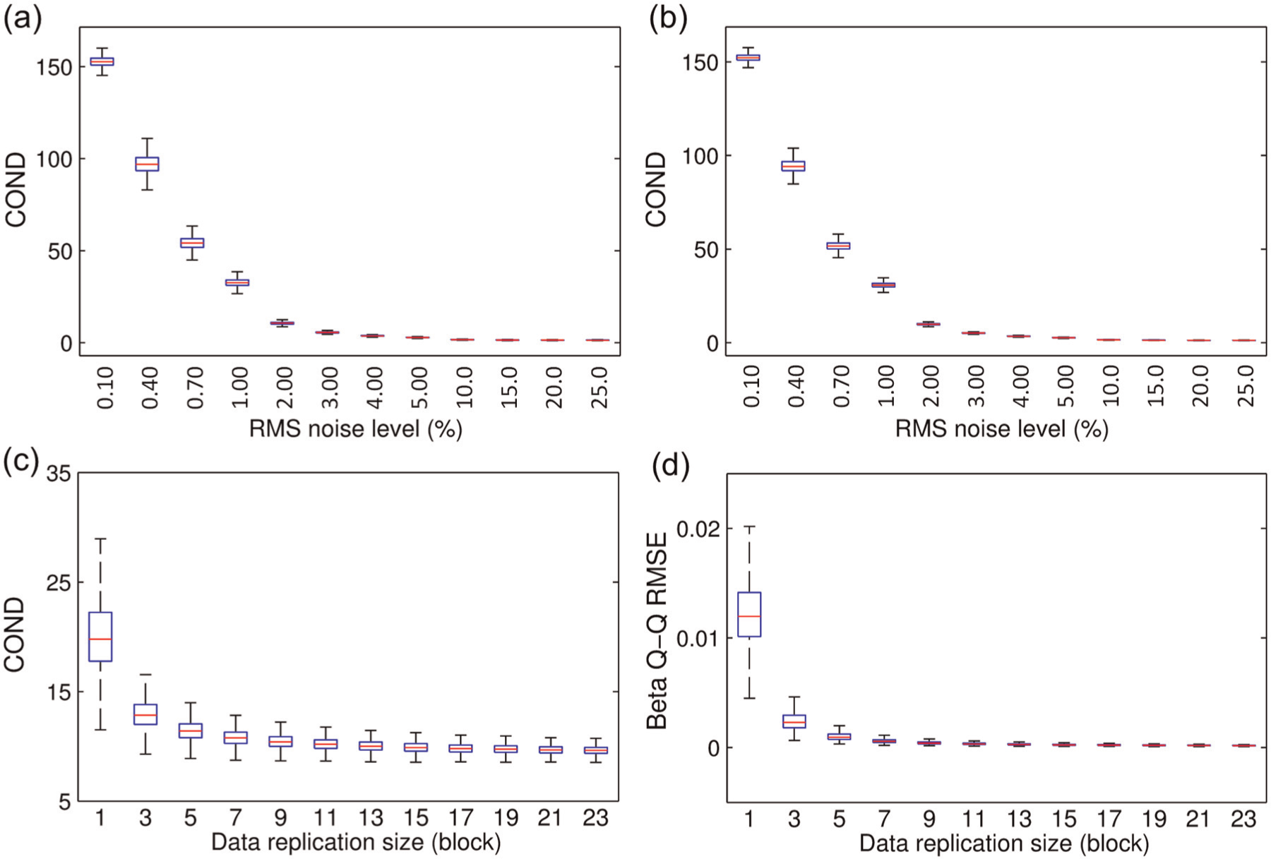
Results of two simulation rounds in CMCDG for SMC data: (a) and (b) round 1 with COND of 9 and 18 replication blocks; (c) and (d) round 2 with COND and beta Q-Q RMSE at noise level of 2%.

As can be seen from Figure 7(a) and (b), COND values become significantly small and steady after increasing the noise amount by several small steps and become essentially unchanged at the noise level of 20%. For ease of the selection of an appropriate noise level that corresponds to an essentially small COND (as this level might vary significantly from case to case as to be seen below), the so-called 95% deviation bounds criterion is established as follows. A COND value is considered as essentially small if its deviation from the original COND (i.e. of the original learning dataset) is no less than 95% of the COND span. Here, the COND span is the difference between the original COND and the COND value that has been considered essentially unchanged, that is, corresponding to the noise level of 20% in this case. Applying this criterion upon the medians of COND herein, the appropriate noise levels are found to be from 2% onward. Therefore, the optimal noise level is set at this starting point since the use of higher noise levels tend to reduce the sensitivity in detecting lightly damaged states as noted in the initial investigation with CMCDG.⁹ Employing this noise level, the second round of simulations is operated with the variable being the data replication size and the output being COND and beta Q-Q RMSE. These two results are graphically shown in Figure 7(c) and (d). From this figure, one can find again that COND and beta Q-Q RMSE become significantly small and steady from the replication size of around 9 blocks onward. This figure is therefore considered optimal replication size to provide quality synthetic datasets.

Using this optimal replication size, well-conditioned synthetic data can be generated with the previously selected optimal noise level (2%). Figure 8 shows the beta Q-Q plot and the hypothesis testing results for a typical one of such datasets when using it as a replacement for the low-quality original learning data (i.e. dataset 1). Note that the Type I and Type II error-testing data are kept the same as earlier (i.e. datasets 2 and 3 with 46 and 24 observations, respectively). Compared to original results reported in Figure 6(d) and (e), substantial improvement in beta multinormality degree is undeniable as reflected in Figure 8(a), while all the testing observations are accurately identified with no single error in both testing cases as seen in Figure 8(b). The enhanced learning data have well improved the reliability of MSD-based method with respect to the Type I error tests while being able to retain sufficient sensitivity to all Type II error-testing observations.

Figure 8.

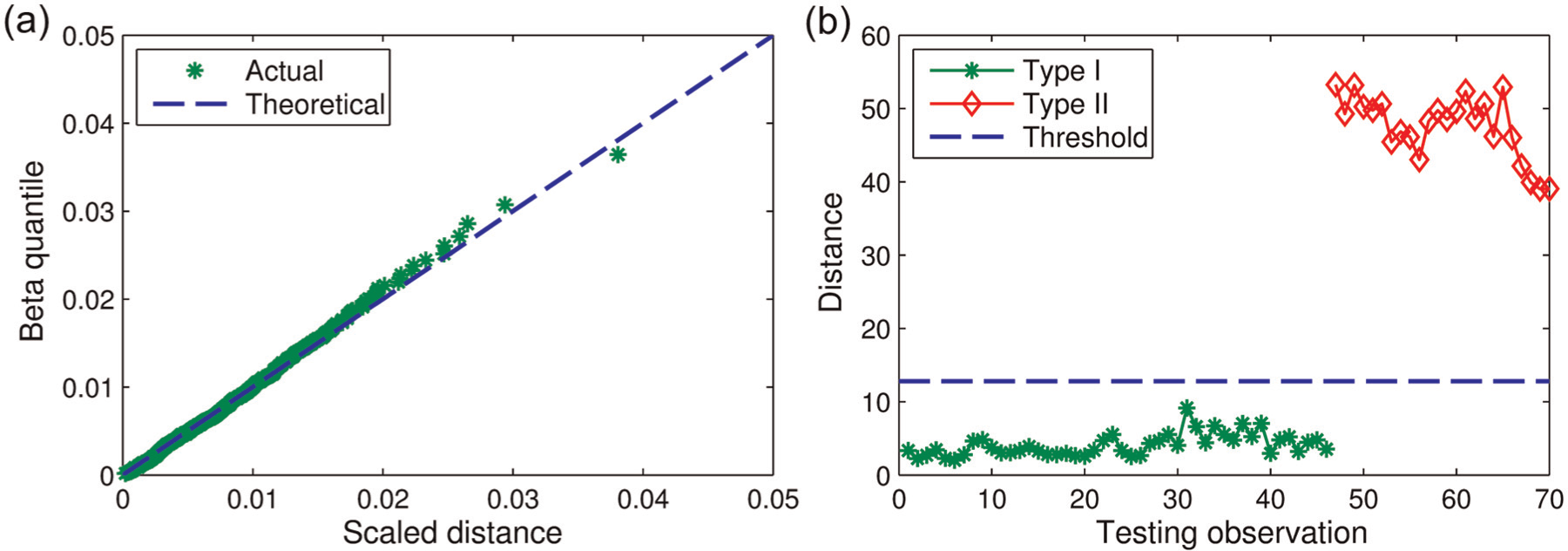
(a) Beta Q-Q plot and (b) testing results for a typical enhanced (SMC) learning dataset.

The earlier problem of having severe Type I errors in the original learning dataset (Figure 6) is believed to originate from the instability of the realization (of the MSD computational system) corresponding to this dataset. This has been actually reflected through comparison of COND (in Figure 7) since system realizations with larger COND values tend to suffer from more severe computational instability as previously mentioned. To illustrate this in a more direct manner in MSD-based damage identification process, the robustness of the original computation system realization (i.e. by original learning dataset) with respect to the perturbation of the Type I error-testing observation will be assessed against that of the realization by the (typical) enhanced dataset shown in Figure 8. Note that this type of assessment is commonly known as sensitivity analysis which is often used to test the robustness of a mathematical model or system in the presence of input uncertainties.^23,24 Projecting this onto the problem herein, the desired realization (by an appropriate dataset) of the MSD computation system should be as robust as possible against the presence of inherent perturbation (of the testing observation) that may be induced from measurement or data compression phases. Based on this fact, the aforementioned comparative assessments between the original and enhanced datasets are objectively realized by means of the same input (i.e. each of 46 Type I error-testing observations); the same magnitude of its statistical perturbation; and once again the Monte Carlo simulation in a similar fashion that is used in CMCDG. Specifically, the perturbation level is selected as 2% with respect to the RMS of each investigated observation. Then, 10,000 simulation rounds for the perturbation application and the MSD computation are operated, and the corresponding original testing distance and its (10,000) variants are box-plotted in Figure 9 for the both original and typical enhanced datasets. Note that due to the paper display limitation, only 12 selective cases (out of a total of 46 testing observations) are reported in this figure for either dataset. Compared to those obtained from the typical enhanced dataset, the fluctuations of the Type I distances computed from the original dataset are significantly (i.e. 10 to 15 times) larger. Furthermore, compared to the magnitude of the threshold, these fluctuations are also truly severe as seen in Figure 9(a). Such large fluctuations indicate that it is highly likely that the realization of MSD computational system by the original dataset is in a significantly ill condition, and the computational results are unreliable. On the other hand, the marginal fluctuations in Figure 9(b) show that the robustness of the computational system has been considerably enhanced through the use of a dataset generated from an optimal CMCDG configuration. Further checks with other datasets generated by succeeding CMCDG configurations have confirmed the robustness convergence for this configuration, but the detailed results are not shown to save space.

Figure 9.

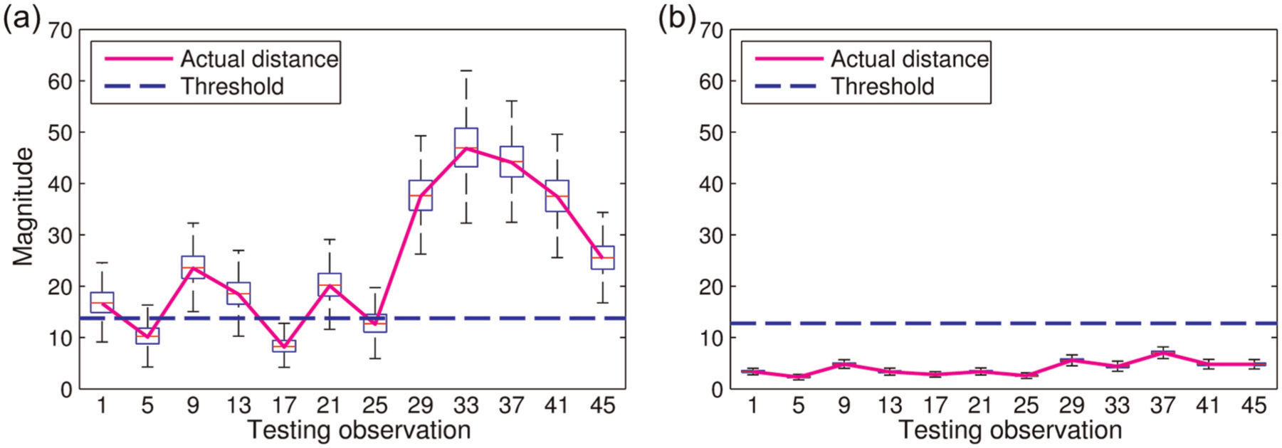
Impact of input perturbation on (SMC) MSD computation: (a) original learning dataset and (b) typical enhanced learning dataset.

QUT-SHM vibration data

As mentioned earlier, as the full monitoring programme for this benchmark structure has recently been started, its databank is still limited with 100 subsets at the time of processing data for this article. Of these subsets, most (64 subsets) were collected during the system development phase in late 2013, and the remaining (36 subsets) were collected in January 2014. Using an optimal SSI-data configuration similar to the one used for the SMC data, up to seven modes could be estimated as illustrated in Figure 10 for one representative data subset. Nevertheless, only six of the modes (i.e. modes 1–5 and 7 as typically animated in Figure 11) are usable for the purpose of continuous modal tracking. The exclusion of mode 6 is due to the inconsistency of modal estimation at this particular mode across different datasets recorded under different E&O conditions. As it is a weakly excited mode (i.e. not corresponding to an obvious peak as seen in Figure 10), mode 6 can be only properly estimated when the signal quality is in fairly good condition. To implement the hypothesis testing, the modal frequency data (of the six usable modes) obtained from the two aforementioned portions of the QUT-SHM databank are used to establish the original learning and testing datasets with 64 and 32 observations, respectively. The box plots of these two datasets, as presented in Figure 12(a) and (b), first show that their magnitude distributions are in excellent agreement with each other. Another supporting evidence is that the mode shape agreement across the two sets is very high with MAC values being frequently higher than 0.9. It is therefore sensible to assume that these two datasets belong to only one structural state. Since no data from another structural state are available with this newly constructed building, the hypothesis testing is restricted merely to the Type I error tests.

Figure 10.

Detected modes of QUT-SHM benchmark structure.

Figure 11.

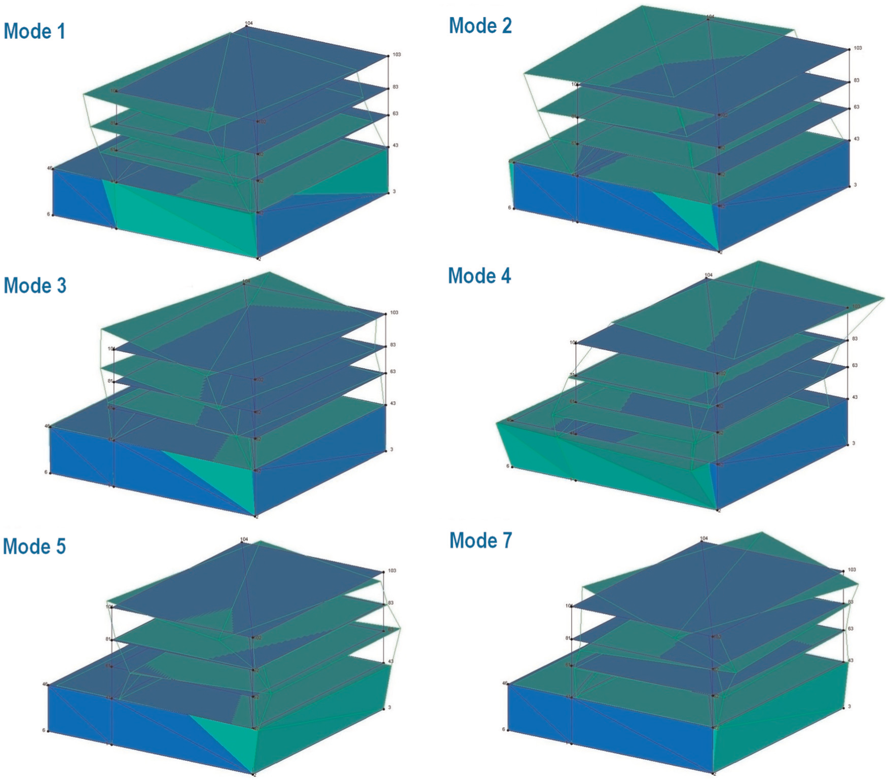
Mode shapes of six usable modes of QUT-SHM benchmark structure.

Figure 12.

Characteristics of QUT-SHM data and original testing results: (a) original learning dataset, (b) testing dataset, (c) beta Q-Q plot of original learning dataset and (d) original testing results.

Using the same investigation procedure that has been done for the SMC data, the beta Q-Q plot of the original learning data and the Type I testing are conducted for the QUT-SHM data, and the results are shown in Figure 12(c) and (d). One can see that the agreement between the actual beta Q-Q plot and the theoretical line in this case is slightly better than that of the SMC data. This is reflected by the fact that most of data points in Figure 12(c) stay closer to the theoretical line than those data points of the SMC case presented in Figure 6(d). The Type I error still comes across, but the rate is significantly smaller (than that of the SMC case) with just over 10% false-positive detection as illustrated in Figure 12(d). To see whether CMCDG could further improve this situation, the same simulation process as for the SMC data is conducted, and the results of two simulation rounds in CMCDG are reported in Figure 13. Applying again the previous criterion of 95% deviation bounds, the optimal noise level is found at 0.6%, and the convergence trends around this level are illustrated in Figure 13(a) and (b) for the two replication sizes of 7 and 14 blocks, respectively. Employing this noise level and tracking the convergence of both COND and beta Q-Q RMSE from Figure 13(c) and (d), one can again select the optimal replication size at 9 blocks. Compared to the optimal noise level (2%) of the SMC data, the optimal level in this case is considerably smaller, and a possible reason for this symptom is that the original QUT-SHM learning dataset has better multinormality than that of the SMC bridge structure. This has in fact been reflected through the previous comparison of multinormality degrees (based on the beta Q-Q plots) between two original datasets of the two cases.

Figure 13.

Results of two simulation rounds in CMCDG for QUT-SHM data: (a) and (b) round 1 with COND for 7 and 14 replication block cases; (c) and (d) round 2 with COND and beta Q-Q RMSE at noise level of 0.6%.

For further checking purposes, well-conditioned synthetic datasets are generated by the optimal CMCDG configuration (i.e. noise level of 0.6% and replication size of 9 blocks) previously estimated. Figure 14 shows the beta Q-Q plot and the Type I error-testing result for a typical one of such datasets, while Figure 15 reports the impact of input perturbation on Type I distance computation based on the same sensitivity analysis procedure as previously conducted for the SMC data. For the latter figure, 12 of the testing observations (i.e. one of every three) are selected to fit the paper display space. Once again, improvement can be found for both multinormality and Type I error-testing results, while the stability of the computational system has been typically improved by 6–10 times by the data optimally enhanced by CMCDG. These results reconfirm the efficacy of the CMCDG scheme in enhancing the condition of learning data and the corresponding computational system realization so that more reliable damage identification outcome can be achieved. Besides, since there is no significant change in the magnitudes of the thresholds between the original learning data and the enhanced data (Figures 9 and 15) in both SMC and QUT-SHM data cases, it can be concluded again that CMCDG does not significantly change the magnitude of feature data as noted in the initial study of this scheme.⁹ Instead, its effectiveness has mainly come from the provision of additional observations which are randomly distributed against the original data as led by CLT and LLN theorems, and this has been reflected through the irrefutable convergence trends of both COND and beta Q-Q RMSE as previously shown. With the successful applications in two real civil engineering structures herein, the CMCDG scheme can be considered to be successfully validated by field test data.

Figure 14.

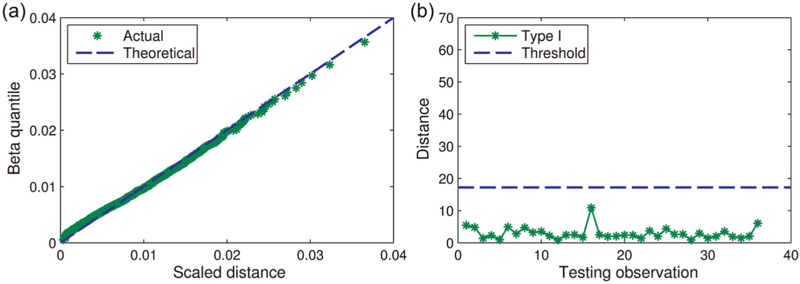
(a) Beta Q-Q plot and (b) testing results for a typical enhanced (QUT-SHM) learning dataset.

Figure 15.

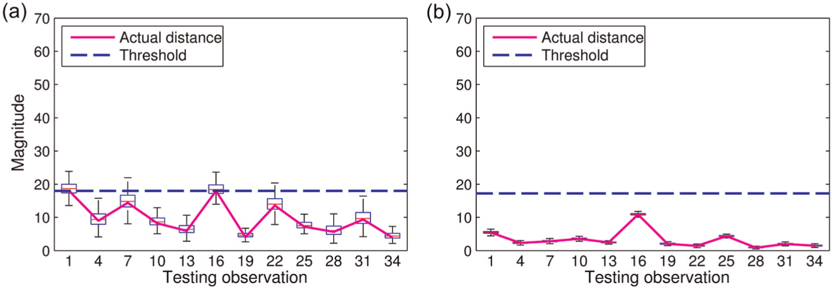
Impact of input perturbation on (QUT-SHM) MSD computation: (a) original learning dataset and (b) typical enhanced learning dataset.

Summary and conclusion

This article has presented the field applications and validations for the CMCDG scheme recently derived to assist the MSD-based damage identification method to cope with the problem of data shortage which can cause inadequate data multinormality and unstable MSD computation. To do so, two benchmark SHM structures are used in which the bridge represents the case of having infrequent and/or inadequate quality measurements, while the building represents the case where the data-shortage problem occurs at an early monitoring stage. Owing to limited availability of actual observations, the original learning dataset of either case has been revealed to be in such poor multinormal distributions that require the data to be enhanced before it can be reliably used for the MSD-based damage identification process. It has also been shown that a blind attempt to use these low-quality data may result in a significant rate of false-positive errors, and the severity of this type of errors tends to be proportionate to the poorness of the data multinormality. However, with the enhancement from CMCDG, these problems have been shown to be effectively mitigated. Under optimal data generation configurations derived in CMCDG, well-conditioned synthetic data for the learning process has been generated with remarkable improvements in multinormality degree as well as MSD computational stability. The latter has been critically assessed not only by comparisons with each original (low-quality) dataset via COND as in the original work in CMCDG but also with respect to the consequent impact of using such a dataset on the testing results. The ultimate outcome of the applications of CMCDG to the field data herein has reconfirmed that CMCDG is able to overcome the poor data multinormality problem in general and data-shortage issues in particular. Under such valuable assistance from CMCDG, the MSD-based damage identification method can deal more effectively and reliably with SHM data recorded from infrequent monitoring mode and/or right after the completion of the sensing system thereby enabling prompt intervention and decision-making processes for civil infrastructure. Finally, since the appropriate noise levels tend to vary from case to case depending on the multinormality degree of the seed data as illustrated with two examples herein, the dynamic structure of CMCDG has apparently made it well adaptive to any data seed with any (original) distributional condition.

Footnotes

Acknowledgements

The authors wish to express their sincere thanks to Prof. Hui Li, Dr Shunlong Li and others in the SMC research group for generous help and sharing of data from the first benchmark structure.

Declaration of conflicting interests

The authors declare that there is no conflict of interest.

Funding

This study has received financial support from Vietnam Government, Queensland University of Technology (QUT) and QUT Civil Engineering and Built Environment School.

References

Sohn

Farrar

Hemez

. A review of structural health monitoring literature: 1996–2001. Report no. LA-13976-MS. Los Alamos National Laboratory, 2003, http://institute.lanl.gov/ei/shm/pubs/LA_13976_MSa.pdf

Farrar

Worden

. Structural health monitoring: a machine learning perspective. Chichester: John Wiley & Sons, 2013.

Markou

Singh

. Novelty detection: a review – part 1: statistical approaches. Signal Process 2003; 83(12): 2481–2497.

Figueiredo

Park

Farrar

. Machine learning algorithms for damage detection under operational and environmental variability. Struct Health Monit 2011; 10(6): 559–572.

Worden

Manson

Fieller

NRJ

. Damage detection using outlier analysis. J Sound Vib 2000; 229(3): 647–667.

Worden

Manson

Allman

. Experimental validation of a structural health monitoring methodology: part I. Novelty detection on a laboratory structure. J Sound Vib 2003; 259(2): 323–343.

Worden

Pierce

Manson

. Detection of defects in composite plates using Lamb waves and novelty detection. Int J Syst Sci 2000; 31(11): 1397–1409.

Wang

Ong

KCG

. Autoregressive coefficients based Hotelling’s T² control chart for structural health monitoring. Comput Struct 2008; 86(19–20): 1918–1935.

Nguyen

Chan

THT

Thambiratnam

. Controlled Monte Carlo data generation for statistical damage identification employing Mahalanobis squared distance. Struct Health Monit 2014; 13(4): 461–472.

10.

Gul

Catbas

. Statistical pattern recognition for structural health monitoring using time series modeling: theory and experimental verifications. Mech Syst Signal Pr 2009; 23(7): 2192–2204.

11.

Filzmoser

Garrett

Reimann

. Multivariate outlier detection in exploration geochemistry. Comput Geosci 2005; 31(5): 579–587.

12.

Worden

Sohn

Farrar

. Novelty detection in a changing environment regression and interpolation approaches. J Sound Vib 2002; 258(4): 741–761.

13.

Wang

Ong

KCG

. Multivariate statistical approach to structural damage detection. J Eng Mech Div: ASCE 2010; 136(1): 12–22.

14.

Liu

. SMC structural health monitoring benchmark problem using monitored data from an actual cable-stayed bridge. Struct Control Hlth 2014; 21(2): 156–172.

15.

Nguyen

Chan

THT

Thambiratnam

. Development of a cost-effective and flexible sensing system for long-term continuous vibration monitoring. Mech Syst Signal Pr, submitted.

16.

Salawu

. Detection of structural damage through changes in frequency: a review. Eng Struct 1997; 19(9): 718–723.

17.

Nguyen

Chan

THT

Thambiratnam

. Effects of wireless sensor network uncertainties on output-only modal-based damage identification. Aust J Struct Eng 2014; 15(1): 15–25.

18.

Nguyen

Chan

THT

Thambiratnam

. Effects of wireless sensor network uncertainties on output-only modal analysis employing merged data of multiple tests. Adv Struct Eng 2014; 17(3): 319–329.

19.

Loh

C-H

Weng

J-H

Liu

Y-C

. Structural damage diagnosis based on on-line recursive stochastic subspace identification. Smart Mater Struct 2011; 20(5): 055004.

20.

Brincker

Andersen

Cantieni

. Identification and level I damage detection of the Z24 highway bridge. Exp Techniques 2001; 25(6): 51–57.

21.

Farrar

Jauregul

. Comparative study of damage identification algorithms applied to a bridge: I. Experiment. Smart Mater Struct 1998; 7: 704–719.

22.

Montgomery

. Introduction to statistical quality control. Hoboken, NJ: John Wiley & Sons, 2005.

23.

Saltelli

Andres

Campolongo

. Global sensitivity analysis: the primer. Chichester: John Wiley & Sons, 2008.

24.

Pannell

. Sensitivity analysis of normative economic models: theoretical framework and practical strategies. Agr Econ 1997; 16(2): 139–152.