High-resolution damage detection based on local signal difference coefficient model

Abstract

Probability reconstruction algorithm is a new promising tomography approach for the detection and monitoring of critical areas in a structure. In this algorithm, the correlation calculation is performed by capturing interrogation signals in different conditions to generate tomographic feature (i.e. signal difference coefficient) and linking the value with the presence of the potential defect. However, the way of signal difference coefficient in depicting defect is rough to some extent. Essentially, signal difference coefficient merely suggests how close the defect is away from the sensing path. The major reason is that the global signal is directly adopted without considering local information, which is equivalent to ignoring the fact that the existence of the defect always changes local signal rather than the global one. Under this limitation, signal difference coefficient restricts the resolution of the image. A new signal-processing technique is established to exploit the interrogation signal to improve the imaging performance in this article, which extracts local Lamb wave signal, uses local signal difference coefficient as a new input feature, and then employs it in probability reconstruction algorithm for damage identification. The efficiency of the proposed method is validated by some experiments.

Keywords

Tomography damage detection signal difference coefficient structural health monitoring high resolution

Introduction

In recent years, more and more research efforts focus on the structural health monitoring (SHM) techniques for the purpose of structural safety. Among them, Lamb wave is one of the most promising techniques due to its excellent propagation capability and high sensitivity to changes in structural properties.¹

Lamb wave tomography has been investigated during the past decade by many researchers.^2–4 In applications, it is important to choose a proper tomographic feature and the imaging technique in order to get a good reconstruction image. Amplitude attenuation and time of flight (ToF) are the most commonly used features for tomography. By utilizing them, the imaging methods, filtered backprojection (FBP) and algebraic reconstruction technique (ART), have been thoroughly investigated.^5–10 However, these methods require dense wave paths for imaging reconstruction,¹¹ which fairly narrows their application for SHM.

Recently, a promising probabilistic reconstruction algorithm (PRA) based on correlation analysis was proposed.^12,13 Compared with traditional tomography methods, PRA has several main advantages as follows: (1) It enables a reconstruction with good quality in a sparse sensor network.¹¹ (2) Based on signal difference coefficient (SDC), PRA has the ability to detect small defects.¹⁴ (3) The complicated wave phenomenon caused by geometric complexities of the monitored structure does not affect the calculation of SDC. As a result, this method is applicable to complex structures.^15,16 For this reason, PRA has attracted much attention since proposed. Rose and his co-workers further developed the SDC-based algorithm and applied it for defect detection, localization, and growth monitoring.^11,17 Wang et al. also did considerable work in this direction. They investigated the effect of networks of sensing paths and the affected zone of individual sensing paths on damage identification¹⁵ and then introduced some virtual sensing paths (VSPs) and digital damage fingerprints (DDFs) to reduce the negligence of blind zones and highlight the changes in signals corresponding to the presence of damage, respectively.^18,19 With assistance of VSP and DDF, the algorithm was capable of locating multiple defects in plate-like structures.²⁰

In the aforementioned investigations, the tomographic feature SDC is calculated by using global signals. However, usually, the defect only causes changes in local signal. In this case, the signal-to-noise ratio (SNR) will decrease when the global signal is employed directly. If only the local signal with respect to the defect information is employed for tomography, the result could be much better due to the input signal having higher SNR. For this reason, the SDC-based probabilistic method may suffer. In this article, a strategy is established to extract local signal based on each monitoring spatial point. Then, the local signal is employed to replace global signal for correlation calculation to generate a new tomographic feature, local signal difference coefficient (LSDC).

The rest of this article is organized as follows. In section “Tomographic feature,” brief review of SDC, calculation procedure of LSDC, and the comparison between SDC and LSDC are presented. Then, LSDC-based PRA is proposed in section “Probability reconstruction algorithm based on LSDC.” In section “Performance analysis,” the proposed algorithm is theoretically analyzed in imaging performance through comparison with that based on SDC. Section “Specimens and experimental setup” and section “Results analysis” list several experiments to demonstrate its effectiveness in improving imaging performance. In section “Discussion,” the relationship between the length of extracted local signal and imaging performance is discussed. Based on this, the local signal length is modified for further improvement. Finally, several conclusions are given in section “Conclusion.”

Tomographic feature

Review of SDC

In PRA, SDC plays an important role for calculating the probability of the presence of damage at a specific point of the structure. It quantitatively measures the change in signals between two different states, that is, the reference and the present states. R(t) and P(t) denote the global reference and present signals, respectively. The correlation coefficient, ρ, is

ρ = \frac{Cov (R, P)}{σ_{R} σ_{P}}

(1)

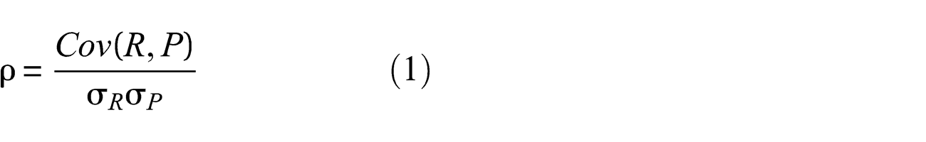
where the covariance, Cov, is

Cov (R, P) = \frac{\sum_{i}^{N} (R (t_{i}) - \bar{R}) (P (t_{i}) - \bar{P})}{N}

(2)

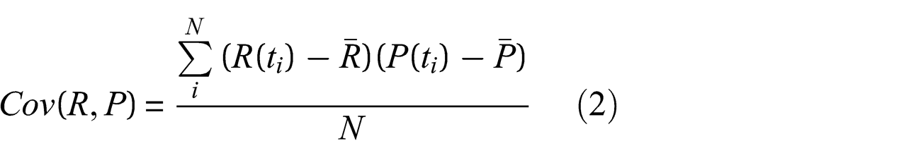
and the standard deviations, σ_R and σ_P, are

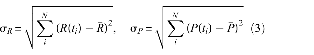
σ_{R} = \sqrt{\sum_{i}^{N} {(R (t_{i}) - \bar{R})}^{2}}, σ_{P} = \sqrt{\sum_{i}^{N} {(P (t_{i}) - \bar{P})}^{2}}

(3)

then, SDC = 1 − ρ.

It is evident that the degree of changes from a certain sensing path before and after damage is introduced will be clearly increased if the sensing path is close to the damage, and vice versa. Namely, SDCs for sensing paths closing to the damage are larger than those for paths away from the damage.

LSDC

Consider a spatially distributed array of N discrete sensors, each serve as both actuator and receiver. All of them are bonded to a plate under inspection at known locations. Due to reciprocity, there are a total of N(N − 1)/2 possible actuator–receiver pairs. Focusing on an arbitrarily selected pair for ith actuator and jth receiver as shown in Figure 1, let R_ij(t) denote the global received Lamb wave signal in the reference state and P_ij(t) denote the signal in the present state. Containing enough information, signals R_ij(t) and P_ij(t) can be regarded as functions of the structural properties of the whole monitored area in the reference and present states, respectively. However, local signals only containing structural property at a single point are needed here. 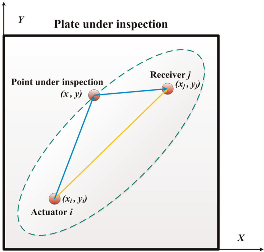Define that $R_{ij}^{xy} (t)$ and $P_{ij}^{xy} (t)$ represent such signals, exclusively related to the structural information at point (x, y). On the basis of R_ij(t) and P_ij(t), with assistance of the definition of ToF, $R_{ij}^{xy} (t)$ and $P_{ij}^{xy} (t)$ can be obtained.

Figure 1.

A graphical description of damage identification with a particular actuator–receiver pair.

ToF, which corresponds to the distance traveled by the wave,²¹ is one of the most straightforward and important features of a Lamb wave signal. Knowing the wave speed and the relative position among the actuator, receiver, and the point under inspection, we can calculate the ToF of the incident wave propagating from the actuator to the inspecting point and then to the receiver (the reflected wave is with the same mode as the incident one) as

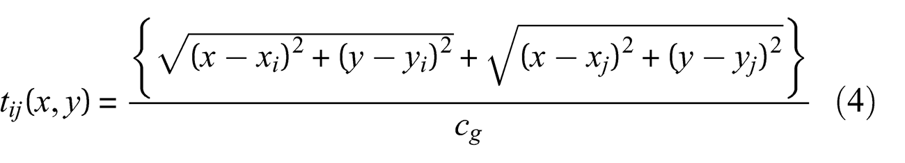
t_{ij} (x, y) = \frac{{\sqrt{{(x - x_{i})}^{2} + {(y - y_{i})}^{2}} + \sqrt{{(x - x_{j})}^{2} + {(y - y_{j})}^{2}}}}{c_{g}}

(4)

where (x, y), (x_i, y_i), and (x_j, y_j) denote the coordinates of the inspecting point, actuator, and receiver, respectively, and c_g is the group velocity of mode of interest. Lamb wave is multi-modal, which means the existence of at least two modes at any given frequency. In this article, only the wave mode with the maximum group velocity is considered. Applying a time-shift t_ij(x, y) and a windowing function to the global signals R_ij(t) and P_ij(t), respectively, we can get local signals $R_{ij}^{xy} (t)$ and $P_{ij}^{xy} (t)$ as

\begin{matrix} R_{ij}^{xy} (t) = R_{ij} (t + t_{ij}^{xy}) w (t) \\ P_{ij}^{xy} (t) = P_{ij} (t + t_{ij}^{xy}) w (t) \end{matrix}

(5)

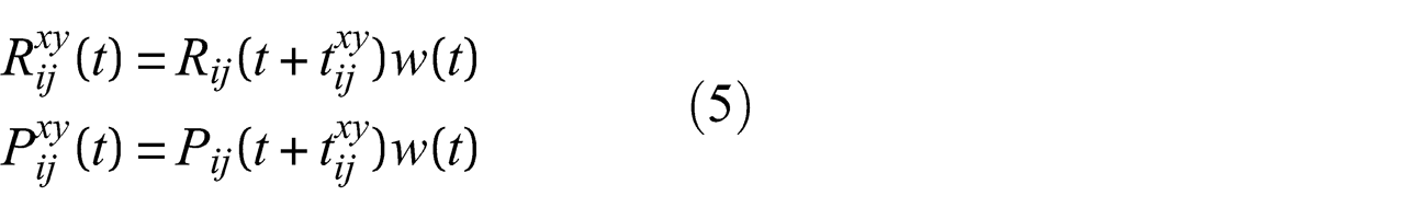
In equation (5), w(t) denotes a Hanning window centered at t = 0 with a given width. Here, window function can be employed to minimize the effects due to the structural property at positions other than (x, y).

Using a single sensor pair ij, the extracted local signals $P_{ij}^{xy} (t)$ and $R_{ij}^{xy} (t)$ are not linked with an exclusive point (x, y). All points on the ellipse whose foci are the two sensors, as shown in Figure 1, could yield the same t_ij(x, y), consequently generating the same local signals. Namely, $P_{ij}^{xy} (t)$ and $R_{ij}^{xy} (t)$ contain the information in structural integrity of all these points in the present and reference states, respectively. As the total N(N − 1)/2 sensor pairs are used, this issue could be mitigated, for the reason that the explicit point (x, y) is exclusively located via the intersection of multiple ellipses.

On substituting the extracted local signals $P_{ij}^{xy} (t)$ and $R_{ij}^{xy} (t)$ in equation (1) to solve for correlation coefficient ρ, we can get local signal difference coefficient, LSDC_ij(x, y) = 1 − ρ. Using the same method, LSDC at each point from every actuator–receiver pair can be calculated.

LSDC_ij(x, y) gives a value to describe structural variation at (x, y) in different states from a particular actuator–receiver pair ij. It is easy to understand that LSDC_ij(x, y) is 0 if no defect exists at (x, y). However, if a defect appears at (x, y), the corresponding local signal $P_{ij}^{xy} (t)$ is different from $R_{ij}^{xy} (t)$ due to the inclusion of damage-scattered wave component, LSDC_ij(x, y) is non-zero. Furthermore, the amplitude of the damage-scattered component is decreasing as the propagation distance increases, due to attenuation. As a result, the LSDC at damage location from a particular actuator–receiver pair will increase if the damage is close to the sensing path, and it will decrease if damage is far from the path.

Comparisons

Obviously, the major difference between LSDC and SDC is that the data used for calculation is different. Figure 2 schematically illustrates the calculation principles of the two features associated with ultrasonic signals, where R(t) denotes the reference signal and P(t) denotes the present signal, which are represented in the form of discrete sampling points. It is observed that SDC utilizes the global signals (global information), thus depicting the structural properties of the whole monitored area. Different from that, LSDC only utilizes a part of signal (local information); thus, it can describe structural status at each sole point within the monitoring area in detail. Both SDC and LSDC can indicate how close the damage location is from the sensing path. In addition, LSDC can also recognize the damage points, which helps to describe the structural information more accurately.

Figure 2.

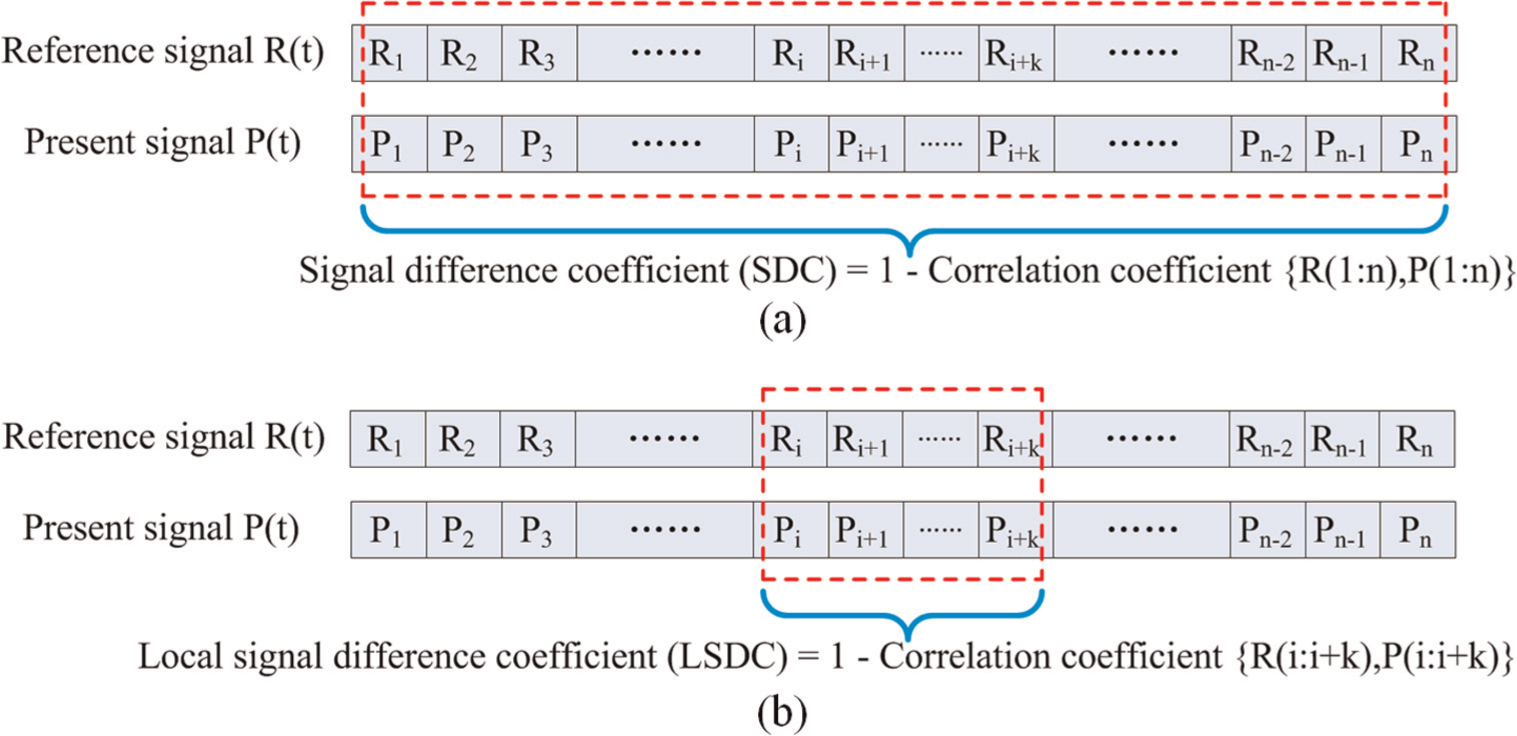
Calculation principles of tomographic features: (a) SDC and (b) LSDC.

Probability reconstruction algorithm based on LSDC

Probability reconstruction algorithm (PRA) describes a damage event using a visual image to indicate the probability of the presence of damage at a special point of the structure. In PRA, the damage area is always the image area where the probabilities are above a certain threshold. The grid with the highest value indicates the center of the identified damage. The formulation for the calculation is

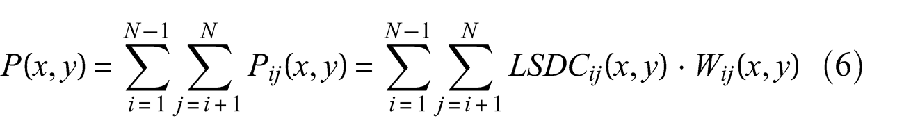
P (x, y) = \sum_{i = 1}^{N - 1} \sum_{j = i + 1}^{N} P_{ij} (x, y) = \sum_{i = 1}^{N - 1} \sum_{j = i + 1}^{N} LSD C_{ij} (x, y) \cdot W_{ij} (x, y)

(6)

where P(x, y) is the estimation of the defect probability at position (x, y) within the monitoring area and P_ij(x, y) is the estimation from the single actuator–receiver pair ij. N is the total sensors involved for damage identification. LSDC_ij(x, y) is the local signal difference coefficient at (x, y) from actuator–receiver pair ij, acting as the input feature for imaging. W_ij(x, y) is the weight given to the input feature. In a particular actuator–receiver pair, the weight acts as a linearly decreasing elliptical pattern where the two foci of the ellipse are the two sensor locations (Figure 3)

W_{ij} (x, y) = [\frac{β - R_{ij} (x, y)}{β - 1}]

(7)

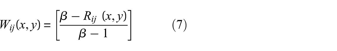
where

R_{ij} (x, y) = \frac{\sqrt{{(x - x_{i})}^{2} + {(y - y_{i})}^{2}} + \sqrt{{(x - x_{j})}^{2} + {(y - y_{j})}^{2}}}{\sqrt{{(x_{i} - x_{j})}^{2} + {(y_{i} - y_{j})}^{2}}}

(8)

Figure 3.

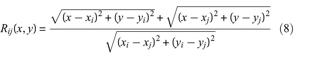
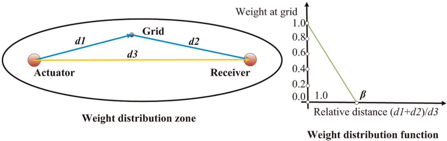
Illustration of the elliptical weight distribution of the PRA.

where (x, y) is the coordinate of the point under estimation; (x_i, y_i) and (x_j, y_j) are the coordinates of actuator i and receiver j, respectively. β is a scaling parameter which controls the size of the effective elliptical distribution area (i.e. controls the size of the affected zone of individual sensing paths) and the amplitude of which tapers from its maximum value along the line connecting the ellipse foci to zero on the periphery of the ellipse²²

W_{ij} (x, y) = {\begin{matrix} (β - R_{ij} (x, y)) / (β - 1) & when R_{ij} (x, y) < β \\ 0 & when R_{ij} (x, y) \geq β \end{matrix}

(9)

Given the weight function, the calculation of LSDC could be simplified. In fact, for a particular actuator–receiver pair, only the points within the affected zone of the sensing path are required for feature calculation, and that for external points are directly considered as zero, for the reason that the weights for these positions are equal to zero.

Performance analysis

Two imaging methods are employed for comparisons: (1) SDC-based PRA and (2) LSDC-based PRA. Localization accuracy and background noise level are compared for different algorithms.

Damage localization accuracy

In PRA, SDC and LSDC capture the global and local change of the ultrasonic signals, respectively. Any localized defects in the structure may lead to a special change in their values. Generally, if a defect occurs, signals from the transmitter–receiver pairs will be affected. For each pair, the calculated feature may be attributed to the defect distribution estimation of a sub-area of the reconstruction region. This sub-area is located in the ellipse where the corresponding actuator and receiver are foci (Figure 3(left)), and the probability estimation for this sub-area from the particular sensor pair is named as “hypothetical defect” here. As a result, the overall defect distribution probability can be calculated as a linear summation of all the “hypothetical defect” models from each possible actuator–receiver pair, and the point having the dominant probability would be regarded as the position where the defect is located. In this localization manner, it is easy to understand that the accuracy of the elliptical “hypothetical defect” model in depicting damage location from each actuator–receiver pair, in a certain degree, influences the final localization accuracy.

In SDC-based PRA, for a particular actuator–receiver pair, the “hypothetical defect” acts as a linearly decreasing ellipse from its maximum value along the line connecting the foci to zero on the periphery of the ellipse. The value distribution coincides with the weight distribution function as shown in Figure 3(right). Unfortunately, such an elliptical model cannot accurately indicate the actual damage position because wherever the damage locates, the peak falls along the direct path. To investigate the negative effect caused by this model, a damage identification case using a circular sensor array consisting of eight sensors is considered, as shown in Figure 4(a). It is observed that the sensing paths, Path 1, Path 2, and Path 3, are close to the damage; for this reason, the SDC values of them are larger than others. With larger features, these paths make more contributions for identifying the position of damage, which are called key paths. However, due to the characteristic of “hypothetical defect” model, an extremely high probability value may appear at the intersection of these three sensing paths rather than the actual damage location, which will yield an incorrect prediction of the position of damage.

Figure 4.

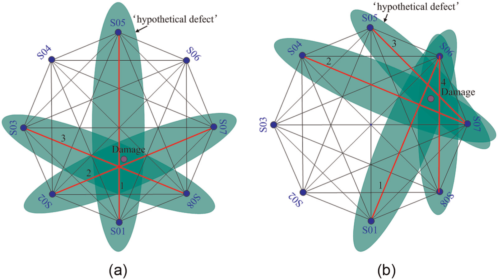
Probability-based damage identification via superposition of “hypothetical defect” models for every actuator–sensor pairs: (a) Case I and (b) Case II.

For another case in Figure 4(b), Path 1, Path 2, Path 3, and Path 4 are the key paths for the same reason. The peak probability (i.e. the maximum in the constructed probability image, which usually indicates the center of the damage) is preliminarily predicted to fall within the quadrilateral area consisting of these paths due to the superposition of their corresponding “hypothetical defect” models. However, an accurate estimation of the peak position is not available because the actual damage position cannot always be bigger than other non-damage points within each “hypothetical defect” model. Consequently, the peak probability may not appear at the actual damage position.

Based on previous analysis, it can be concluded that the inaccuracy of the “hypothetical defect” model for each actuator–receiver pair will cause localization error to some extent. In practice, the inaccuracy originates from the fact that the total points (i.e. damage points and intact points) within the affected zone share the same SDC. Different from that, if LSDC is employed as the input feature, each point has a corresponding LSDC. Furthermore, as mentioned in section “Tomographic feature,” damage points can be recognized with much larger LSDC. Therefore, in LSDC-based PRA, the “hypothetical defect” model has the maximum at the damage location and thus can indicate actual damage localization accurately. With superposition of accurate models, for Case I, the probability value at the intersection will be considerably decreased, while the actual damage position is highlighted; for Case II, similarly, compared with the intact points within the quadrilateral area, the actual damage position is also highlighted.

Background noise level

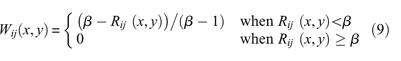
In PRA, it is easy to understand that the calculation result mainly depends on the paths close to the defect, and the far paths affect little. In particular, sensing paths corresponding to affected zones isolated from any localized defect have no influence on damage localization because the weights for damage position are equal to zero, based on equation (9). Generally, these paths are named as invalid sensing paths as shown in Figure 5. The superposition of the total “hypothetical defect” models of individual invalid paths constructs the background noise of the final image. At a particular point within the background area (e.g. sensor positions in Figure 4), which is provided with a large number of paths, as a result, the noise may be as large as the probability value at the actual damage position. In some cases, the noise is even larger, which will cause a wrong localization result. Therefore, with the goal of both reducing overall noise level and eliminating misleading information, the “hypothetical defect” model for invalid path should have a considerable low level in value.

Figure 5.

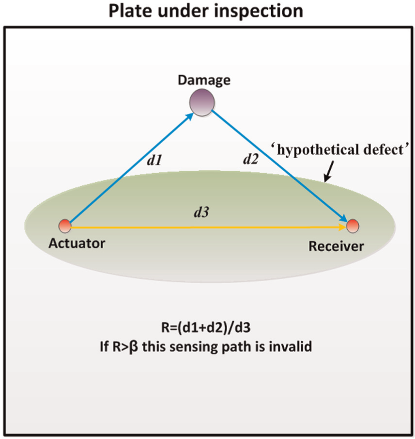
Definition of invalid sensing path.

For an arbitrarily selected invalid path as illustrated in Figure 5, the difference between present signal and reference signal comes from three components: (1) damage-scattered wave of each mode, (2) reflected wave from boundary after scattering by damage, and (3) mode conversion caused by damage. If the global signal is employed (i.e. SDC is employed), all the components above will be captured. However, LSDC does not have those components. In addition, the effects caused by interference at the beginning of the signal (e.g. electromagnetic interference^23,24) can be alleviated in LSDC. As a result, for any point within the affected zone, the corresponding local signals are identical between the reference and present states, which will result in that LSDCs at these points approach zero. With negligible input feature, the overall value of the “hypothetical defect” model is low, thus achieving the goal of reducing background noise.

Specimens and experimental setup

Experiments were carried out on four same aluminum plates (Specimens A, B, C, and D) with dimensions 500 × 500 × 2 mm³ to validate the improvement of the proposed LSDC-based PRA in imaging performance. Each plate was bonded with a circular sensor array consisting of eight piezoelectric ceramic disks with diameter of 8 mm and thickness of 0.5 mm. A photograph of the specimen with the active sensor network installed is illustrated in Figure 6. The monitoring area enclosed by the lead zirconium titanate (PZT) has the dimension of ∅252 mm. A coordinate system was employed with the plane of the monitoring area spanned by the horizontal, x, and vertical, y, axes, where the origin of coordinates was set to be the center of the circle. For Specimens A–C, a single artificial damage was introduced in the form of through-thickness hole with a diameter of ∅8.5 mm. For Specimen D, two same through-thickness holes (Damages I and II) are introduced. The coordinates of the center of the actual damage for Specimens A, B, and C were (−56.5, 24), (74, 9), and (59, −44), respectively. For Specimen D, the Damage I locates at (−16, 89) and Damage II locates at (−63, −63). Figure 7(a)–(d) illustrates the schematic diagrams of Specimens A–D with employed coordinate system and introduced damage, respectively.

Figure 6.

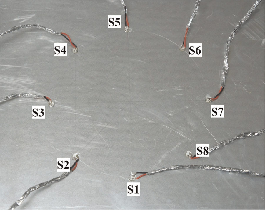
The specimen with a circular sensor array installed.

Figure 7.

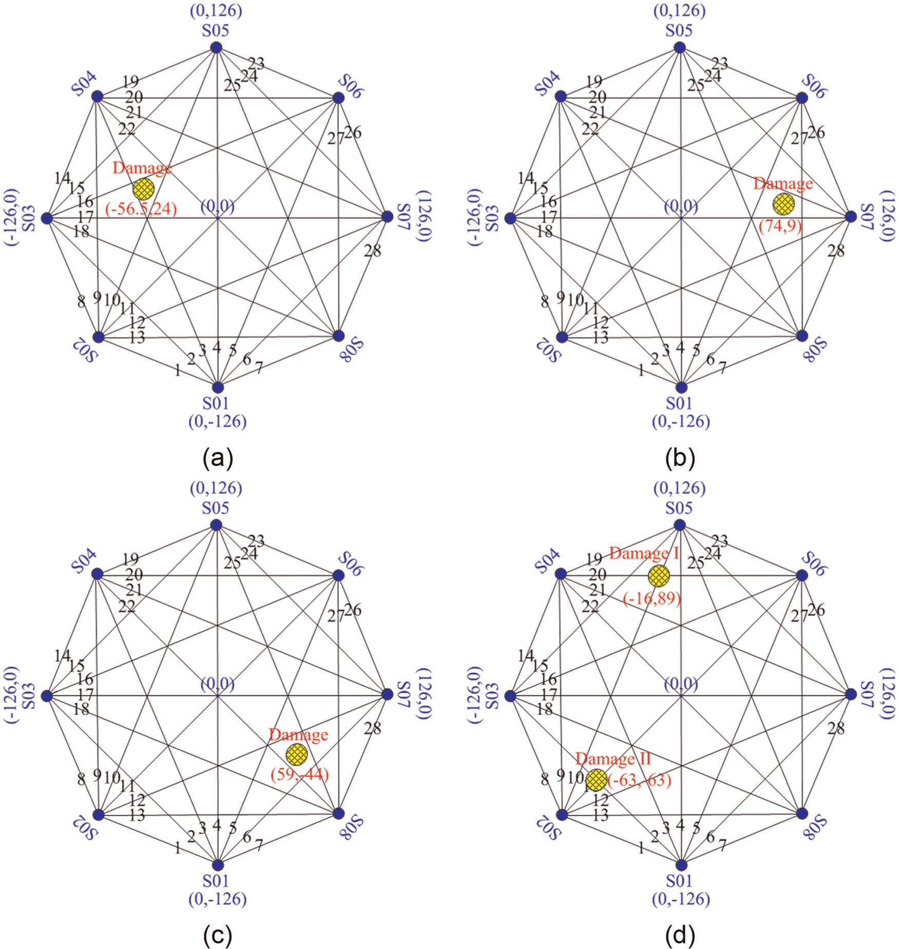
Specimens (a) A, (b) B, (c) C, and (d) D with employed coordinate system and introduced defect.

The experimental setup consists of an Agilent 33220A function/arbitrary waveform generator, a Piezo Systems EPA-104 voltage amplifier, two AVANT NI-2000 conditioning amplifiers, and a NI PXIe-1082 data acquisition. In this study, a 5-period Hanning-windowed sinusoidal tone burst signal centered at 150 kHz was generated as the input signal to drive the PZT actuator. In the active sensor network, the PZT elements take turns generating ultrasonic signals while the rest of them are listening. As shown in Figure 7, the current active sensor network provides 28 sensing paths in total. These sensing paths covered the inspected area within the circle. For each specimen, enough key paths locating in the vicinity of the damage could be employed to interrogate the presence of damage.

With the excitation signal centered at 150 kHz, only fundamental modes A0 and S0 propagate in the specimens. With a much higher group velocity, the S0 mode, rather than the A0 mode, was selected. The group velocity of S0 mode at 150 kHz is 5412.1 ms⁻¹. The window width in equation (5) was set as 33.3 µs, which coincides with the duration of the excitation/incident signal. Without considering the dispersion of S0 mode because it is weak and negligible, this data length helps to extract and contain the whole damage-reflected wave component.

Results analysis

Consider the experiment in Specimen A. The Lamb wave signals captured from different sensing paths (i.e. Paths 3, 9, and 13) are shown in Figure 8. The blue lines represent the signals in the reference state (without damage), while the red lines represent the signals in the present state (with damage). For each wave signal, after introduction of damage, localized wave component is changed, and the changed part is marked by dashed line rectangle for visibility. For further illustration, Figure 9(a) plots the LSDCs at damage point (i.e. (−56.5, 24)) for the total sensing paths. (Most LSDCs are directly set at zero due to the concept of invalid path, as mentioned in section “Background noise level.”) For comparison, LSDCs at non-damage point (e.g. the origin (0, 0)) are plotted in Figure 9(b), where a noticeable decrease in values is observed, implying high sensitivity of LSDC model in recognizing the structural status at a sole point.

Figure 8.

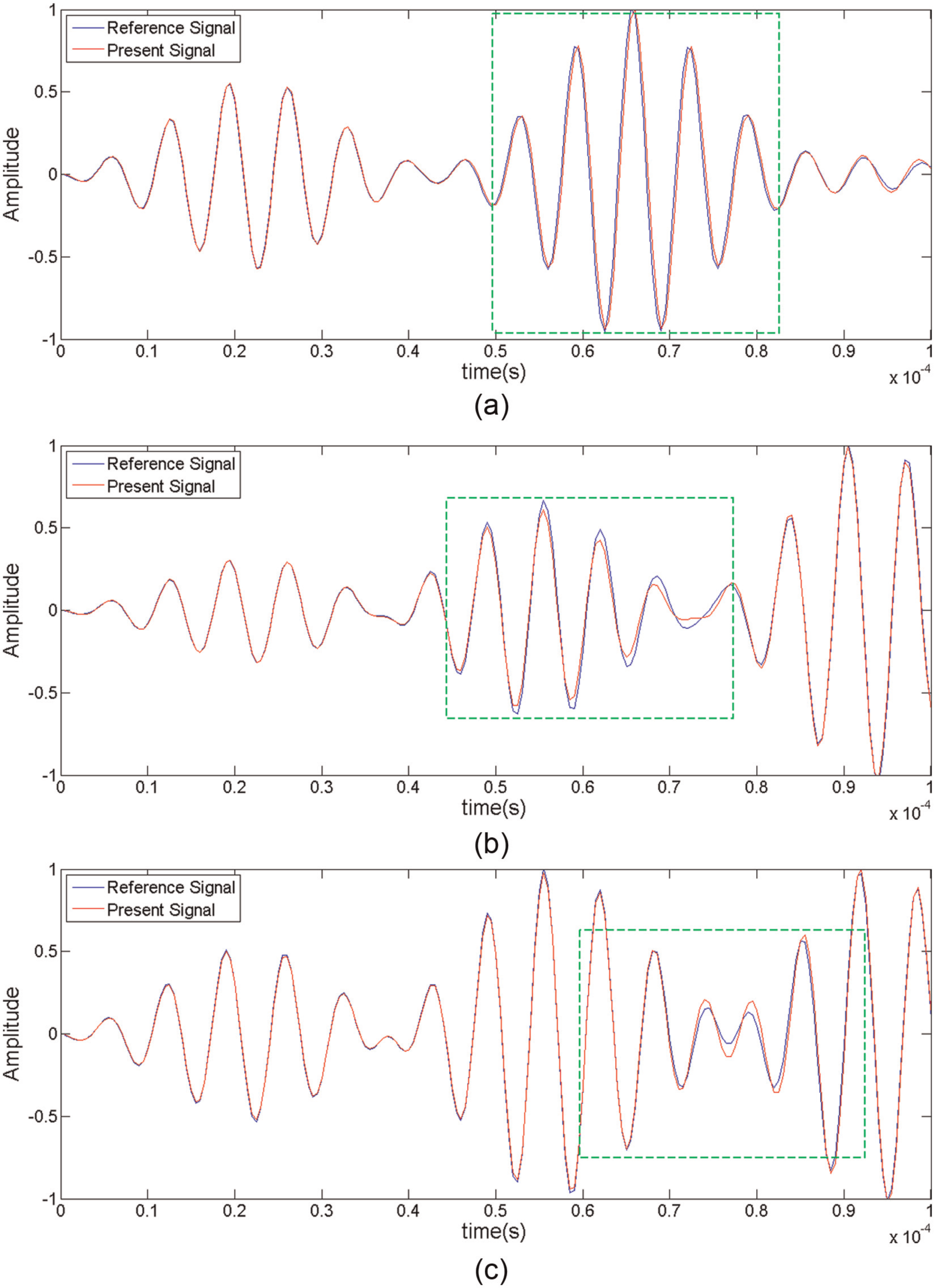
Lamb wave signals from different sensing paths: (a) Path 3, (b) Path 9 and (c) Path 13 in Specimen A.

Figure 9.

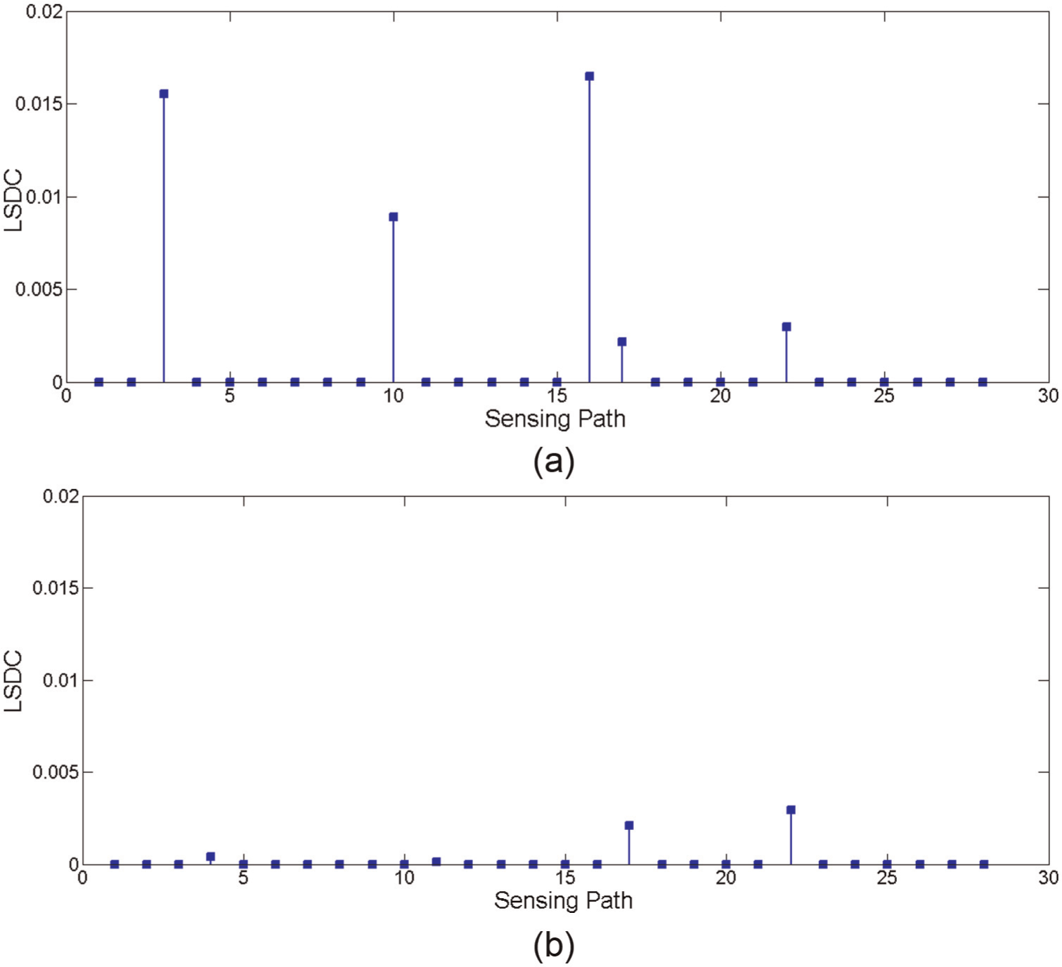
LSDCs for total sensing paths calculated using (a) the damage point (−56.5, 24) and (b) the origin (0, 0).

Figures of merit

Several figures of merit are defined to quantitatively evaluate the imaging performance, including both the localization accuracy and the background noise level. The localization error, simply the distance between the actual location of damage and the center of identified damage, is defined to evaluate the localization accuracy. To evaluate the background noise level, the reconstruction image is divided into two regions: (1) the damage region, where the probability values are above the specified threshold, which is set as 0.9 with the range of possible probability values normalized as 0–1, and (2) the background region, which is the remainder of the image (i.e. the damage region is excluded). It is noted that some vulnerable points (e.g. locations of sensors) are included in background region though they may have values above the threshold. The background noise can be quantified by two values: the peak and average of all the probability values falling in the background region. The average noise is able to depict noise level in respect of overall value. The peak noise is defined to describe the misleading information. For a reconstruction image, the peak is 0.9 if no vulnerable points show abnormal high values. However, the peak is above 0.9, and in some cases, it may even be 1, if the noise is strong enough to affect damage localization with the value above the given threshold.

Results with a specified scaling parameter

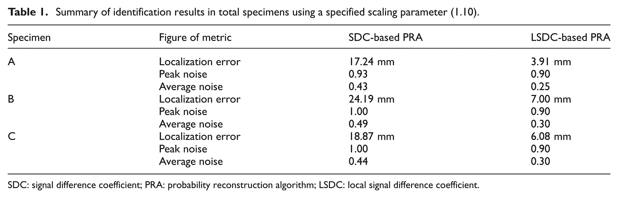
The scaling parameter, β, is first set as 1.10. Figure 10 illustrates the SDC- and LSDC-based probability images for Specimens A–C. The center location of the actual damage is marked by “+” and the identified damage (the grid with the highest probability value in the damage region) is marked by “o.” The images have the dimensions of 300 × 300 mm², that is, 300 × 300 uniformly distributed grids with an interspatial distance of 1 mm, being larger than the circular monitoring area. It is noteworthy that the probability values for the points outside the circle are not involved in the calculation of aforementioned figures of merit due to their insignificance in damage identification. With effective values used, the identification results in terms of localization accuracy and background noise level are summarized in Table 1.

Figure 10.

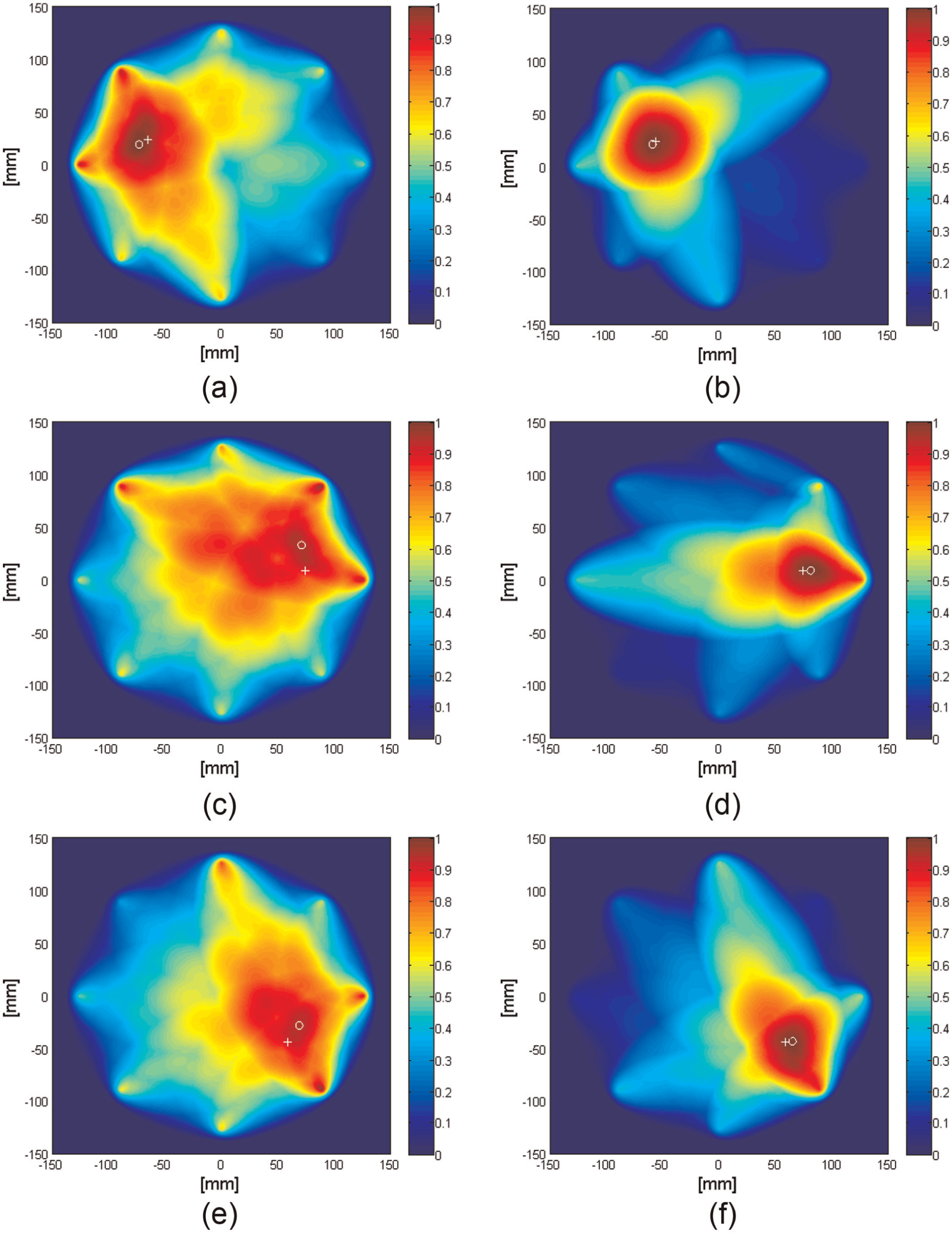
The probability images constructed using different input features for different specimens (β = 1.10): (a) SDC, Specimen A; (b) LSDC, Specimen A; (c) SDC, Specimen B; (d) LSDC, Specimen B; (e) SDC, Specimen C; and (f) LSDC, Specimen C.

Table 1.

Summary of identification results in total specimens using a specified scaling parameter (1.10).

Specimen	Figure of metric	SDC-based PRA	LSDC-based PRA
A	Localization error	17.24 mm	3.91 mm
	Peak noise	0.93	0.90
	Average noise	0.43	0.25
B	Localization error	24.19 mm	7.00 mm
	Peak noise	1.00	0.90
	Average noise	0.49	0.30
C	Localization error	18.87 mm	6.08 mm
	Peak noise	1.00	0.90
	Average noise	0.44	0.30

SDC: signal difference coefficient; PRA: probability reconstruction algorithm; LSDC: local signal difference coefficient.

Referring to Table 1, the images of Figure 10(a), (c), and (e) illustrate the typical characteristics of images generated from SDC-based PRA. First, the localization errors (17.24, 24.19, and 18.87 mm) are acceptable; the error is less than 25 mm even in the worst case, which shows that SDC-based PRA is reasonably effective in locating damage. Second, the background noise roughly decreases with an increment in relative distance of the point from the center of identified damage, and thus, the distribution has no negative effect on damage localization. However, at some vulnerable points (e.g. locations of Sensors 3, 6, and 8 for Specimens A, B, and C, respectively), abnormal phenomenon appears with values larger than given threshold, even larger than the probability value for the center of identified damage, as evidenced by a maximum background noise of 1.

With the employment of LSDC, the images of Figure 10(b), (d), and (f) clearly have improved imaging performance. In terms of localization accuracy, the localization errors are considerably reduced with all defects being unambiguously located very close to their actual positions. The largest localization error corresponding to identification in Specimen B is only 7.00 mm. In addition, the background noise statistics also shows considerable improvement with overall value (i.e. average noise) lowered from approximately 0.4–0.5 to 0.25–0.3. More importantly, the misleading information at vulnerable point is also eliminated, as indicated by peak noise of 0.9 in Table 1.

Results with different scaling parameters

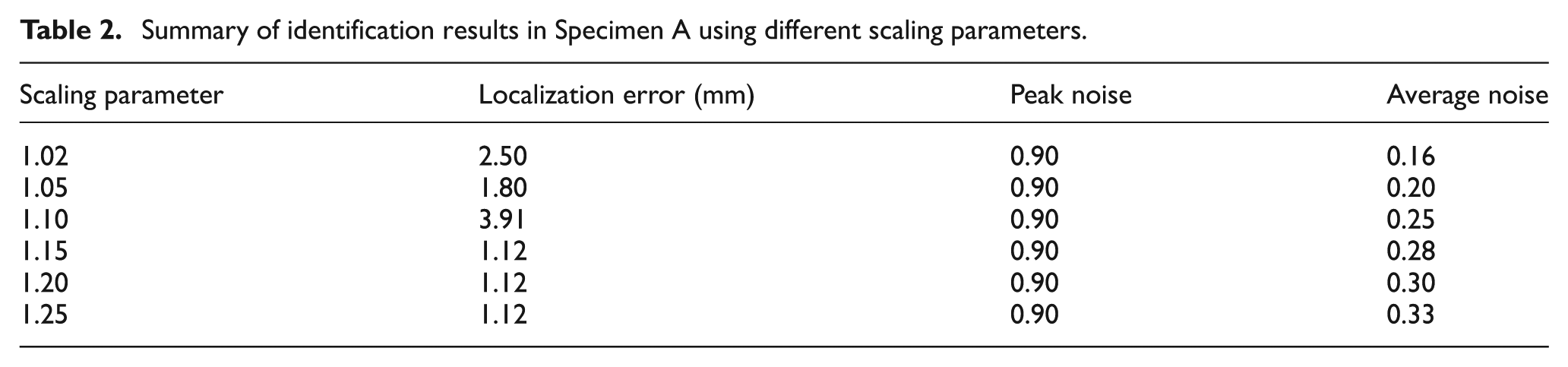
The results shown in Figure 10 and Table 1 indicate that the LSDC-based PRA is able to construct images with higher resolution at a specified scaling parameter (1.10). In practice, the scaling parameter β is selected empirically. β is taken 1.02, 1.05, 1.10, 1.15, 1.20, and 1.25, respectively, to investigate how it influences the damage identification result. Specimen A is employed for this investigation. Figure 11 illustrates the LSDC-based probability images constructed using these scaling parameters, and Table 2 lists the corresponding identification results.

Figure 11.

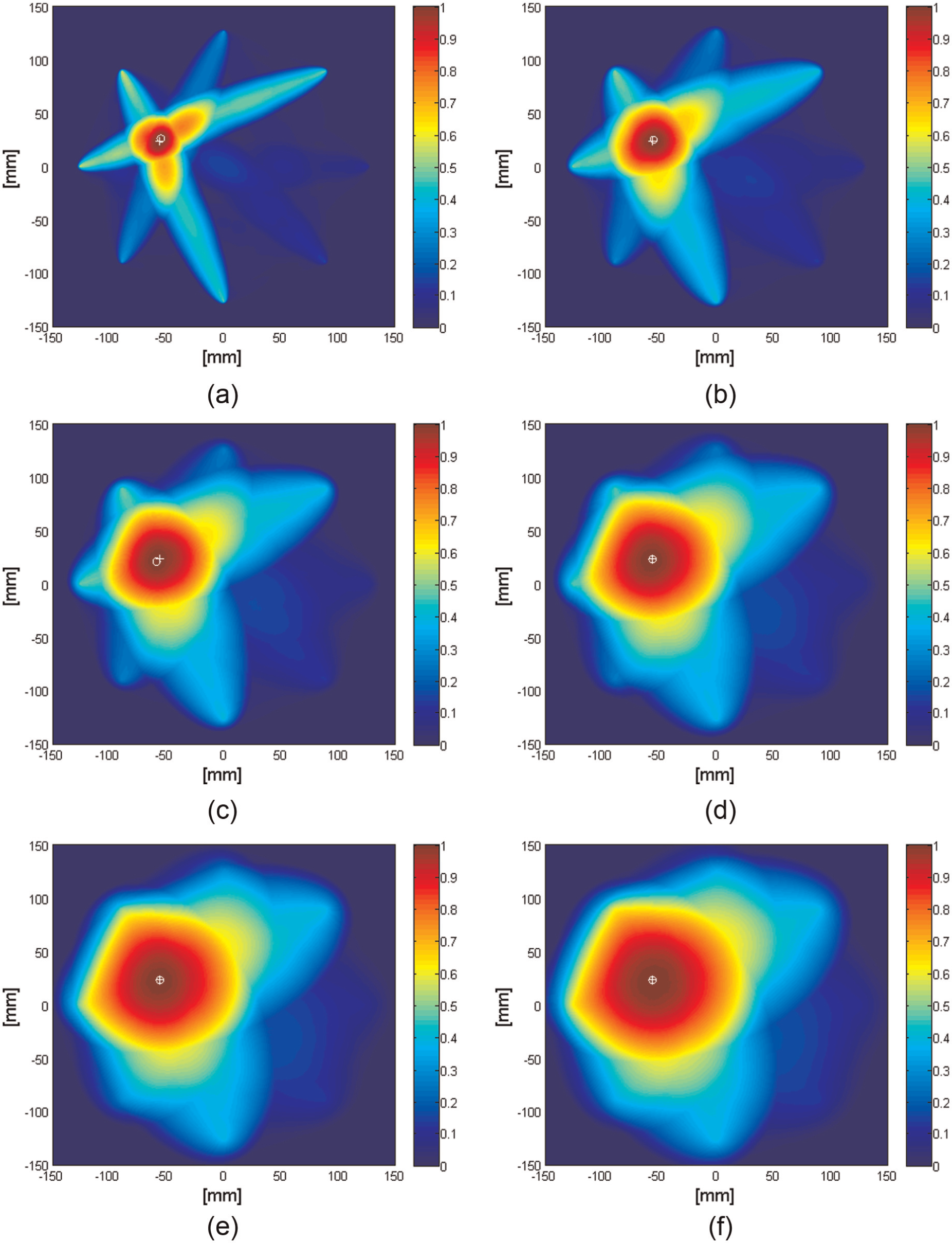
LSDC-based probability images in Specimen A constructed using different scaling parameters: (a) 1.02, (b) 1.05, (c) 1.10, (d) 1.15, (e) 1.20, and (f) 1.25.

Table 2.

Summary of identification results in Specimen A using different scaling parameters.

Scaling parameter	Localization error (mm)	Peak noise	Average noise
1.02	2.50	0.90	0.16
1.05	1.80	0.90	0.20
1.10	3.91	0.90	0.25
1.15	1.12	0.90	0.28
1.20	1.12	0.90	0.30
1.25	1.12	0.90	0.33

As shown in Figure 11, the total images have satisfactory localization accuracy. In practice, localization error changes only a little (1.12–3.91 mm) when the scaling parameter is selected in an appropriate range. Hence, it can be concluded that LSDC has the capability to provide improved localization accuracy at any scaling parameter within the appropriate range.

In terms of background noise, referring to Table 2, it is observed that the overall noise level increases with an increment in scaling parameter, symbolized from 0.16 to 0.33 when β varies from 1.02 to 1.25. The reason behind is that a large scaling parameter enlarges the affected zone of each sensing path. In practice, the image gives the largest noise level 0.33 when β = 1.25, and even this value is much less than that (0.43) in SDC-based algorithm when β = 1.10 (Figure 10(a)), which indicates the ability of the LSDC in lowering background noise at any scaling parameter. Furthermore, with all noise peaks equal to 0.90, the misleading information is also eliminated at any scaling parameter.

Results of multiple damage identification

By performing the aforementioned experiments in Specimens A–C, the high-resolution identification of single damage is achieved. Next, Specimen D is employed for multiple damage identification. The corresponding SDC- and LSDC-based probability images (β = 1.05) are shown in Figure 12(a) and (b), respectively. In Figure 12(a), it can be seen that the area around Damage I (the upper one) is much darker than that around Damage II (the lower one), indicating more severe damage, which, however, is contradictory to the fact that Damage I is the same as Damage II in size. The most probable reason for this confusing phenomenon is the intersection of key paths for the different instances of damage. In Figure 12(b), it is observed that the application of LSDC can relieve this problem.

Figure 12.

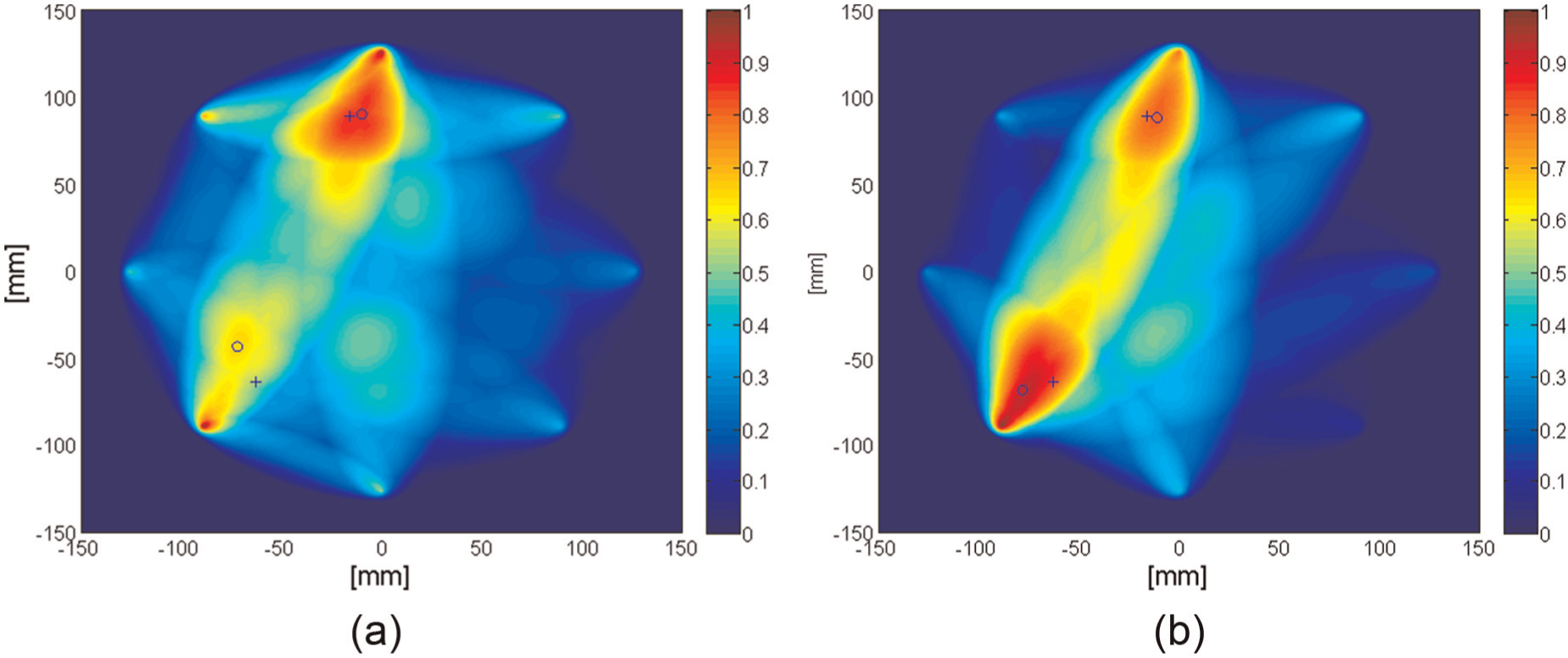
The probability images constructed using different input features in Specimen D: (a) SDC and (b) LSDC.

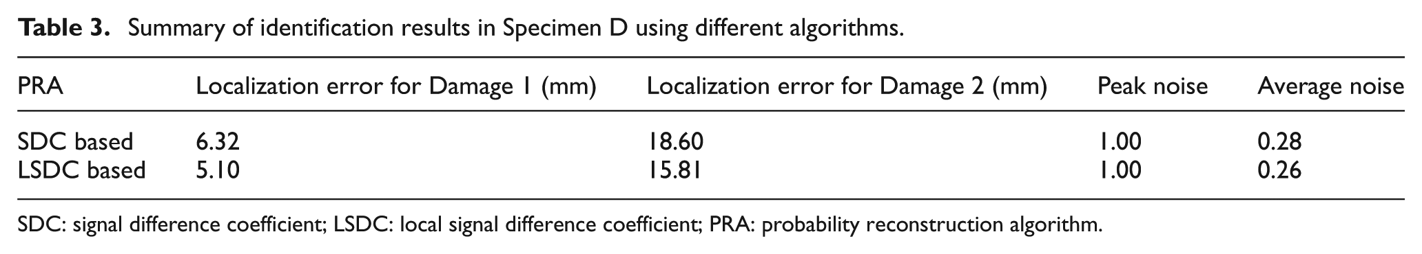
For clearer comparison, Table 3 lists the identification results. As can be seen, the LSDC-based image has lower localization errors for both Damage I and Damage II, and it also has lower overall noise level. However, with both noise peaks equal to 1.0, the misleading information at the locations of Sensor 2 and Sensor 5 is not eliminated, which is attributable to the fact that both Damage I and Damage II locate coincidentally close to the Path 10 (i.e. path Sensor 2–Sensor 5). In practice, this issue could be mitigated by advanced networks, where more key paths will be employed.

Table 3.

Summary of identification results in Specimen D using different algorithms.

PRA	Localization error for Damage 1 (mm)	Localization error for Damage 2 (mm)	Peak noise	Average noise
SDC based	6.32	18.60	1.00	0.28
LSDC based	5.10	15.81	1.00	0.26

SDC: signal difference coefficient; LSDC: local signal difference coefficient; PRA: probability reconstruction algorithm.

Discussion

In the proposed method, the imaging performance can be further improved by properly choosing the length of extracted local signal, which is performed by adjusting the window width in equation (5). In this article, the same length is used for all spatial points, and it is centered at the time calculated as equation (4). For the experiments in section “Results analysis,” the length is 33.3 µs.

We can obtain the optimal length for local signal through investigating the relationship between the length and the imaging performance. In Specimens A, B, and C, the localization accuracy is investigated with local signal length ranging from 3.3 to 39.6 µs with an increment of 3.3 µs (i.e. from 0.1 to 1.2 T in 0.1 T increments with T denoting the time duration of the excitation signal). The results are illustrated in Figure 13. It is observed that the localization error increases with inappropriate data length, both too short and too long.

Figure 13.

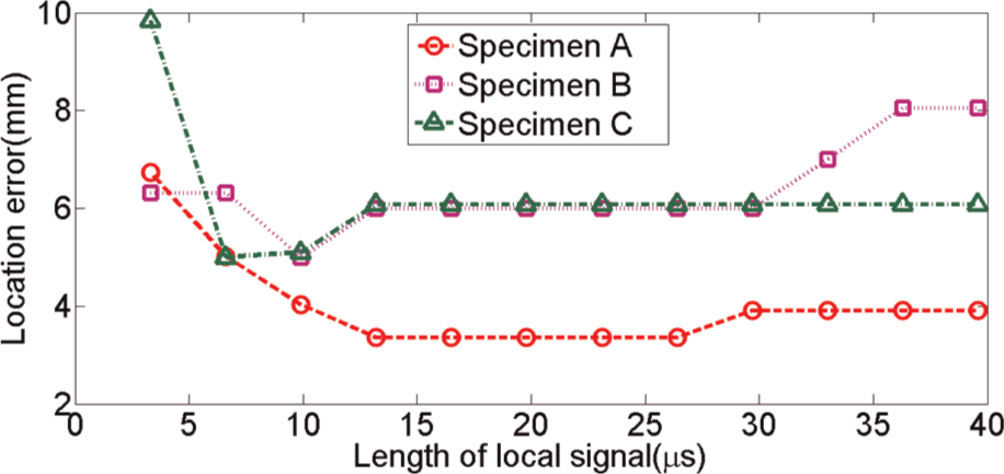
Localization error in Specimens A–C (β = 1.10) as the length of local signal changes from 3.3 to 39.6 µs with an increment of 3.3 µs.

In fact, the length of the local signal is determined to balance the need to (1) avoid magnification of weak/small signal difference independent of the presence of damage and (2) minimize the impact of undesired reflections. For an extremely short local signal, a fairly small disagreement between the signals may spoil the imaging performance completely. In contrast, for too long local signal, the opportunity of introduction of undesired reflection increases, which affects the capability of LSDC in recognizing damage, and thus influences the imaging performance. Considering both factors, several de-noising techniques (e.g. filter) could be employed previously to give signals with high SNR, after that, short local signal length will work effectively.

Conclusion

LSDC is a new tomographic feature that can be employed in PRA for damage identification. Compared with SDC, LSDC depicts damage information more accurately. Some conclusions can be obtained through the investigation in this article:

In LSDC-based PRA, the “hypothetical defect” model of individual path indicates the damage position accurately, which is not available in SDC-based algorithm. With superposition of effects from total paths, LSDC provides improvement in localization accuracy.

In LSDC-based PRA, the background noise constructed by invalid paths is lowered, for the reason that the influence on invalid paths from damage is excluded in employed local signal.

Footnotes

Funding

The work is supported by the National Natural Science Foundation of China (grant no. 51125022) and the Fundamental Research Funds for the Central Universities of China (grant no. CXTD2014001).

References

Rose

. Ultrasonic waves in solid media. New York: Cambridge University Press, 1999.

Malyarenko

Hinders

. Ultrasonic Lamb wave diffraction tomography. Ultrasonics 2001; 39(4): 269–281.

Leonard

Malyarenko

Hinders

. Ultrasonic Lamb wave tomography. Inverse Probl 2002; 18(6): 1795–1808.

Prasad

Balasubramaniam

Krishnamurthy

. Structural health monitoring of composite structures using Lamb wave tomography. Smart Mater Struct 2004; 13: N73–N79.

Nagata

Huang

Achenbach

. Lamb wave tomography using laser-based ultrasonics. Rev Prog Q 1995; 14: 561–568.

McKeon

JCP

Hinders

. Parallel projection and crosshole Lamb wave contact scanning tomography. J Acoust Soc Am 1999; 106(5): 2568–2577.

Malyarenko

Hinders

. Fan beam and double crosshole Lamb wave tomography for mapping flaws in aging aircraft structures. J Acoust Soc Am 2000; 108(4): 1631–1639.

Leonard

Hinders

. Lamb wave tomography of pipe-like structures. Ultrasonics 2005; 43(7): 574–583.

Belanger

Cawley

. Lamb wave tomography to evaluate the maximum depth of corrosion patches. Rev Quant Nondestruct Eval 2008; 27: 1290–1297.

10.

Belanger

Cawley

. Feasibility of low frequency straight-ray guided wave tomography. NDT&E Int 2009; 42(2): 113–119.

11.

Zhao

Royer

Owens

. Ultrasonic Lamb wave tomography in structural health monitoring. Smart Mater Struct 2011; 20: 105002.

12.

Gao

Shi

Rose

. Guided wave tomography on an aircraft wing with leave in place sensors. Rev Quant Nondestruct Eval 2005; 24: 1788–1794.

13.

Hay

Royer

Gao

. A comparison of embedded sensor Lamb wave ultrasonic tomography approaches for material loss detection. Smart Mater Struct 2006; 15(4): 946–951.

14.

Koduru

Rose

. Guided wave annular array sensor design for improved tomographic imaging. Rev Quant Nondestruct Eval 2009; 28: 658–665.

15.

Wang

. Probability of the presence of damage estimated from an active sensor network in a composite panel of multiple stiffeners. Compos Sci Technol 2009; 69(13): 2054–2063.

16.

Wang

. A damage diagnostic imaging algorithm based on the quantitative comparison of Lamb wave signals. Smart Mater Struct 2010; 19(6): 065008.

17.

Zhao

Gao

Zhang

. Active health monitoring of an aircraft wing with embedded piezoelectric sensor/actuator network: I. Defect detection, localization and growth monitoring. Smart Mater Struct 2007; 16(4): 1208–1217.

18.

Wang

. Time-domain analyses and correlations of Lamb wave signals for damage detection in a composite panel of multiple stiffeners. J Compos Mater 2009; 43(26): 3211–3230.

19.

Wang

. Probabilistic damage identification based on correlation analysis using guided wave signals in aluminum plates. Struct Health Monit 2010; 9(2): 133–144.

20.

Wang

. A probabilistic diagnostic algorithm for identification of multiple notches using digital damage fingerprints (DDFs). J Intel Mat Syst Str 2009; 20(12): 1439–1450.

21.

Tua

Quek

Wang

. Detection of cracks in plates using piezo-actuated Lamb waves. Smart Mater Struct 2004; 13: 643–660.

22.

Sheen

Cho

. A study on quantitative Lamb wave tomogram via modified RAPID algorithm with shape factor optimization. Int J Precis Eng Man 2012; 13(5): 671–677.

23.

Giurgiutiu

. Lamb wave generation with piezoelectric wafer active sensors for structural health monitoring. In: Proceedings of SPIE Smart Structures and Materials, San Diego, CA, 2 March 2003, vol. 5056, pp. 111–122. Bellingham, WA: SPIE.

24.

Giurgiutiu

. Tuned Lamb wave excitation and detection with piezoelectric wafer active sensors for structural health monitoring. J Intel Mat Syst Str 2005; 16(4): 291–305.